Article

Language-Based Opacity Verification in Partially Observed Petri Nets through Linear Constraints

1
Institute of Systems Engineering, Macau University of Science and Technology, Taipa, Macau SAR 999078, China
2
Mediterranean Institute of Technology, South Mediterranean University, Tunis 99628, Tunisia
3
Industrial Engineering Department, College of Engineering, King Saud University, P.O. Box 800, Riyadh 11421, Saudi Arabia
4
Hitachi Building Technology (Guangzhou) Co., Ltd., Guangzhou 510700, China
*
Author to whom correspondence should be addressed.
These authorscontributed equally to this work.
Mathematics 2023, 11(18), 3880; https://doi.org/10.3390/math11183880
Submission received: 7 August 2023 / Revised: 31 August 2023 / Accepted: 8 September 2023 / Published: 11 September 2023
(This article belongs to the Special Issue Dynamical Systems and System Analysis)

Abstract

:
Information security is an important area of concern in modern computer-integrated systems. It involves implementing preventative measures to protect confidential data from potential vulnerabilities, such as unauthorized access, secret disclosure, modification, or destruction. Considering such threats, we investigate a particular confidentiality property called opacity, which specifies a system’s ability to cover its ‘secret’ data from being interfered with by outside observers, termed as intruders. This paper discusses language-based opacity formulation and verification in the context of discrete event systems represented by partially observed Petri nets. In this context, we identify two opacity properties, called consistency and non-secrecy; then, we exploit the mathematical characterization of a net system, to separately check each property, by specifying two feasibility problems. The proposed method is carried out for two distinct settings of a system. The first setting is centralized, where an intruder is granted complete information about the system structure but a partial observation of its behavior. The second setting is decentralized, where a group of intruders cooperates to reveal the secret language, by using a coordinator. Finally, experimental findings are given, to demonstrate the proficiency of the proposed approach.

1. Introduction

The growing number of modern cyber-physical systems involving critical information, such as defense, health care, banking, and communication systems, emphasizes the need to establish measures to ensure their security against hostile actions. These systems are particularly subject to unauthorized access, because the risk of information leakage to unauthorized users may reveal sensitive details about their behavior.
Both the industry and the research communities have recently stressed the importance of security properties. These properties are primarily categorized into three groups: confidentiality, availability, and integrity, which guide policies for information security within systems and organizations. Motivated by security concerns about discrete event systems (DESs), our study concentrates on a specific confidentiality property, called opacity. This property describes the capability of preventing a hostile observer, referred to as an intruder, from inferring whether or not a system’s secret behavior has occurred. Numerous aspects of opacity have recently been investigated in the computer security community.
Due to their competency for system modeling, Petri nets under partial observations have been widely used in cyber-physical systems. In the area of DESs, there has been a deluge of studies on fault diagnosis, deadlock control [1], and supervisory control [2] based on Petri nets. One significant feature of a Petri net (PN) is its mathematical formalism that allows the use of integer linear programming (ILP), which can alleviate the state explosion problem, to some extent. For this reason, we use a Petri net as a modeling framework in this study.
Opacity is considered as a general information flow property that covers a wide range of applications in DESs. Bryans et al. [3] proved that certain information flow properties, such as anonymity and non-interference [4] problems, can be converted into opacity, by using appropriate observation mappings. In addition, Lin et al. [5] showed that observability, detectability, and diagnosability [6] can be conceived as opacity problems.
Opacity in DESs is categorized into two main groups, based on the secret’s representation: state-based opacity [7], where a secret is specified as a subset of the state space, and language-based opacity (LBO) [8], where a secret is specified as a subset of firable transition sequences.
This study considers the language-based opacity verification problem in DESs represented by partially observed Petri nets (POPNs), where a secret is defined as a finite sub-language of a PN system, and an intruder is allowed to possess complete knowledge of the system’s structure, but can only identify the firing of visible transitions and (or) the tokens variation in visible places. Language-based opacity was initially introduced to DESs modeled with FSA in [5,9], and it was extended recently to bounded labeled Petri net systems (LPNs) in [10]. In [5], Lin et al. specified two classes of opacity, called strong and weak opacity. A strongly (resp. weakly) opaque language is a language where strings from a different language camouflage all (resp. some) of its strings. Specifically, given a regular system language and a state-based projection information mapping, the authors in [5] proposed algorithms with exponential complexity, to verify both weak and strong opacity. In the current study, language-based opacity is attributed to strong opacity. In [10], Tong et al. studied a special case of LBO, called strict language opacity, in a bounded PN system. This work was based on the assumption that a secret is defined as a subset of firable sequences of transitions and an intruder who is interested in observable transitions only. To check the strict language opacity property, Tong et al. built a finite automaton, called a verifier, which synchronized the PN system and the secret language, based on observable transitions. This approach was time-consuming, because it required off-line construction of the verifier, which suffered an exponential space complexity. In [11], Cong et al. also established a necessary and sufficient condition for current state opacity (CSO) verification in LPN through integer linear programming. However, their method cannot be directly used for LBO verification, unless we convert the CSO problem into an LBO problem, using the transformation method given in [12]. Furthermore, the research in [11] only considered secret markings defined by a set of generalized mutual exclusion constraints (GMECs), which restricts the scope of secret selection.
Another interesting work is found in [13], which investigated the verification problem of LBO in LPNs, where the unobservable subnet was considered to be acyclic, and the secret was specified across sequences of events rather than transitions. The study in [13] was closely related to this particular research, in which the authors solved an integer linear programming problem (ILPP), to establish a condition that was both sufficient and necessary for LBO verification. The technique proposed in this study is more general, as it applies to a greater range of PN systems under partial observations (i.e., PNs equipped with place and transition sensors).
Nowadays, intruders tend to be highly skilled and intelligent. They are often part of an organized group providing illegal specialized services, such as credit card fraud, theft of intellectual property, or counterfeiting documents. This paper investigates the LBO verification problem in a decentralized setting, where local intruders collaborate by using a coordinator. Each local intruder has complete information about the net structure but only partial information about its evolution.
Decentralized opacity can be reduced to many security properties, such as decentralized anonymity, secrecy, and non-interference. Specifically, consider a multi-user system that allows many users to share the resources of a single computer. In our framework, these users can be viewed as intruders who should not determine whether or not the decentralized security property is met. Furthermore, many properties employed in discrete event systems for supervisory control can be restated as a particular instance of decentralized opacity. Paoli et al. [14] showed that co-opacity is an extension of co-observability [15] used for supervisory control [16], and that it can be used to check the existence of a group of decentralized local supervisors (intruders in our framework, with or without a coordinator) that control a system. Tripakis and Rudie [17] developed a decidable condition called “at least one can tell”, which ensures that decentralized agents can make correct decisions about the behavior of a system. This condition is relevant to the decentralized opacity problem, because it provides a way to verify whether or not a decentralized system is opaque.
This research aims to compose the LBO verification problem in the context of a DES represented by a POPN, taking into account observations from place and transition sensors. Then, based on the proposed formulation, new approaches to verifying LBO are set up. In light of the preceding, the findings of this study contribute the following to the existing literature:
  • We define the concept of secret observation sequences, by considering a case where a secret involves numerous transition sequences yielding the same observation. This concept decreases the effort required to check language opacity in a POPN, by avoiding redundant explorations.
  • We identify two language-based opacity properties, called consistency and non-secrecy properties; we separately check each property; then, we provide necessary and sufficient conditions to check language-based opacity, by defining and solving an ILPP.
  • Finally, we extend the above results from a centralized framework to a decentralized framework with a coordinator, where more than one intruder observes the system.
The following is a breakdown of the paper’s structure. Section 2 provides an overview of Petri nets and partially observed Petri nets. The theory underlying the partition of unobservable transitions, as well as the concept of discernible transitions, is presented in Section 3. The LBO verification problem is formulated in a POPN system in Section 4. An ILP problem is established in Section 5, to solve the LBO verification problem. In Section 7, we discuss opacity in a decentralized case, where a group of local intruders unites to reveal a secret language via a coordinator. To demonstrate the proposed method, an example is given in Section 6. Finally, Section 8 brings the study to a close and points the way forward for further research.

2. Preliminaries

2.1. Petri Nets

A Petri net structure is a weighted bipartite graph N = ( P , T , P r e , P o s t ) , where P = { p 1 , p 2 , , p m } is a set of m places and T = { t 1 , t 2 , , t n } is a set of n transitions with P T and P T = . P r e : P × T N and P o s t : P × T N ( N denotes the set of non-negative integer numbers) are the pre- and post-incidence functions designating arcs from places to transitions and from transitions to places, respectively, in a net, and they are represented as matrices in N m × n . The incidence matrix of a PN is defined by C = P o s t P r e .
A marking is a mapping M : P N that attributes to each place a non-negative integer number of tokens. A PN system with initial marking M 0 is denoted by a couple ( N , M 0 ) . A transition t i is enabled at a marking M, denoted by M [ t i , if M P r e ( · , i ) , where P r e ( · , i ) is the ith column of matrix P r e . Firing an enabled transition yields a marking M with
M = M + C ( · , t ) ,
where C ( · , t ) is a column vector that denotes the token change generated by firing t. Given a transition sequence σ T * , | σ | denotes the length of σ . Let π : T * N n be a function that allocates a Parikh vector y N n to a transition sequence σ T * , called the firing vector of σ . The notations M [ σ and M [ σ M indicate, respectively, that σ is enabled at M and the firing of σ at M yields M , following the equation:
M = M + C · π ( σ ) .
Equation (2) is called the state equation of ( N , M 0 ) . We denote by L ( N , M 0 ) = { σ T * | M 0 [ σ } the set of all firable transition sequences in ( N , M 0 ) , and by R ( N , M 0 ) the reachability set of ( N , M 0 ) . A PN is said to be acyclic if there is no directed circuit and bounded if there exists a positive constant k N , such that, for all M R ( N , M 0 ) and p P , M ( p ) k , where M ( p ) is the tokens number in place p.

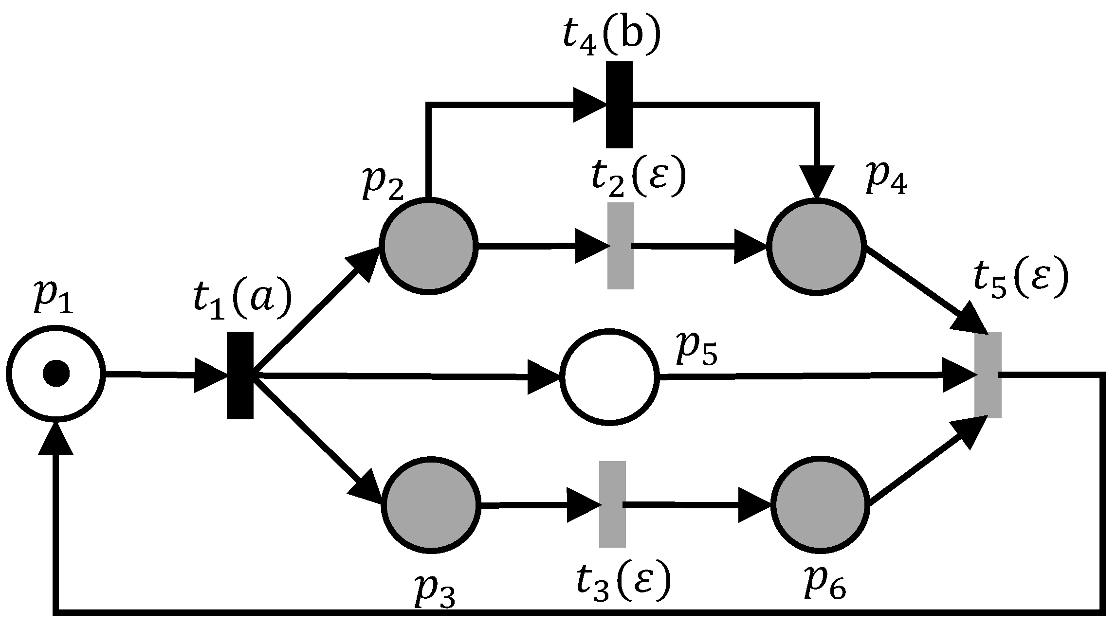
2.2. Partially Observed Petri Nets

A partially observed Petri net is a PN system equipped with place sensors that display the number of tokens in some places, known as observable places, and (or) transition sensors that display the labels of observable transitions, when fired. In this sense, POPNs can be seen as a generalization of LPNs, since any LPN can be represented as a POPN. However, not all POPNs can be represented as LPNs. This is because POPNs allow for the presence of place sensors, which LPNs do not.
The set of observable places is denoted by P o P . We re-index observable places in P o from 1 to m o , such that P o = { p o 1 , p o 2 , , p o m o } with o i { 1 , 2 , , m } and p o i P for i { 1 , 2 , , m o } . A partially observed Petri net is a quintuple-tuple Q = ( N , M 0 , E , V , δ ) , where ( N , M 0 ) is a PN system with m places and n transitions, E is an alphabet (a set of labels), and V = ( v i j ) { 0 , 1 } m o × m is a place sensor configuration matrix, where v i j = 1 if j = o i and v i j = 0 , otherwise. A labeling function, δ : T E { ε } , represents the transition sensor configuration, which allocates a label from E or the empty string ε to a transition t T . Based on these allocations, we divide the set of transitions T into two disjoint sets T o and T u , satisfying T = T o T u and T o T u = , where T o = { t T | δ ( t ) E } is the set of observable transitions and T u = { t T | δ ( t ) = ε } is the set of unobservable transitions. Thus, a label δ ( t ) is displayed only when we fire a transition t T o . We denote by M ^ = V · M the marking measurement of M using a place sensor configuration matrix V. Arguably, matrix V characterizes a marking M projection on P o .
Definition 1. 
Let ( N , M 0 ) be a PN system with N = ( P , T , P r e , P o s t ) . An evolution of N starting from M 0 is denoted as a transition-marking sequence.
M 0 t 1 M 1 t 2 M 2 t h M h ,
satisfying M 0 [ t 1 M 1 [ t 2 M 2 [ t h M h , where t i T , M i R ( N , M 0 ) for i { 1 , , h } , h 1 .
Definition 2. 
Given a POPN Q = ( N , M 0 , E , V , δ ) , the collected measure associated with M [ t M is given as follows:
ρ ( M , t ) = ε p , if ( M ^ = M ^ ) ( δ ( t ) = ε ) M ^ δ ( t ) M ^ , otherwise ,
where M ^ = V · M , M ^ = V · M and ε p denotes an empty observation.
We denote by ρ ( M , σ ) the extension of the operation ρ to transition sequences. Specifically, let M t 1 M 1 t 2 M 2 M h 1 t h M h be the evolution produced by firing σ = t 1 t 2 t h T * at M. We define the associated measurement sequence by concatenating the successive collected measures, as seen below:
ρ ( M , σ ) = ρ ( M , t 1 ) ρ ( M 1 , t 2 ) ρ ( M h 1 , t h ) = M ^ e 1 M ^ 1 M ^ 1 e 2 M ^ h o 1 M ^ h o 1 e h o M ^ h o ,
where e i E { ε } and h o h . Given a measurement sequence M ^ 0 e 1 M ^ i M ^ i e h o M ^ h o , 1 i h o 1 , the operation Λ fuses each two adjacent M ^ i as follows:
Λ ( M ^ 0 e 1 M ^ i M ^ i e h o M ^ h o ) = M ^ 0 e 1 M ^ i e h o M ^ h o .
Definition 3. 
Let Q = ( N , M 0 , E , V , δ ) be a POPN, M be a marking from R ( N , M 0 ) , and σ = t 1 t 2 t h T * be a transition sequence, such that M [ σ . The observation sequence generated when σ fires at M is
w ( M , σ ) = Λ ( ρ ( M , σ ) ) = Λ ( M ^ e 1 M ^ 1 M ^ 1 e 2 M ^ h o 1 M ^ h o 1 e h o M ^ h o ) = M ^ e 1 M ^ 1 e 2 M ^ h o 1 e h o M ^ h o .
Marking measurements are displayed by sensors whenever observable events fire or when token variations occur in observable places. After obtaining ρ ( M , σ ) , each two adjacent measures M ^ i M ^ i are merged into one measure, using the operation Λ . For simplification purposes, if no confusion is caused, we use the symbol w to designate an observation sequence in a POPN.
Example 1. 
Consider a POPN in Figure 1 with M 0 = [ 1 0 0 0 0 0 ] T . The place sensor configuration is derived from P o = { p 1 , p 5 } as follows:
V = p o 2 p o 1 p 1 p 2 p 3 p 4 p 5 p 6 1 0 0 0 0 0 0 0 0 0 1 0 .
We have T o = { t 1 , t 4 } and T u = { t 2 , t 3 , t 5 } . Given E = { a , b } , we define the event sensor configuration using the labeling function δ as δ ( t 1 ) = a , δ ( t 4 ) = b , and δ ( t 2 ) = δ ( t 3 ) = δ ( t 5 ) = ε . Let σ = t 1 t 3 t 4 be a transition sequence that is enabled at M 0 . By Definition 1, [ 1 0 0 0 0 0 ] T t 1 [ 0 1 1 0 1 0 ] T t 3 [ 0 1 0 0 1 1 ] T t 4 [ 0 0 0 1 1 1 ] T is the evolution generated by firing σ at M 0 . We have ρ ( [ 0 1 1 0 1 0 ] T , t 3 ) = ε p ; by Definition 3, the associated observation sequence is Λ ( ρ ( M 0 , σ ) ) = [ 1 0 ] T a [ 0 1 ] T b [ 0 1 ] T .
Let Q = ( N , M 0 , E , V , δ ) be a POPN and M be a marking from R ( N , M 0 ) . We define by
O ( Q , M ) = { w | σ T * , M [ σ , Λ ( ρ ( M , σ ) ) = w }
the set of feasible observation sequences generated by Q from M, and by
S ( w ) = { σ T * | M 0 [ σ , Λ ( ρ ( M 0 , σ ) ) = w }
the set of transition sequences consistent with w.

3. Quasi-Unobservable and Discernible Transitions

Let Q be a POPN with a sensor configuration ( V , δ ) and C o N m o × n be the restriction of C to P o . Based on C o , the set of unobservable transitions T u can be partitioned into two disjoint sets T ˜ q and T ˜ u , such that T u = T ˜ q T ˜ u and T ˜ q T ˜ u = , where T ˜ q = { t T u | C o ( · , t ) 0 m o ( 0 m o is an m o -dimensional column vector with all entries being 0)} is a set of quasi-observable transitions and T ˜ u = { t T u | C o ( · , t ) = 0 m o } is a set of truly unobservable transitions. We define T d = T o T ˜ q as the set of discernible transitions. For e E { ε } , T ( e ) = { t T | δ ( t ) = e } and T d ( e ) = { t T d | δ ( t ) = e } , respectively, represent the subsets of transitions in T and T d , having the same label, e. We denote by Γ e = { v t | v t = C o ( · , t ) , t T ( e ) } the set of column vectors in matrix C o associated with transitions in T ( e ) .
Example 2. 
Consider the POPN with the sensor configuration ( V , δ ) specified in Example 1. Matrix C o is given as follows:
C o = p 5 p 1 t 1 ( a ) t 2 ( ε ) t 3 ( ε ) t 4 ( b ) t 5 ( ε ) 1 0 0 0 1 0 0 0 0 1 .
It is evident that T ˜ u = { t 2 , t 3 } , T ˜ q = { t 5 } , and T d = { t 1 , t 4 , t 5 } .
Definition 4. 
Let Q = ( N , M 0 , E , V , δ ) be a POPN and T ˜ u be the set of its truly unobservable transitions. A truly unobservable subnet of Q is defined as Q ˜ = ( N ˜ , E , M 0 , V , δ ) , where N ˜ = ( P , T ˜ u , P r e ˜ u , P o s t ˜ u ) , with P r e ˜ u and P o s t ˜ u being, respectively, the restrictions of P r e and P o s t on T ˜ u . A discernible subnet of Q is defined as Q d = ( N d , M 0 , E , V , δ ) , where N d = ( P , T d , P r e d , P o s t d ) , with P r e d and P o s t d being, respectively, the restrictions of P r e and P o s t on T d . C ˜ u and C d , respectively, denote the incidence matrices of Q ˜ and Q d . Let | T ˜ u | = n ˜ u and | T d | = n d .

4. Language-Based Opacity

We assume that an intruder is only interested in a limited number of secret sequences, i.e., the secret is a finite sub-language of the net system.
Definition 5. 
Let Q = ( N , M 0 , E , V , δ ) be a POPN and L s L ( N , M 0 ) be a finite secret language. Q is said to be language-opaque, with regard to L s , if, for all σ L s , there exists a sequence σ L ( N , M 0 ) L s , such that Λ ( ρ ( M 0 , σ ) ) = Λ ( ρ ( M 0 , σ ) ) .
Definition 6. 
Given a POPN Q = ( N , M 0 , E , V , δ ) and a finite secret language L s L ( N , M 0 ) , the set of secret observation sequences associated with L s is defined as
O ( L s ) = { w | σ L s , Λ ( ρ ( M 0 , σ ) ) = w } .
Let w O ( L s ) be a secret observation sequence. The set of secret transition sequences consistent with w is given by
L s ( w ) = { σ L s | M 0 [ σ , Λ ( ρ ( M 0 , σ ) ) = w } .
Note that each w O ( L s ) can be associated with at least one transition sequence from L s , i.e., | L s ( w ) | 1 . Knowing that L s is finite, then O ( L s ) is also finite, with | O ( L s ) | | L s | .
Now we reformulate the definition of LBO in a POPN, by exploiting the concept of secret observation sequences.
Definition 7. 
Let Q = ( N , M 0 , E , V , δ ) be a POPN and L s L ( N , M 0 ) be a finite secret language. An observation sequence w O ( L s ) is language-opaque, with regard to L s , if and only if, at least, there is a sequence σ L ( N , M 0 ) L s , such that Λ ( ρ ( M 0 , σ ) ) = w , i.e., S ( w ) L s holds.
Based on Definition 7, a POPN system is language-opaque, with regard to a secret language L s , if for any w O ( L s ) there exists a transition sequence σ satisfying the following two properties:
  • Consistency property: σ S ( w ) ;
  • Non-secrecy property: σ L s .
Proposition 1. 
Let Q = ( N , M 0 , E , V , δ ) be a POPN and L s L ( N , M 0 ) be a secret language. Q is language-opaque, with regard to L s , if and only if, for any w O ( L s ) , w is language-opaque, with regard to L s .
Proof. 
(If) Suppose that for any w O ( L s ) , w is LBO, with respect to L s . Thus, for any w O ( L s ) (i.e., σ L s ), there is at least a sequence σ L ( N , M 0 ) L s , such that Λ ( ρ ( M 0 , σ ) ) = Λ ( ρ ( M 0 , σ ) ) = w . Based on Definition 5, Q is language-opaque, with regard to L s .
(Only if) By contradiction, assume that Q is language-opaque, with respect to L s , and that there exists an observation sequence w O ( L s ) such that w is not language-opaque, with regard to L s , i.e., S ( w ) L s . In other words, for σ S ( w ) L s , there does not exist σ L ( N , M 0 ) L s , such that Λ ( ρ ( M 0 , σ ) ) = Λ ( ρ ( M 0 , σ ) ) = w . Thus, following Definition 5, Q is not LBO, which opposes the assumption. □
If a secret observation sequence w has several consistent transition sequences from L s , i.e., | L s ( w ) | > 1 , it is more efficient to verify the opacity of w instead of investigating LBO separately for each σ L s ( w ) . Using this proposition, we put our focus on a portion of the reachability space that allows checking the secret language occurrence O ( L s ) , rather than checking the entire PN system language.
Example 3. 
Consider the POPN in Figure 1. Let L s = { t 1 t 3 t 4 , t 1 t 3 t 2 t 5 , t 1 t 2 t 3 t 5 } be a secret language. Its associated secret observation sequences are given by O ( L s ) = { w 1 , w 2 } , where w 1 = [ 1 0 ] T a [ 0 1 ] T b [ 0 1 ] T , w 2 = [ 1 0 ] T a [ 0 1 ] T [ 1 0 ] T , L s ( w 1 ) = { t 1 t 3 t 4 } , and L s ( w 2 ) = { t 1 t 3 t 2 t 5 , t 1 t 2 t 3 t 5 } . We have S ( w 1 ) = { t 1 t 3 t 4 , t 1 t 4 t 3 } and S ( w 2 ) = { t 1 t 2 t 3 t 5 , t 1 t 3 t 2 t 5 } . We observe that S ( w 1 ) L s , implying that w 1 is LBO, with respect to L s . However, we can see that S ( w 2 ) L s . Hence, based on Definition 7, w 2 is not LBO, which, based on Proposition 1, implies the non-language opacity of Q.

5. Mathematical Characterization of LBO

In this section, we suggest a linear algebraic characterization, to check LBO in a POPN Q. The following assumption supports this characterization: The truly unobservable subnet Q ˜ and the discernible subnet Q d are acyclic.
Unfortunately, the majority of studies dealing with the opacity problem in PN systems [10,11,13], including the proposed approach, have a limitation, due to the assumption that the unobservable (observable) part of the Petri net is structurally acyclic, which is a strong requirement that limits their application to more general systems. This assumption ensures that the state equation is necessary and sufficient to capture the set of reachable markings by firing unobservable transitions. In this case, the mathematical characterization of a PN system using the state equation becomes a double-edge sword that reduces the exhaustive computation load on the one hand, but affects negatively the system generality on the other hand.
As far as we know, the only research that addresses the verification of language-based opacity that does not make the assumption of the unobservable subnet being acyclic is our earlier study, which we introduced in [18], where a verification algorithm employing a depth-first search approach verifies the presence of a non-secret transition sequence that is consistent with a secret observation sequence.

5.1. Consistency Assurance

With an observation sequence w O ( Q , M 0 ) being observed, an intruder with full knowledge of the system structure tries to establish an estimation of the event sequences consistent with w. In the following proposition, we prove that each σ S ( w ) can be represented by a linear system.
Proposition 2. 
Let Q = ( N , M 0 , E , V , δ ) be a POPN and w = M ^ 0 e 1 M ^ 1 e 2 M ^ h o 1 e h o M ^ h o O ( Q , M 0 ) be an observation sequence. A transition sequence σ is consistent with w if σ = σ u 1 σ e 1 σ u 2 σ e 2 σ u h o σ e h o σ u h o + 1 and its firing vectors σ u 1 , σ u 2 , , σ u h o + 1 , σ e 1 , σ e 2 , , σ e h o satisfy the following constraint set C ( M 0 , C d , C ˜ u , w ) =
M 0 + C ˜ u i = 1 h o + 1 σ u i + C d j = 1 h o σ e j 0 ( a ) M 0 + C ˜ u i = 1 l σ u i + C d j = 1 l 1 σ e j P r e d · σ e l l { 1 , , h o } ( b ) V · C ˜ u · σ u i = 0 V · C d · σ e j = M ^ j M ^ ( j 1 ) ( c ) t T d ( e j ) σ e j ( t ) = 1 t T d ( e j ) σ e j ( t ) = 0 ( d ) σ u i N n ˜ u , i { 1 , , h o + 1 } σ e j N n d , j { 1 , , h o } ( e ) ,
where
  • | σ u i | 0 , i { 1 , , h o + 1 } ;
  • | σ e j | = 1 , j { 1 , , h o } ;
  • Constraints (3.a) represent the state equation;
  • Constraints (3.b) represent the enabling condition of discernible transitions;
  • Constraints (3.c) represent the token variation generated by firing σ u i and σ e j ;
  • Constraints (3.d) define a mutual exclusion condition, to prevent firing more than one discernible transition.
Proof. 
(Only if) Suppose that σ is consistent with w, then σ = σ u 1 σ e 1 σ u 2 σ e 2 σ u h o σ e h o σ u h o + 1 , where σ e j T d ( e j ) with | σ e j | = 1 , j { 1 , , h o } , and σ u i T ˜ u * , i { 1 , , h o + 1 } . Evidently, the associated firing vectors satisfy Constraints (3.a), (3.d) and (3.e).
When fired at M 0 , σ generates a trajectory:
M 0 [ σ u 1 σ e 1 M 1 M h o 1 [ σ u h o σ e h o M h o [ σ u h o + 1 M h o + 1 .
If a discernible transition fires σ e j , we have ρ ( M i 1 , σ u i σ e j ) = M ^ i 1 e j M ^ i . The firing of σ u i at M i 1 enables σ e j but does not produce any token variations in observable places (i.e., V · C u · σ u i = 0 ), while the firing of σ e j generates a token variation given by M ^ i M ^ ( i 1 ) . Therefore, the enabling Constraints (3.b) and the token variation Constraints (3.c) hold.
(If) Assume that there exists σ , such that σ = σ u 1 σ e 1 σ u 2 σ e 2 σ u h o σ e h o σ u h o + 1 , satisfying the Constraints Set (3). By Constraints (3.a) and (3.b), σ is enabled at M 0 and generates the following trajectory when fired at M 0 :
M 0 [ σ u 1 σ e 1 M 1 M h o 1 [ σ u h o σ e h o M h o [ σ u h o + 1 M h o + 1 .
Constraints (3.c) and (3.d) demonstrate the congruity between the transition sequences, the associated labels, and the marking measurements, which suggests that Λ ( ρ ( M 0 , σ ) ) = M ^ 0 e 1 M ^ 1 e 2 M ^ h o 1 e h o M ^ h o . Hence, σ S ( w ) . □

5.2. Non-Secrecy Assurance

To ensure the language opacity of a POPN, we simply prove that for each observation sequence w, there exists one transition sequence σ S ( w ) , such that σ L s ( w ) . In other words, for all σ L s ( w ) , we prove that σ σ . Let z i Z n ˜ u and q j Z n d be two vectors satisfying z i = σ u i σ u i , i { 1 , , h o + 1 } and q j = σ e j σ e j , j { 1 , , h o } . An entry z i k of vector z i can be characterized as follows:
z i k = 0 , if σ u i = σ u i | z i k | 1 , otherwise .
Similarly, an entry q j k of vector q j can be characterized by
q j k = 0 , if σ e j = σ e j | q j k | 1 , otherwise .
To verify that σ σ , we have to prove that there is at least one entry z i k of z i ( q j k of q j ), such that | z i k | 1 ( | q j k | 1 ).
Proposition 3. 
Let Q = ( N , M 0 , E , V , δ ) be a POPN, w = M ^ 0 e 1 M ^ 1 e 2 M ^ h o 1 e h o M ^ h o O ( Q , M 0 ) be an observation sequence, and σ = σ u 1 σ e 1 σ u 2 σ e 2 σ u h o σ e h o σ u h o + 1 be a transition sequence, such that σ S ( w ) . A transition sequence σ = σ u 1 σ e 1 σ u 2 σ e 2 σ u h o σ e h o σ u h o + 1 S ( w ) { σ } if and only if σ u 1 , σ u 2 , , σ u h o + 1 , σ e 1 , σ e 2 , , σ e h o satisfy C ( M 0 , C d , C ˜ u , w ) , together with the following constraint set:
z i = σ u i σ u i i = 1 h o + 1 k = 1 n ˜ u | z i k | 1 · y 1 z i = ( z i k ) k [ 1 , , n ˜ u ] ( a ) q j = σ e j σ e j j = 1 h o k = 1 n d | q j k | 1 · y 2 q j = ( q j k ) k [ 1 , , n d ] ( b ) M i 1 = M 0 + C ˜ u k = 1 i 1 σ u k + C d k = 1 i 1 σ e k M i 1 + C ˜ u ( k = 1 r 1 x i k ) P r e ˜ u · x i r k = 1 L i x i k σ u i v i = k = 1 L i x i k ( t i k ) i = 1 h o + 1 v i i = 1 h o + 1 L i y 3 i = 1 , , h o + 1 , j { 1 , , h o } , r = 1 , , L i , l = 1 , , L i 1 , x i k { 0 , 1 } n ˜ u , v i N ( c ) y 1 + y 2 + y 3 1 y 1 , y 2 , y 3 { 0 , 1 } ( d ) ,
where:
  • σ u i = ( t i k ) k [ 1 , , L i ] , with L i = | σ u i | if | σ u i | 1 and L i = 1 otherwise, for i { 1 , , h o + 1 } ;
  • Const. (6.a) checks the difference between σ u i and σ u i ;
  • Const. (6.b) expresses the difference between σ e j and σ e j ;
  • Const. (6.c) indicates whether σ u i and σ u i have the same firing order or not;
  • Const. (6.d) uses three binary variables, y 1 , y 2 , and y 3 , to ensure that at least one of Constraints (6.a), (6.b) or (6.c) is satisfied.
Proof. 
(If) If there exists σ = σ u 1 σ e 1 σ u 2 σ e 2 σ u h o σ e h o σ u h o + 1 , whose firing vectors σ u 1 , σ u 2 , ⋯, σ u h o + 1 , σ e 1 , σ e 2 , , σ e h o satisfy the Constraint Set C ( M 0 , C d , C ˜ u , w ) , then by Proposition 2, σ S ( w ) . In Constraint Set (6.a), we compute the difference between the firing vectors of σ and the associated firing vectors of σ , using z i and q j . Then, we check for each z i , i { 1 , , h o + 1 } ( q j , j { 1 , , h o ) } if there exists at least an entry z i k ( q j k ) , such that | z i k | 1 ( | q j k | 1 ) , to ensure that σ is different from σ for at least one firing vector. In fact, σ e j and σ e j are both composed of one transition (i.e., | σ e j | = | σ e j | = 1 ), so it is easy to check whether σ e j = σ e j , using the firing vectors only. However, in the case of σ u i = σ u i , only the transition firing order can distinguish σ u i from σ u i . In this situation, for L i 1 , we split σ u i into L i sub-firing vectors x i k , using the enabling condition M i 1 + C ˜ u k = 1 r 1 x i k P r e ˜ u · x i r , such that σ u i = k = 1 L i x i k . The value v i = k = 1 L i x i k ( t i k ) corresponds to the number of unobservable transitions with the same firing order in σ u i and σ u i . Therefore, if v i L i y 3 holds, where y 3 is a binary decision variable, then σ u i is different from σ u i for at least one transition. Given the binary decision variables y 1 , y 2 , and y 3 , Constraints (6.d) indicate that the satisfaction of either (6.a), (6.b) or (6.c) correspond to the satisfaction of the linear constraint y 1 + y 2 + y 3 1 . Thus, σ and σ are different for at least one transition. Accordingly, σ S ( w ) { σ } holds.
(Only if) Given a transition sequence σ S ( w ) , assume that there exists σ S ( w ) { σ } . By Proposition 2, σ = σ u 1 σ e 1 σ u 2 σ e 2 σ u h o σ e h o σ u h o + 1 , such that its firing vectors satisfy C ( M 0 , C d , C ˜ u , w ) . In addition, we have σ σ , which possibly implies the existence of a particular step i, such that σ u i σ u i or a step j, such that σ e j σ e j . Thus, Constraints (6.a) and (6.b) hold. If not, there exist two sub-sequences σ u i and σ u i with identical firing vectors but different transition firing orders, and then Constraint (6.c) holds. Finally, the satisfaction of either (6.a), (6.b) or (6.c) implies the satisfaction of Constraint (6.d). □
Evidently, with the use an absolute value function in (6.a) and (6.b), the problem becomes non-linear. In this case, it is difficult to apply standard ILP solvers to solve it. However, it is possible to linearize the absolute value of an integer variable (i.e., | z i k | ), by replacing z i k and | z i k | , using two integer variables z i k + and z i k as follows:
z i k = z i k + z i k ( a ) | z i k | = z i k + + z i k ( b ) z i k + U · a i k ( c ) z i k U · ( 1 a i k ) ( d ) . a i k { 0 , 1 } , z i k + , z i k N
U is an integer satisfying U m a x { B ( p ) | p P } , where B ( p ) denotes place p upper bound [19]. Constraints (7.c) and (7.d) guarantee that either z i k + or z i k (or both, if z i k = 0 ) will be 0. Thus, z i k = z i k + when z i k 0 , and z i k = z i k when z i k 0 . We can exploit the notation in (7) to remove | z i k | in (6.a) and | q j k | in (6.b), to relax (6) into a set of linear constraints NS ( M 0 , C d , C ˜ u , σ ) =
z i + z i = σ u i σ u i ( a 1 ) i = 1 h o + 1 k = 1 n ˜ u z i k + + z i k 1 · y 1 ( a 2 ) z i k + U · a i k z i k U · ( 1 a i k ) ( a 3 ) z i + = ( z i k + ) k [ 1 , , n ˜ u ] , z i = ( z i k ) k [ 1 , , n ˜ u ] , ( a ) q j + q j = σ e j σ e j ( b 1 ) i = 1 h o k = 1 n d q j k + + q j k 1 · y 2 ( b 2 ) q j k + U · b j k q j k U · ( 1 b j k ) ( b 3 ) q j + = ( q j k + ) k [ 1 , , n d ] , q j + = ( q j k ) k [ 1 , , n d ] ( b ) M i 1 = M 0 + C ˜ u k = 1 i 1 σ u k + C d k = 1 i 1 σ e k ( c 1 ) M i 1 + C ˜ u ( k = 1 r 1 x i k ) P r e ˜ u · x i r ( c 2 ) k = 1 L i x i k σ u i ( c 3 ) v i = k = 1 L i x i k ( t i k ) ( c 4 ) i = 1 h o + 1 v i i = 1 h o + 1 L i y 3 ( c 5 ) i = { 1 , , h o + 1 } , j { 1 , , h o } r = { 1 , , L i } , l = { 1 , L i 1 } , x i k { 0 , 1 } n ˜ u , v i N ( c ) y 1 + y 2 + y 3 1 y 1 , y 2 , y 3 { 0 , 1 } ( d ) .
Theorem 1. 
Let Q = ( N , M 0 , E , V , δ ) be a POPN and L s L ( N , M 0 ) be a secret language. Q is language-opaque, with regard to L s , if, for any w O ( L s ) , the following system of linear equations and inequalities (combining (3) and (6)), denoted by G ( w ) ,
G ( w ) = C ( M 0 , C d , C ˜ u , w ) , NS ( M 0 , C d , C ˜ u , σ ) , σ L s
admits at least one feasible solution.
Proof. 
Let w O ( Q , M 0 ) be an observation sequence. Assume that there exists σ , such that σ = σ u 1 σ e 1 σ u 2 σ e 2 σ u h o σ e h o σ u h o + 1 satisfying the Constraints Set G ( w ) . We have the firing vectors of σ satisfy the constraint set C ( M 0 , C d , C ˜ u , w ) . According to Proposition 2, σ S ( w ) . We also have the firing vectors of σ satisfy NS ( M 0 , C d , C ˜ u , σ ) f o r σ L s . Based on Proposition 3, σ S ( w ) { σ } for each σ L s : that is to say, σ S ( w ) L s . According to Defintion 7, w is LBO, with regard to L s . □
Note that the Constraint set G ( w ) is usually referred to as a “feasibility problem”. One way to solve a feasibility problem is to convert it into an optimization problem with a dummy objective function, and then solve it using ILP solvers. This objective function could be a linear combination of the subset of decision variables. When we aim to maximize it, we will discover a feasible solution, provided one exists. Conversely, if we aim to minimize it, we will attain a different feasible solution, typically located on the opposite side of the feasible region. One option for the objective function would be
m i n 1 n ˜ u T · i = 1 h o + 1 σ u i .

5.3. Complexity Analysis and Comparison

Theoretically, an ILP problem is NP-hard, and the computational overhead of its resolution depends on its variables and constraints numbers. In Table 1, we analyze the number of variables and constraints of ILPP (9). Columns 1 , 2 , and 3 denote the lists of variables, their types, and their sizes, respectively. Column 4 indicates the range of subscripts associated with each variable, and Column 5 denotes the total number of variables in scalar form. From the presented results, it is obvious that the numbers of variables in the worst case is
n ˜ u · ( h o + 1 ) · ( 1 + 3 · η + L i · η ) + n d · h o · ( 1 + 3 · η ) + ( h o + 1 ) · η · ( m + 1 ) + 4 · η ,
where η = | L s ( w ) | .
In Table 2, the first column denotes the constraint sets involved in ILPP (9), the second column represents the sub-constraints of each constraint set, the third column shows the extent in lines of each sub-constraint, and the fourth column denotes the range of their associated indexes. Finally, Column 5 denotes the total number of constraints contained in each sub-constraint set. According to the results reported in Table 2, we can deduce the number of constraints in ILPP (9), which is given by ( h o + 1 ) · ( 4 · n ˜ u · η + m o + m · L i · η + 2 · η + m ) + h o · ( m o + 3 · n d · η + 2 ) + 4 · η + 1 . As a result, the variables and constraints numbers are polynomial in the secret observation sequence length.
In Table 3, the proposed approach is compared to previous works on LBO verification presented in [5,10,13]. The second column presents the application framework. The third column indicates whether the verification approach is based on an off-line graph computation or not. The fourth column denotes the secret nature. Finally, the fifth column reports the complexity of each approach.

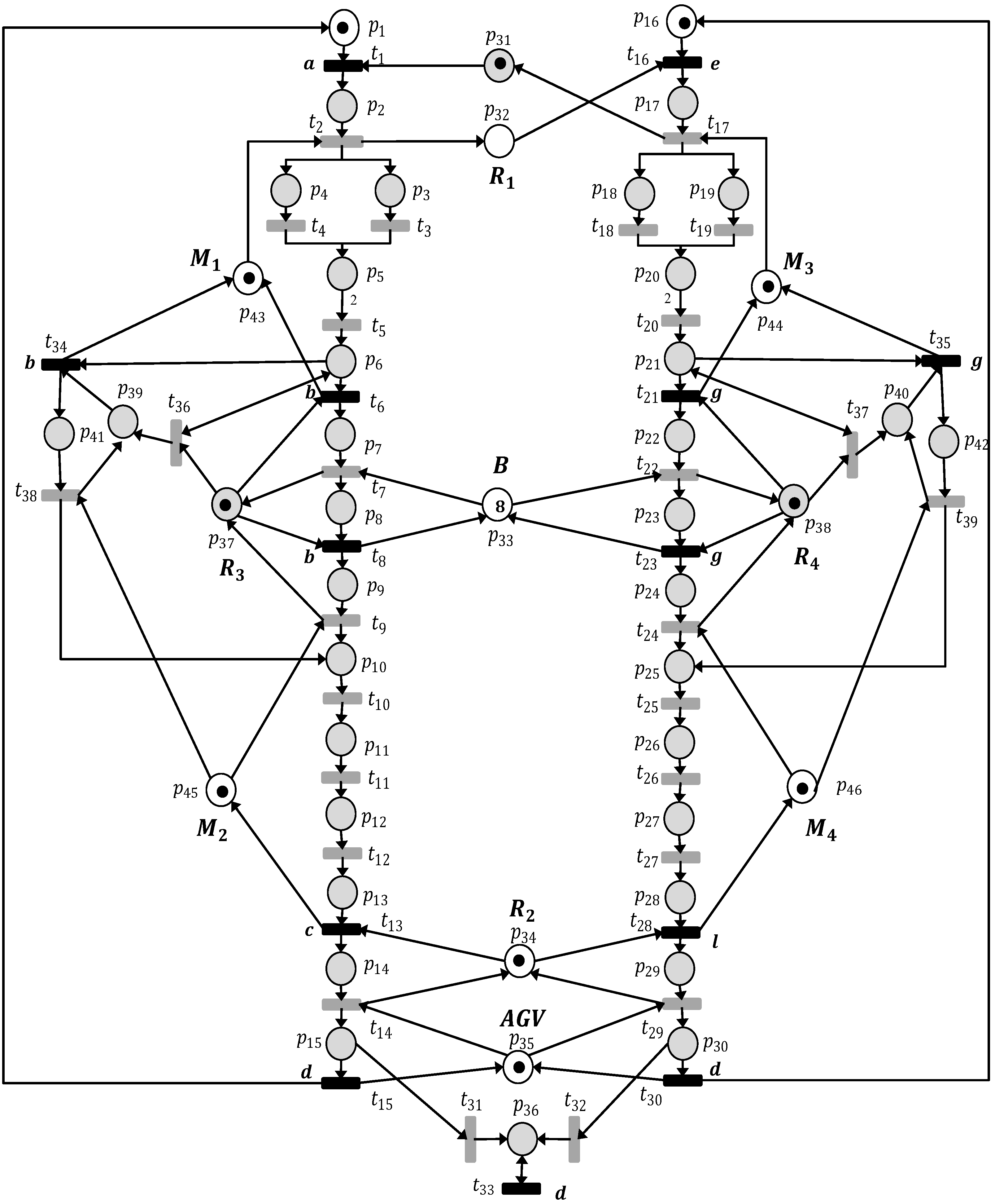
6. Experimental Results: A Manufacturing System

In this section, we exhibit the above results, using the example of an automated manufacturing system from [20], as shown in Figure 2. It contains 46 places and 39 transitions, including two inputs (I1 and I2), two outputs (O1 and O2), four machines (M1–M4), one buffer with finite capacity (B), and four robots (R1–R4). In [20], the operation of this system is discussed in detail. Assume that I1 and I2 each include a sensor that displays the number of items handled by the corresponding lines L1 and L2. Furthermore, sensors are installed on the machines (M1–M4), the two robots (R1 and R2), and the buffer (B), to indicate when an item is added. This PN might be considered as a POPN.
We have:
T d = { t 1 , t 2 , t 6 , t 7 , t 8 , t 9 , t 13 , t 14 , t 15 , t 16 , t 17 , t 21 , t 22 , t 23 , t 24 , t 28 , t 29 , t 30 , t 34 , t 35 , t 38 , t 39 } .
T ˜ u = { t 3 , t 4 , t 5 , t 10 , t 11 , t 12 , t 18 , t 19 , t 20 , t 25 , t 26 , t 27 , t 31 , t 32 , t 33 , t 36 , t 37 } .
Let L s = { σ 1 , σ 2 , σ 3 , σ 4 , σ 5 , σ 6 , σ 7 , σ 8 , σ 9 , σ 10 , σ 11 , σ 12 } be a secret language and O ( L s ) = { w 1 , w 2 , w 3 } be its associated secret observation sequences, as specified in Table 4 and Table 5, respectively. The results reported in this paper were obtained by solving (9) using CPLEX, which is a commercial Python library for linear programming optimization.
For G ( w 1 ) , there exists a sequence σ 1 = σ u 1 σ e 1 σ u 2 σ e 2 σ u 3 σ e 3 σ u 4 = t 1 t 2 t 3 t 4 t 5 t 6 enabled at M 0 , such that σ 1 L s and Λ ( ρ ( M 0 , σ 1 ) ) = w 1 , whose firing vectors σ u 1 = 0 , σ e 1 = b 1 , σ u 2 = 0 , σ e 2 = b 2 , σ u 3 = a 1 + a 2 + a 3 , σ e 3 = b 3 , σ u 4 = 0 satisfy (9), where a i and b i are called standard basis vectors for N n ˜ u and N n d , respectively, having all entries zero, except that the i t h entry equals 1. Notice that the solver takes into account the firing order of transitions, since σ has the same firing vector as the secret sequence t 1 t 2 t 4 t 3 t 5 t 6 .
For G ( w 2 ) , there exists a sequence σ 2 = σ u 1 σ e 1 σ u 2 σ e 2 σ u 3 σ e 3 σ u 4 = t 1 t 2 t 4 t 16 enabled at M 0 , such that σ 2 L s and Λ ( ρ ( M 0 , σ 2 ) ) = w 2 , whose firing vectors σ u 1 = 0 , σ e 1 = b 1 , σ u 2 = 0 , σ e 2 = b 2 , σ u 3 = a 2 , σ e 3 = b 10 , and σ u 4 = 0 satisfy (9).
For G ( w 3 ) , however, the ILP solver does not find any feasible solution, which implies the non-language opacity of the considered POPN.

7. LBO in Decentralized Setting

Modern networking technologies have rendered distributed systems increasingly more broadly used. These systems are composed of multiple networked components that communicate and coordinate actions, to achieve a common goal and appear to end-users as a single coherent entity. Figure 3 illustrates the privacy risks in an IoT-based smart house, where a set of intruders, distributed at different sites, are collecting sensing data and trying to deduce private information.

7.1. Decentralized Opacity with Coordinator

At this point, language-based opacity has been discussed in a centralized framework, where only a single intruder is trying to infer the system’s secret behavior. In this section, we consider decentralized settings, as shown in Figure 4, where a POPN is watched by a set of intruders J = { 1 , 2 , , n } who collaborate to verify, under a given observation sequence, if their language estimation is entirely contained in a secret. Formally, the system Q, with regard to the j t h intruder, can be described as follows:
Q j = ( N , M 0 , E j , V j , δ j ) is a POPN system, where N = ( P , T , P r e , P o s t ) and E j E is the set of observable labels by the j t h local intruder. As in the previous section, it holds that P = P o , j P u , j and P o , j P o ( P u , j = P P o , j ) comprise the set of locally observable (unobservable) places of intruder j. In addition, T = T o , j T u , j and T o , j T o ( T u , j = T T o , j ) comprise the set of locally observable (silent) transitions of intruder j. Moreover, we denote by T d , j T d ( T ˜ u , j = T T d , j ) the set of locally discernible (truly unobservable) transitions of intruder j. It holds that | P o , j | = m o , j , | P u , j | = m u , j , | T d , j | = n d , j and | T ˜ u , j | = n ˜ u , j . The matrices C ˜ u , j = P o s t ˜ u , j P r e ˜ u , j and C d , j = P o s t d , j P r e d , j , respectively, denote the restrictions of C to T ˜ u , j and T d , j .
The following assumptions are now introduced to this decentralized setting:
A1:
Each intruder has full understanding of the system’s structure and initial marking, but uses his own sensor configuration θ j = ( V j , δ j ) to track its evolution, where V j = ( v i k ) { 0 , 1 } m o , j × m , such that v i k = 1 if the i t h observable place by intruder j corresponds to place p k and to 0, otherwise, and where δ j is a local labeling function, such that δ j ( t ) = δ ( t ) if t T d , j and δ j ( t ) = ε , otherwise.
A2:
An observable place is observed by at least one local intruder, i.e., j J P o , j = P o .
A3:
A discernible transition is discerned by at least one local intruder, i.e., j J T d , j = T d .
A4:
Let be an ordering relation defined between sensor configurations, such that θ i θ j if intruder j observes more than intruder i, i.e., θ i θ j if T d , i T d , j P o , i P o , j .
Given M [ t M , a state transition, the obtained measurement with respect to a sensor configuration θ j associated with the jth local intruder is defined as follows:
ρ j ( M , t ) = ε p , if ( M ^ = M ^ ) ( δ j ( t ) = ε ) M ^ δ j ( t ) M ^ , otherwise .
Given σ = t 1 t 2 t h T * and M t 1 M 1 t 2 M 2 M h 1 t h M h , the evolution generated by firing σ at M, the measurement sequence associated with each local intruder j is defined as
ρ j ( M , σ ) = ρ j ( M , t 1 ) ρ j ( M 1 , t 2 ) ρ j ( M h 1 , t h ) = M ^ e 1 M ^ 1 M ^ 1 e 2 M ^ h o j 1 M ^ h o j 1 e h o j M ^ h o j ,
where e i E j { ε } , h o j h , and the associated local observation sequence for each intruder j is defined as w j = Λ ( ρ j ( M , σ ) ) = M ^ e 1 M ^ 1 e 2 M ^ h o j 1 e h o j M ^ h o j .
The firing sequences consistent with a local observation w j are denoted by S j ( w j ) = { σ T * | Λ ( ρ j ( M 0 , σ ) ) = w j } . As illustrated in Figure 4, after the firing of a transition sequence σ , each intruder j performs an event sequence estimation S j ( w j ) , using its local observation sequence w j , then sends it to a coordinator C. Based on the received information from all intruders, the coordinator evaluates its general estimation Γ ( w ) by finding the intersection of the received local estimations. Therefore, the coordination between intruders is called an intersection-based coordination protocol P .
Definition 8. 
An intersection-based coordination protocol P is defined by the following rules:
R1: 
The T u , j -induced subnet and the T o , j -induced subnet are acyclic for any local intruder j J .
R2: 
The general estimation is Γ ( w ) = j J S j ( w j ) .
R3: 
The more an intruder observes, the better its estimation will be, i.e., θ i θ j if, for all w O ( Q , M 0 ) , S j ( w j ) S i ( w i ) .
R4: 
The coordinator collects the event sequence estimation generated by each intruder without delay.
Remark 1. 
Let Q be a POPN, and P be an intersection-based coordination protocol; T d , c T d and P o , c P o are, respectively, the discernible transitions and observable places of Q, with regard to a coordinator C. Protocol P allows the coordinator to see the system’s original behavior: namely, T d , c = T d and P o , c = P o .
In detail, we have Γ ( w ) = j J S j ( w j ) ; then, for all w O ( Q , M 0 ) , Γ ( w ) S j ( w j ) , j J . We denote by θ c the sensor configuration of the coordinator. Under Rule R3, θ j θ c for j J ; thus, we can say that the coordinator observes more than all intruders j J . According to Assumption (A4), for all j J , we have T d , j T d , c and P o , j P o , c . As j J T d , j = T d and j J P o , j = P o , we have T d T d , c and P o P o , c . Consequently, T d , c = T d and P o , c = P o . Finally, we conclude that our coordination protocol allows the coordinator to see the system’s original behavior, by taking off the observation masks associated with intruders.
Now, let us characterize LBO in a decentralized setting with coordination: namely, co-language-based opacity (co-LBO).
Definition 9. 
Let Q = ( N , M 0 , E , V , δ ) be a POPN and L s L ( N , M 0 ) be a secret language. Q is co-LBO, with regard to L s , if and only if, for all w O ( L s ) , Γ ( w ) L s holds.
In simple terms, a PN system is co-LBO if it is language-opaque, with regard to the coordinator. Specifically, if two observations are indistinguishable for the coordinator, they are indistinguishable for any intruder j J .
Proposition 4. 
Let Q = ( N , M 0 , E , V , δ ) be a POPN and L s L ( N , M 0 ) be a secret language. If there is at least w O ( L s ) and j J , such that S j ( w j ) L s , then Q is not co-LBO, with regard to L s .
Proof. 
Let w O ( L s ) be a secret observation sequence. By Rule R2, we have Γ ( w ) = j J S j ( w j ) , which implies Γ ( w ) S j ( w j ) , j J . If there exists w O ( L s ) and j J , such that S j ( w j ) L s , then Γ ( w ) L s holds. Therefore, by Definition 9, Q is not co-LBO, with regard to L s . □
The main feature of investigating decentralized opacity consists in preventing a comprehensive computation of all possible sequences that could have fired. According to Proposition 4, if we find at least one intruder j, such that S j ( w j ) L s holds, then Q is not co-LBO, with regard to L s .
If there is no coordination between the intruders, we simply check the LBO for each intruder separately, as indicated in the previous sections. Accordingly, the achieved results can be extended from centralized to decentralized opacity. Therefore, we apply the results of Theorem 1 to each intruder j J as follows:
Let Q = ( N , M 0 , V , δ ) be a POPN and L s L ( N , M 0 ) be a secret language. Q is language-opaque, with regard to L s , if, for all w O ( L s ) , the following ILPP,
m i n f s . t . C ( M 0 , C d , j , C ˜ u , j , w j ) , j J NS ( M 0 , C d , j , C ˜ u , j , σ ) , σ L s
admits at least one feasible solution.
Definition 10. 
Let L s be a secret language, w = M ^ e 1 M ^ 1 e 2 M ^ h o 1 e h o M ^ h o ( h o 1 ) be a secret observation sequence, i.e., w O ( L s ) , and w j = M ^ e 1 M ^ 1 e 2 M ^ h o j 1 M ^ h o j 1 e h o j M ^ h o j ( h o j h o ) be the word projection of w, with regard to the local intruder j J . We define by J m a x ( w ) = { j J | h j h j , j J } the set of local intruders that can observe the maximum of w, called the maximal observers.
Proposition 5. 
Let Q = ( N , M 0 , E , V , δ ) be a POPN and L s L ( N , M 0 ) be a secret language. Q is co-LBO, with regard to L s , if and only if for each secret observation sequence w O ( L s ) and, for at least j J m a x ( w ) , there exists σ S ( w j ) L s ( w ) , such that for each local intruder j J , Λ ( ρ j ( M 0 , σ ) ) = w j .
Proof. 
(If) Suppose that, for all w O ( L s ) and for at least j J m a x ( w ) , there exists σ S ( w j ) L s ( w ) , such that for each local intruder j J , Λ ( ρ j ( M 0 , σ ) ) = w j . Consequently, σ is a non-secret transition sequence that is consistent with w j for j J (i.e., σ S ( w j ) , j J ).
We have Γ ( w ) = j J S j ( w j ) , and thus, σ Γ ( w ) L s ( w ) . Based on Proposition 4, Q is co-LBO, with regard to L s .
(Only if) Let us suppose that Q is co-LBO, with regard to L s , and for at least w O ( L s ) , and for each j J m a x ( w ) , there does not exist σ S ( w j ) L s , such that for each j J , Λ ( ρ j ( M 0 , σ ) ) = w j ; thus, j J S j ( w j ) L s . We have Γ ( w ) = j J S j ( w j ) L s and, therefore, Q is not co-LBO, with regard to L s , which opposes the hypothesis. □
Example 4. 
Consider the POPN in Figure 1. Let L s = { t 1 t 3 t 4 , t 1 t 3 t 2 t 5 , t 1 t 2 t 3 t 5 } be a secret language. Its associated secret observation sequences are given by O ( L s ) = { w 1 , w 2 } , where w 1 = [ 1 0 ] T a [ 0 1 ] T b [ 0 1 ] , w 2 = [ 1 0 ] T a [ 0 1 ] T [ 1 0 ] T , L s ( w 1 ) = { t 1 t 3 t 4 } , and L s ( w 2 ) = { t 1 t 3 t 2 t 5 , t 1 t 2 t 3 t 5 } . We have S ( w 1 ) = { t 1 t 3 t 4 , t 1 t 4 t 3 } and S ( w 2 ) = { t 1 t 2 t 3 t 5 , t 1 t 3 t 2 t 5 } . Let J = { 1 , 2 , 3 } be three local intruders satisfying Assumptions (A1–A4). Their observable places are P o , 1 = { p 1 } , P o , 2 = { p 1 , p 5 } , and P o , 3 = , respectively, and their discernible transitions are T d , 1 = { t 1 , t 5 } , T d , 2 = { t 1 } , and T d , 3 = { t 1 , t 5 } , respectively.
Based on the results reported in Table 6, we have:
J m a x ( w 1 ) = { 3 } ; then, we only need to consider the estimation of intruder 3, which is given by S 3 ( a b ) = { t 1 t 3 t 4 , t 1 t 4 t 3 , t 1 t 3 t 4 t 5 , t 1 t 4 t 3 t 5 } . We have t 1 t 4 t 3 L s , Λ ( ρ 1 ( M 0 , t 1 t 4 t 3 ) ) = [ 1 ] a [ 0 ] and Λ ( ρ 2 ( M 0 , t 1 t 4 t 3 ) ) = [ 1 0 ] T [ 0 1 ] T ; then, w 1 is co-LBO, with regard to L s .
J m a x ( w 2 ) = { 1 , 2 } . Since intruders 1 and 2 observe two discernible transitions, while intruder 3 only observes one discernible transition, then we only need to consider the estimation of either intruder 1 or 2. Let us consider the estimation of intruder 2, which is given by S 2 ( [ 1 0 ] T [ 0 1 ] T [ 1 0 ] T ) = { t 1 t 2 t 3 t 5 , t 1 t 4 t 3 t 5 , t 1 t 3 t 2 t 5 , t 1 t 3 t 4 t 5 } . We have S 2 ( w 2 ) L s ( w 2 ) = { t 1 t 4 t 3 t 5 , t 1 t 3 t 4 t 5 } . For intruder 3, Λ ( ρ 3 ( M 0 , t 1 t 3 t 4 t 5 ) ) = Λ ( ρ 3 ( M 0 , t 1 t 4 t 3 t 5 ) ) = a b a , then w 2 is not co-LBO, with regard to L s .

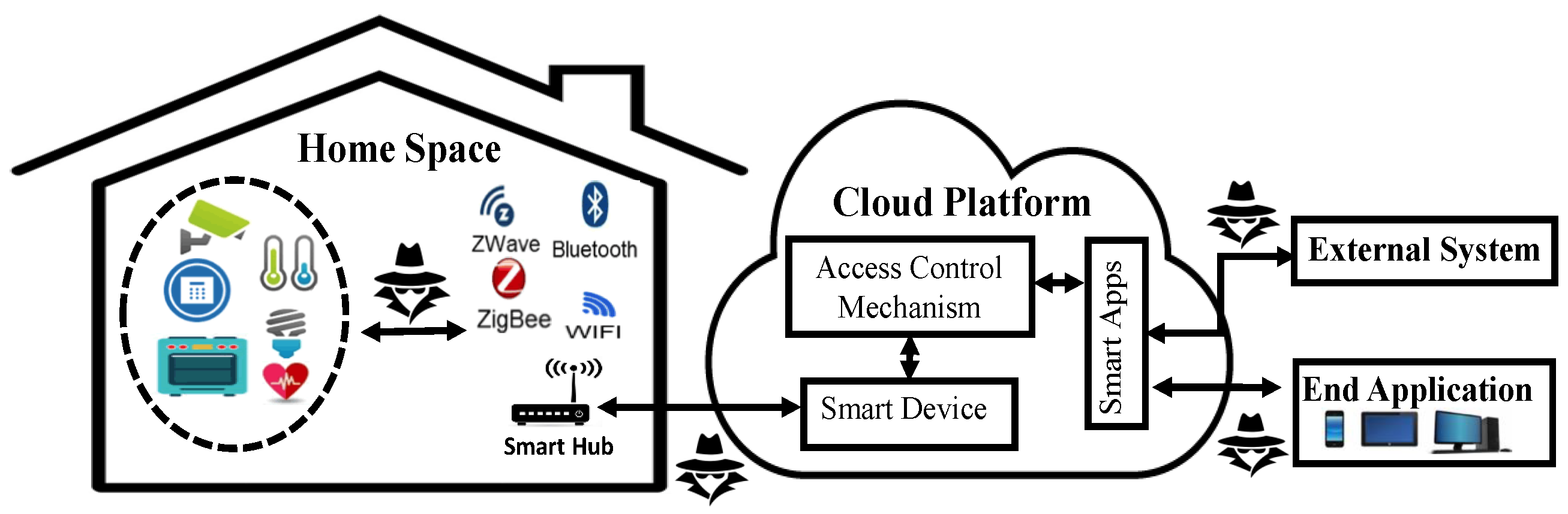
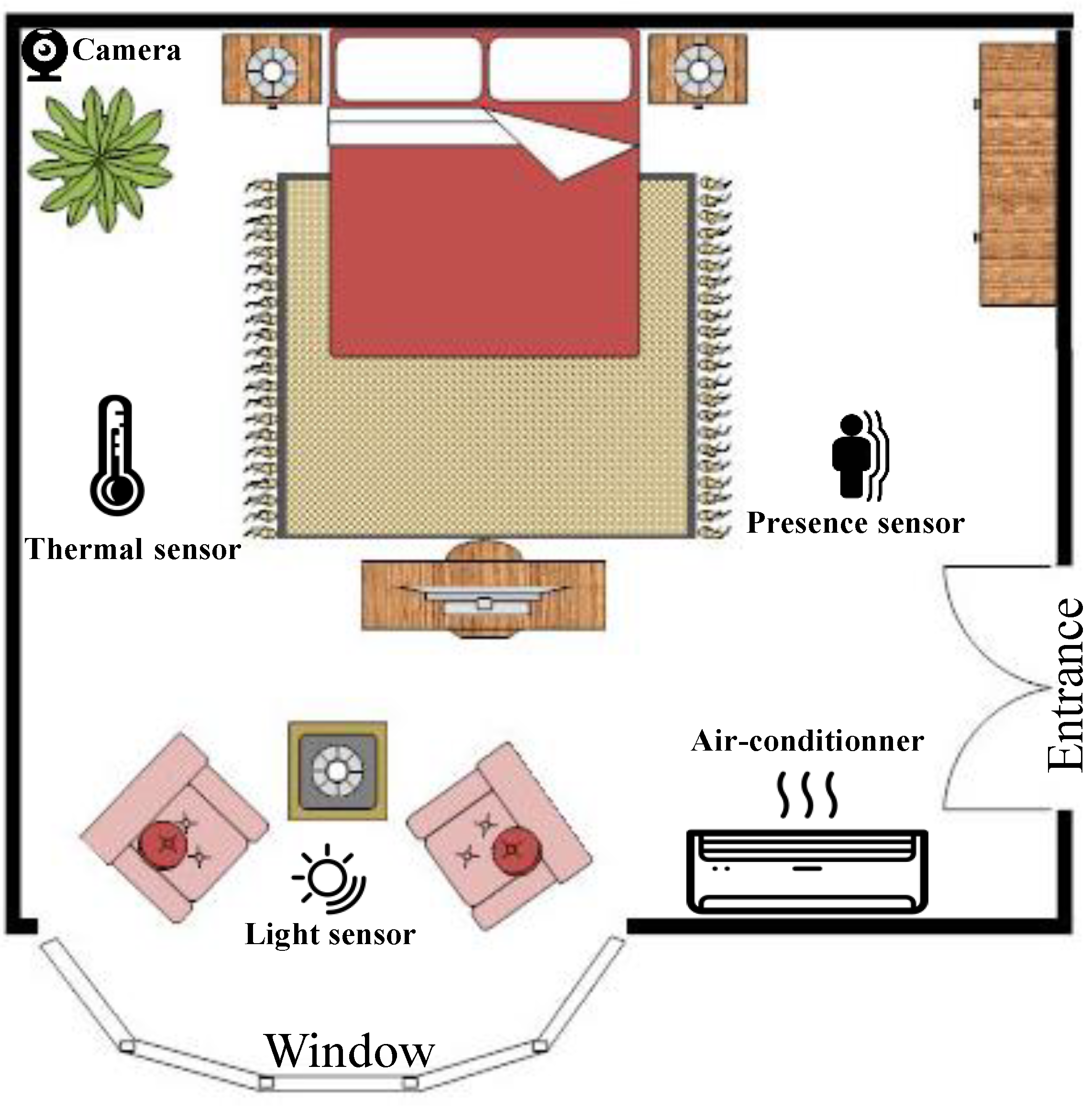
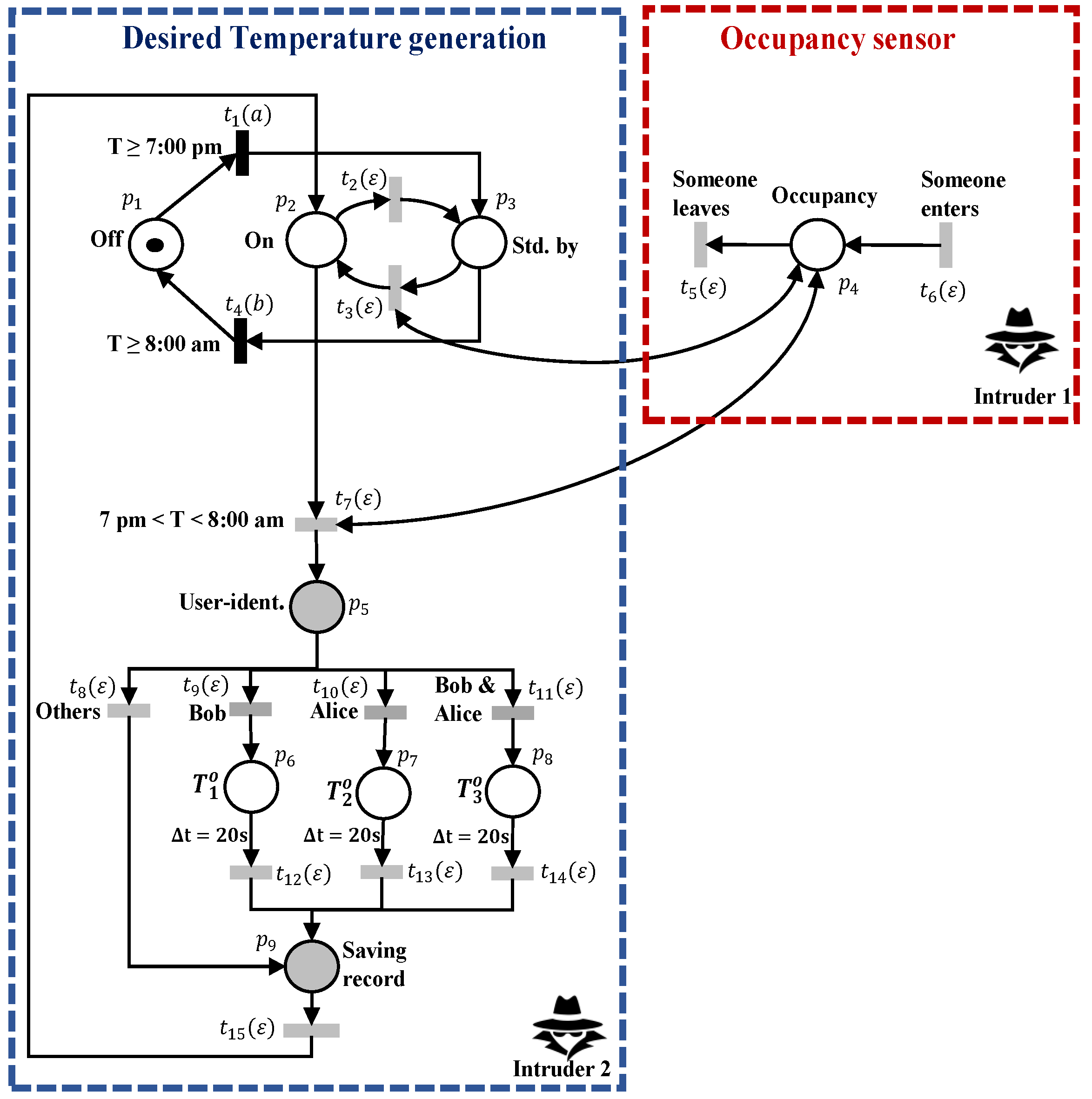
7.2. Study Case: Temperature Control System

Modern inference techniques, such as machine learning algorithms, can provide enough data to infer user activities, including house occupancy, sleeping patterns, and work schedules. For instance, innocuous data, such as in-home temperatures, could violate the user’s privacy of location, which is the right of individuals to be present in a space without being tracked or monitored or without anyone knowing where they are.
We use a smart thermostat as a case study, which controls the heating and air conditioning in Alice and Bob’s bedroom, shown in Figure 5. The bedroom mainly includes one bed, a window, a door, an air conditioner (AC), a smart thermostat connected to an HVAC (heating, ventilation, and air conditioning) system, a camera, and sensors to measure the necessary data. The thermostat allows for creating a heating and cooling schedule during the day, to save energy. It can also use sensors to check room occupancy, and it automatically sets itself to a standby temperature when the room is empty. The thermostat temperature-control system is modeled by a POPN, as shown in Figure 6. The system turns off (place p 1 ) at 8:00 a.m. (transition t 4 ), when Bob and Alice are outside for work, and starts around 7:00 p.m. (transition t 1 ), then goes directly into a standby state (place p 3 ), which prepares the room for the arrival of Bob and Alice in the evening. From this time on, the system is either in an ON state (place p 2 ), when the presence sensor detects someone inside the room (place p 4 ) or in a Standby state, when the presence sensor does not detect anyone inside the room. Note that the token number in place p 5 indicates the number of persons inside the bedroom. When the system goes into the ON state, a quick user identification process starts (place p 5 ), based on a smart facial recognition camera powered by artificial intelligence and placed in the room’s upper left corner. At the end of this process, there are four possibilities:
  • Bob is identified (transition t 9 ); then, his preferred reference temperature T 1 o (place p 6 ) will be displayed.
  • Alice is identified (transition t 10 ) in the room. In this case, the preferred reference temperature will be T 2 o (place p 7 ).
  • Bob and Alice are simultaneously present in the room (transition t 11 ); then, the reference temperature T 3 o (place p 8 ), on which Bob and Alice have agreed, will be displayed.
  • Neither Bob nor Alice is identified (transition t 8 ).
The chosen temperature will remain activated for a duration of 20 s (transitions t 12 , t 13 , t 14 ). At the end of this period, the system saves a temperature record (place p 9 ), to keep track of the user’s schedule and habits, and it then programs itself to match his temperature patterns.
Now, let us check whether intruders can violate Bob and Alice’s privacy of location. Let the secret information be
“Alice is alone inside the bedroom”.
Intruder 1 is observing the occupancy sensor’s activity, and intruder 2 is observing the thermostat’s activity. We have:
T d , 1 = { t 5 , t 6 }
T ˜ u , 1 = { t 1 , t 2 , t 3 , t 4 , t 7 , t 8 , t 9 , t 10 , t 11 , t 12 , t 13 , t 14 , t 15 }
T d , 2 = { t 2 , t 3 , t 7 , t 9 , t 10 , t 11 , t 12 , t 13 , t 14 , t 15 , t 1 , t 4 }
T ˜ u , 2 = { t 5 , t 6 , t 8 } .
When Alice enters the bedroom at 7:30 pm, transition sequence t 1 t 6 t 3 t 7 t 8 fires, and intruder 1 observes w 1 = [ 0 ] [ 1 ] , which makes him conclude that someone is alone inside the room, but he is not sure whether it is Alice or not.
On the other hand, intruder 2 observes w 2 = [ 100000 ] T a [ 001000 ] T [ 010000 ] T [ 000000 ] T [ 000010 ] T , and the presence of a token in places p 7 indicates that Alice is inside the room, but intruder 2 is not sure whether she is alone or not. We check the opacity for each intruder separately, using Theorem 1. We find that both ILPPs G ( w 1 ) and G ( w 2 ) admit a feasible solution. Therefore, the temperature-control system is LBO, with regard to to intruders 1 and 2. However, there is no solution available for ILPP (10). Consequently, the coordination between intruders 1 and 2 can disclose the secret information and infer that Alice is alone inside the room.

8. Conclusions and Future Work

The formulation and verification of LBO in the context of DESs modeled with POPNs were discussed in this research. We provided a necessary and sufficient condition for LBO verification, based on a mathematical description of a net system. Specifically, we proposed linear constraints to check the consistency and non-secrecy aspects of transition sequences. Moreover, these findings were extended to encompass scenarios of decentralized opacity. In these scenarios, the system was examined by multiple intruders, who subsequently shared their observation outcomes with a coordinator, in order to disclose a secret behavior. The proposed approach is more general and scalable than the existing methods for LBO verification in LPNs, as it can be applied to both bounded and unbounded POPNs without requiring any expensive offline computation.
Our future study will extend the proposed ILP-based approach to fault diagnosis in a POPN. Furthermore, it would be of interest to investigate other security problems and potential vulnerabilities, such as unauthorized access, cyber-attacks, intrusion detection, prevention, etc.

Author Contributions

Methodology, I.S. and A.L.; software, A.L.; formal analysis, H.D.; resources, A.M.E.-S.; supervision, Z.L. All authors have read and agreed to the published version of the manuscript.

Funding

This work was partially supported by the Guangzhou Innovation and Entrepreneurship Leading Team Project Funding under Grant No. 202009020008 and the Science and Technology Fund, FDCT, Macau SAR, under Grant 0064/2021/A2. The authors extend their appreciation to King Saud University, Saudi Arabia, for funding this work through Researchers Supporting Project number (RSP2023R133), King Saud University, Riyadh, Saudi Arabia.

Data Availability Statement

Not applicable.

Conflicts of Interest

The authors declare no conflict of interest.

References

  1. Gaudin, B.; Marchand, H. Supervisory control and deadlock avoidance control problem for concurrent discrete event systems. In Proceedings of the 44th IEEE Conference on Decision and Control, Seville, Spain, 12–15 December 2005; pp. 2763–2768. [Google Scholar]
  2. Jiao, T.; Wonham, W. Composite supervisory control for symmetric discrete-event systems. Int. J. Control 2020, 93, 1630–1636. [Google Scholar] [CrossRef]
  3. Bryans, J.W.; Koutny, M.; Mazaré, L.; Ryan, P.Y. Opacity generalised to transition systems. In Proceedings of the International Workshop on Formal Aspects in Security and Trust, Newcastle upon Tyne, UK, 18–19 July 2005; pp. 81–95. [Google Scholar]
  4. Basile, F.; De Tommasi, G.; Sterle, C. Non-interference enforcement in bounded Petri nets. In Proceedings of the 2018 IEEE Conference on Decision and Control (CDC), Miami Beach, FL, USA, 17–19 December 2018; pp. 4827–4832. [Google Scholar]
  5. Lin, F. Opacity of discrete event systems and its applications. Automatica 2011, 47, 496–503. [Google Scholar] [CrossRef]
  6. Lafortune, S.; Lin, F.; Hadjicostis, C.N. On the history of diagnosability and opacity in discrete event systems. Annu. Rev. Control 2018, 45, 257–266. [Google Scholar] [CrossRef]
  7. Saadaoui, I.; Li, Z.; Wu, N. Current-state opacity modelling and verification in partially observed Petri nets. Automatica 2020, 116, 108907. [Google Scholar] [CrossRef]
  8. Ben-Kalefa, M.; Lin, F. Opaque superlanguages and sublanguages in discrete event systems. Cybern. Syst. 2016, 47, 392–426. [Google Scholar] [CrossRef]
  9. Badouel, E.; Bednarczyk, M.; Borzyszkowski, A.; Caillaud, B.; Darondeau, P. Concurrent secrets. Discret. Event Dyn. Syst. 2007, 17, 425–446. [Google Scholar] [CrossRef]
  10. Tong, Y.; Ma, Z.; Li, Z.; Seactzu, C.; Giua, A. Verification of language-based opacity in Petri nets using verifier. In Proceedings of the American Control Conference, Boston, MA, USA, 6–8 July 2016; pp. 757–763. [Google Scholar]
  11. Cong, X.; Fanti, M.P.; Mangini, A.M.; Li, Z. On-line verification of current-state opacity by Petri nets and integer linear programming. Automatica 2018, 94, 205–213. [Google Scholar] [CrossRef]
  12. Wu, Y.C.; Lafortune, S. Comparative analysis of related notions of opacity in centralized and coordinated architectures. Discret. Event Dyn. Syst. 2013, 23, 307–339. [Google Scholar] [CrossRef]
  13. Basile, F.; De Tommasi, G. An algebraic characterization of language-based opacity in labeled Petri nets. IFAC-PapersOnLine 2018, 51, 329–336. [Google Scholar] [CrossRef]
  14. Paoli, A.; Lin, F. Decentralized opacity of discrete event systems. In Proceedings of the 2012 American Control Conference (ACC), Montreal, QC, Canada, 27–29 June 2012; pp. 6083–6088. [Google Scholar]
  15. Lin, F.; Wonham, W.M. Decentralized supervisory control of discrete-event systems. Inf. Sci. 1988, 44, 199–224. [Google Scholar] [CrossRef]
  16. Ramadge, P.J.; Wonham, W.M. The control of discrete event systems. Proc. IEEE 1989, 77, 81–98. [Google Scholar] [CrossRef]
  17. Tripakis, S.; Rudie, K. Decentralized Observation of Discrete-Event Systems: At Least One Can Tell. IEEE Control Syst. Lett. 2022, 6, 1652–1657. [Google Scholar] [CrossRef]
  18. Saadaoui, I.; Li, Z.; Wu, N.; Khalgui, M. Depth-first search approach for language-based opacity verification using Petri nets. IFAC-PapersOnLine 2020, 53, 378–383. [Google Scholar] [CrossRef]
  19. Silva, M.; Terue, E.; Colom, J.M. Linear algebraic and linear programming techniques for the analysis of place/transition net systems. In Proceedings of the Advanced Course on Petri Nets, Dagstuhl, Germany, 7–18 October 1996; pp. 309–373. [Google Scholar]
  20. Cabasino, M.P.; Giua, A.; Pocci, M.; Seatzu, C. Discrete event diagnosis using labeled Petri nets. An application to manufacturing systems. Control Eng. Pract. 2011, 19, 989–1001. [Google Scholar] [CrossRef]
Figure 1. A POPN, where unobservable transitions and places are depicted by gray bars and circles, respectively.
Mathematics 11 03880 g001
Figure 2. An automated manufacturing system’s Petri net model.
Mathematics 11 03880 g002
Figure 3. Privacy risks of Iot-based smart houses.
Mathematics 11 03880 g003
Figure 4. The decentralized architecture.
Mathematics 11 03880 g004
Figure 5. Bedroom layout.
Mathematics 11 03880 g005
Figure 6. PN-based temperature generator.
Mathematics 11 03880 g006
Table 1. Integer variables of ILPP G ( w ) .
VariableTypeSizeRangeTotal
σ u i Integer n ˜ u × 1 i { 1 , , h o + 1 } n ˜ u · ( h o + 1 )
σ e j Integer n d × 1 i { 1 , , h o + 1 } n d · h o
z i k + Integer 1 × 1 i { 1 , , h o + 1 } k ∈ {1, …, n ˜ u } n ˜ u · ( h o + 1 ) · η
z i k Integer 1 × 1 i { 1 , , h o + 1 } k ∈ {1, …, n ˜ u } n ˜ u · ( h o + 1 ) · η
q j k + Integer 1 × 1 i { 1 , , h o + 1 } k ∈ {1, …, nd} n d · h o · η
q j k Integer 1 × 1 i { 1 , , h o + 1 } k ∈ {1, …, nd} n d · h o · η
a i k Binary 1 × 1 i { 1 , , h o + 1 } k ∈ {1, …, n ˜ u } n ˜ u · ( h o + 1 ) · η
b j k Binary j × 1 i { 1 , , h o + 1 } k ∈ {1, …, nd} n d · h o · η
UInteger 1 × 1 1 1 · η
M i 1 Integer m × 1 i { 1 , , h o + 1 } m · ( h o + 1 ) · η
x i k Binary n ˜ u × 1 i { 1 , , h o + 1 } k ∈ {1, …, Li} n ˜ u · ( h o + 1 ) · L i · η
v i Integer 1 × 1 i { 1 , , h o + 1 } ( h o + 1 ) · η
y 1 Binary 1 × 1 1 1 · η
y 2 Binary 1 × 1 1 1 · η
y 3 Binary 1 × 1 1 1 · η
Table 2. Constraints of ILPP G ( w ) .
Constraint SetSub-ConstraintsExtentRangeTotal
f1111
C ( M 0 , C d , C ˜ u , w ) 3.am1m
3.bm l { 1 h o } m · h o
3.c m o i { 1 h o + 1 }
j ∈ {1 … ho}
m o · ( h o + 1 )
mo·ho
3.d2 j { 1 h o } 2 · h o
NS ( M 0 , C d , C ˜ u , σ ) σ L s ( w ) 8.a1 n ˜ u i { 1 h o + 1 } n ˜ u · ( h o + 1 ) · η
8.b1 n d j { 1 h o } n d · h o · η
8.a211 1 · η
8.b211 1 · η
8.a32 i { 1 h o + 1 }
k {1 …nu}
2 · n ˜ u · ( h o + 1 ) · η
8.b32 j { 1 h o }
k {1 …nd}
2 · n d · h o · η
8.c1m i { 1 h o + 1 } n ˜ u · ( h o + 1 ) · η
8.c2m i { 1 h o + 1 }
r ∈ {1 … Li}
m · L i ( h o + 1 ) · η
8.c31 i { 1 h o + 1 } ( h o + 1 ) · η
8.c41 i { 1 h o + 1 } ( h o + 1 ) · η
8.c511 1 · η
8.d11 1 · η
Table 3. LBO verification approaches.
FrameworkGraphSecret NatureComplexity
 [5]AutomatonNoLabelsExponential
 [10]LPNYesObservable transitionsExponential
 [13]LPNNoLabelsNP-hard
Proposed approachPOPNNoTransitionsNP-hard
Table 4. Secret transition sequences.
σ i Value L s ( σ )
σ 1 t 1 t 2 t 4 t 3 t 5 t 6 w 1
σ 2 t 1 t 2 t 16 w 2
σ 3 t 1 t 2 t 16 t 3 , t 1 t 2 t 3 t 4 t 5 t 36 t 16 w 2
σ 4 t 1 t 2 t 3 t 4 t 5 t 16 , t 1 t 2 t 3 t 4 t 16 t 5 w 2
σ 5 t 1 t 2 t 3 t 4 t 5 t 36 t 34 w 1
σ 6 t 1 t 2 t 3 t 4 t 5 t 16 t 36 w 2
σ 7 t 1 t 2 t 3 t 4 t 16 w 2
σ 8 t 1 t 2 t 3 t 4 t 16 t 5 t 36 w 2
σ 9 t 1 t 2 t 16 t 3 t 4 t 5 w 2
σ 10 t 1 t 2 t 16 t 3 t 4 w 2
σ 11 t 1 t 2 t 16 t 3 t 4 t 5 t 36 w 2
σ 12 t 1 t 2 t 3 t 4 t 5 t 6 t 7 t 8 t 9 t 10 t 11 t 12 t 13 w 3
Table 5. Secret observation sequences.
w i Value
w 1 [ 1108111111 ] T a [ 0108111111 ] T [ 0118110111 ] T b [ 0118111111 ] T
w 2 [ 1108111111 ] T a [ 0108111111 ] T [ 0118110111 ] T e [ 0008110111 ] T
w 3 [ 1108111111 ] T a [ 0108111111 ] T [ 0118110111 ] T b [ 0118111111 ] T
[ 0117111111 ] T b [ 0118111111 ] T [ 0118111101 ] T c [ 0118011111 ] T
Table 6. Secret words associated with each intruder.
IntruderProjection of w 1 Projection of w 2
1 [ 1 ] a [ 0 ] [ 1 ] a [ 0 ] [ 1 ]
2 [ 1 0 ] T [ 0 1 ] T [ 1 0 ] T [ 0 1 ] T [ 1 0 ] T
3 a b a
Disclaimer/Publisher’s Note: The statements, opinions and data contained in all publications are solely those of the individual author(s) and contributor(s) and not of MDPI and/or the editor(s). MDPI and/or the editor(s) disclaim responsibility for any injury to people or property resulting from any ideas, methods, instructions or products referred to in the content.

