Asymptotic Normality of M-Estimator in Linear Regression Model with Asymptotically Almost Negatively Associated Errors

Abstract

This paper studies a linear regression model in which the errors are asymptotically almost negatively associated (AANA, in short) random variables. Firstly, the central limit theorem for AANA sequences of random variables is established. Then, we use the central limit theorem to investigate the asymptotic normality of the M-estimator for the unknown parameters. Some results for independent and negatively associated (NA, in short) random variables are extended to the case of AANA setting. Finally, a simulation is carried out to verify the asymptotic normality of the M-estimator in the model.

1. Introduction

A lot of researchers have derived the asymptotic properties of the estimators in linear regression models with independent random errors, which are not reasonable in many applications. Therefore, it is of great significance to study linear regression models with dependent errors.

Consider the following linear regression model:

$$Y_i={x_i}^{\prime }{\beta }_0+e_i, \left(1\le i\le n,n\ge 1\right),$$

(1)

where ${\beta }_0$ is an unknown $p\times 1$ regression parameter vector, $x_i=({x_i}_1,x_{i2},\dots ,x_{ip}{)}^{\prime }$ is a known $p\times 1$ explanatory vector, $\left\{Y_i\right\}$ are the scalar response variables, and the errors $\left\{e_i\right\}$ are asymptotically almost negatively associated random variables.

In many situations, the assumption that random variables are independent is not suitable, so people often study dependent random variables. AANA random variables are widely used. Independent and NA random variables are special AANA random variables. The concept of AANA sequences was proposed by Chandra and Ghosal [1].

Definition 1

([1]). A random sequence $\left\{X_n,n\ge 1\right\}$ is said to be asymptotically almost negatively associated (AANA, in short) if a non-negative sequence $q\left(n\right)\to 0$ $\left(n\to \infty \right)$ exists, such that:

$$Cov\left(f\left(X_n\right),g\left(X_{n+1},X_{n+2},\cdots ,X_{n+k}\right)\right)\le q\left(n\right){\left(Var\left(f\left(X_n\right)\right)Var\left(g\left(X_{n+1},X_{n+2},\cdots ,X_{n+k}\right)\right)\right)}^{1/2},$$

for all $n,k\ge 1$ and for all coordinate wise non-decreasing continuous functions $f$ and $g$ whenever variances exist. $\left\{q\left(n\right),n\ge 1\right\}$ refers to the mixing coefficients.

Many results on the AANA sequences of random variables have been achieved. The family of AANA sequences contains NA (in particular, independent) sequences (with $q\left(n\right)=0,n\ge 1$) and some more random sequences (see [1]). The following two examples are AANA sequences but not NA: ${\xi }_n={\left(1+a_n^2\right)}^{-1/2}\left({\eta }_n+a_n{\eta }_{n+1}\right)$ (see [1]) and ${\zeta }_n={\eta }_n+a_n{\eta }_{n+1}$ (see [2]), where ${\eta }_1,{\eta }_2,\dots$ are $i.i.d.$ $N\left(0,1\right)$ random variables, $a_n>0$ and $a_n\to 0$ as $n\to \infty$. Some Rosenthal-type inequalities for AANA sequences are obtained in [3]. More studies on AANA sequences of random variables can be found in [4,5,6].

M-estimation include LS and LAD estimation as special cases. In order to investigate the location parameter model, Huber [7] first introduced M-estimation. Huber [8] extended M-estimation to a generalized linear model and proposed the following definition.

Definition 2

([8]). Assume that $\rho (\cdot )$ is some suitable function on $R^1$. The M-estimator ${\widehat{\beta }}_n$ of ${\beta }_0$ is defined by:

$${\widehat{\beta }}_n=\arg \underset{{\beta }_0\in R^p}{\min }{\displaystyle \sum _{i=1}^n\rho \left(Y_i-x_i^{\prime }{\beta }_0\right)}.$$

(2)

A series of useful results using M-estimation have been derived by various researchers. Under independent errors, the consistency and asymptotic normality, the methods and theories of linear hypothesis testing, and the linear representation of the M-estimator were discussed more comprehensively in [9,10,11,12,13]. Wu [14] studied the consistency of the M-estimator in a linear model with NA errors. More studies on M-estimation can be found in [15,16,17,18].

However, we have not found studies which focus on the asymptotic normality of the M-estimator in a linear regression model whose errors are AANA in the literature. Therefore, this article considers the linear regression model with AANA errors. The main novelties of this paper are as follows. Firstly, we use moment inequalities to establish the central limit theorem for AANA sequences, which extend the corresponding results for NA sequences to AANA sequences. Secondly, we use the central limit theorem to study the asymptotic normality of the M-estimators of the unknown parameters. The results extend the corresponding ones for independent and some dependent errors. At last, we carried out a simulation to verify the validity of the results.

The remainder of this paper is organized as follows. In Section 2, the central limit theorem for AANA random sequences is derived. In Section 3, the asymptotic normality of the M-estimators of unknown parameters is investigated under some mild conditions. In Section 4, a simulated study is presented to support the results. In Section 5, we conclude the paper.

In the paper, let $C$ be a positive constant whose values may vary at different places. $i.i.d.$ stands for independent and identically distributed. $x^{+}=\max \left\{0,x\right\}$ and $x^{-}=\max \left\{0,-x\right\}$. $\stackrel{\wedge}{=}$ means “defined as”. $\Vert \cdot \Vert$ is the Euclidean norm.

2. Central Limit Theorem for AANA Random Sequences

To derive the asymptotic normality of M-estimators of unknown parameters, we give an important conclusion in this section first and call it the central limit theorem for AANA random sequences.

Theorem 1.

Assume that $\left\{X_n;n\ge 1\right\}$ is an identically distributed AANA random sequence with mixing coefficients $\{q(n),n\ge 1\}$ and the following conditions are satisfied:

• (A₁) $E{X}_1=0$, $0<E{X}_1^2<\infty$;
• (A₂)

  $$\underset{n\to \infty }{\lim }E S_n^2/n={\sigma }^2;$$

  (3)
• (A₃) there exists a strictly increasing natural numbers sequence $\left\{n_k\right\}$, for $0<\alpha \le 1$, such that:

  $${{\displaystyle \sum _{k=1}^{\infty }\left(\frac{m_k}{n_k}\right)}}^{1+\alpha /2}<\infty \mathrm{and} \underset{k\to \infty }{\lim }\frac{1}{m_k}E{S}_{n_{k-1},m_k}^2={\sigma }^2;$$

  (4)
• (A₄) ${\displaystyle \sum _{n=1}^{\infty }q(n)}=h<\infty$; Then,

  $$\frac{S_n}{\sqrt{E{S}_n^2}}\stackrel{d}{\to }N\left(0,1\right),$$

  (5)

  where $n_0=0$, $m_k=n_k-n_{k-1}\left(k\ge 1\right)$, $S_{m,n}={\displaystyle \sum _{j=1}^n{X}_{j+m}}$, $S_n=S_{0,n}$, and $\stackrel{d}{\to }$ stands for convergence in distribution.

Remark 1.

In Theorem 1, except for the extra condition ($A_4$), other conditions are the same as that of Theorem 2.2 in Su and Chi [19].

As independent and NA sequences are special AANA sequences, we can easily obtain the following corollaries.

Corollary 1.

Let $\left\{X_n;n\ge 1\right\}$ be an $i.i.d.$ random sequence, as the conditions ($A_1$)–($A_3$) are satisfied, and then conclusion (5) holds.

Corollary 2

([19]). Let $\left\{X_n;n\ge 1\right\}$ be an identically distributed NA random sequence, as the conditions ($A_1$)–($A_3$) are satisfied, and then conclusion (5) holds.

To prove Theorem 1, we need the following lemmas.

Lemma 1

([3]). If $\left\{X_n,n\ge 1\right\}$ is an AANA sequence whose mixing coefficients are $\{q(n),n\ge 1\}$, then so is $\{f_n(X_n),n\ge 1\}$, where $f_1,f_2,\cdots$ are non-increasing or non-decreasing functions.

Lemma 2

([3]). Let $\left\{X_n,n\ge 1\right\}$ be an AANA sequence of zero mean with mixing coefficients $\{q(n),n\ge 1\}$, then there exists a positive constant $C_p$ depending only on $p$, such that:

$$E\left(\underset{1\le i\le n}{\max }{\left|T_i\right|}^p\right)\le C_p\left\{{\displaystyle \sum _{i=1}^{n}E{\left|X_i\right|}^p+{\left({\displaystyle \sum _{i=1}^{n-1}{q}^{2/m}\left(i\right){\Vert X_i\Vert }_p}\right)}^2}\right\},$$

for any $n$ and $1<p\le 2$, where $T_i={\displaystyle \sum _{j=1}^i{X}_j}, {\Vert X_i\Vert }_p={\left(E{\left|X_i\right|}^p\right)}^{1/p}, m=p/\left(p-1\right)$.

Lemma 3

([20]). Let $\left\{X_n,n\ge 1\right\}$ be an $i.i.d.$ random sequence with $E{X}_j=0$ and $E{\left|X_j\right|}^{2+\alpha }<\infty$ for $0\le \alpha \le 1$ and all $j\ge 1$. Assume that $f:R\to R$ is twice derivative and ${\Vert f^{″}\Vert }_{\alpha }<\infty$. Then,

$$\left|Ef\left(S_n/s_n\right)-{\displaystyle \int fd\Phi }\right|\le c{\Vert f^{″}\Vert }_{\alpha }{s_n}^{-2-\alpha }{\displaystyle \sum _{j=1}^{n}E{\left|X_j\right|}^{2+\alpha }},$$

where $s_n={\left(E{S}_n^2\right)}^{1/2}={\left({\displaystyle \sum _{j=1}^{n}E{X}_j^2}\right)}^{1/2}$ and $\Phi$ is the standard normal distribution function.

Lemma 4

([21]). If $\left\{X_n,n\ge 1\right\}$ is an AANA sequence with zero mean and mixing coefficients $\{q(n),n\ge 1\}$, satisfying ${\sigma }_n^2\stackrel{\wedge}{=}E{X}_n^2<\infty$, $n\ge 1$, then

$$E{S}_n^2\le 2{\displaystyle \sum _{i=1}^n{\sigma }_i^2}+4{\left({\displaystyle \sum _{i=1}^{n-1}q\left(i\right){\sigma }_i}\right)}^2,$$

where $S_n={\displaystyle \sum _{i=1}^n{X}_i}$.

Lemma 5.

Let $\left\{X_n,n\ge 1\right\}$ be an AANA sequence with mixing coefficients $\{q(n),n\ge 1\}$. Assume that $h_1\left(x\right)$ and $h_2\left(y\right)$ are absolutely continuous, bounded and real on $R$ with $\left|h_1\left(x\right)\right|\le C$ and $\left|h_2\left(y\right)\right|\le C$. Then,

$$\begin{array}{l} \left|Cov\left[h_1\left(X_n\right),h_2\left(g\left(X_{n+1},X_{n+2},\cdots ,X_{n+k}\right)\right)\right]\right|\\ \le C\left[-Cov\left(X_n,g\left(X_{n+1},X_{n+2},\cdots ,X_{n+k}\right)\right)+q\left(n\right){\Vert X_n\Vert }_{2,1}{\Vert g\left(X_{n+1},\cdots ,X_{n+k}\right)\Vert }_{2,1}\right]\end{array}$$

for all $n,k\ge 1$ and for all coordinate wise non-decreasing continuous functions $g$ whenever the variances exist, where ${\Vert X\Vert }_{2,1}={\displaystyle {\int }_0^{\infty }{\left(P\left(\left|X\right|\ge x\right)\right)}^{\frac{1}{2}}}dx$.

Proof. 

The proof is similar to that of the Lemma 3.5 in Zhang [22], with $q\left(n\right)$ taking the place of its ${\rho }^{-}\left(X,Y\right)$. We omit the details here. □

Lemma 6.

Let $\left\{X_n,n\ge 1\right\}$ be an AANA sequence with mixing coefficients $\left\{q\left(n\right),n\ge 1\right\}$. If $E{\left|X_j\right|}^2<\infty$, then

$$\left|E{\displaystyle \prod _{j=1}^n{e}^{i{\lambda }_j{X}_j}}-{\displaystyle \prod _{j=1}^{n}E{e}^{i{\lambda }_j{X}_j}}\right|\le C{\displaystyle \sum _{1\le j<\ne l\le n}\left|{\lambda }_j{\lambda }_{l}Cov\left(X_j,X_l\right)\right|}+C{\displaystyle \sum _{j=1}^{n-1}q\left(j\right)}$$

for any real ${\lambda }_j$, $j=1,\cdots ,n$.

Proof. 

We proceed the proof by induction on $n$. The result is true for $n=1$ trivially and is true for $n=2$ by Lemma 5 and ${\Vert X\Vert }_{2,1}={\int }_0^{\infty }{\left(P\right(\left|X\right|\ge x\left)\right)}^{\frac{1}{2}}dx$ (see [23]). We assume that the result is true for $n\le N$. For $n=N+1$, we can suppose that for some $\epsilon =\pm 1$, $\delta =\pm 1$ and $k\in \left\{1,2,\cdots ,N\right\}$, $\epsilon {\lambda }_j\ge 0$ for $1\le j\le k$, while $\delta {\lambda }_j\ge 0$ for $k+1\le j\le N+1$.

Write $U={\displaystyle \sum _{j=1}^k\epsilon {\lambda }_j{X}_j}$ and $V={\displaystyle \sum _{j=k+1}^{N+1}\delta {\lambda }_j{X}_j}$. Then,

$$\begin{array}{ll}& \left|E{\displaystyle \prod _{j=1}^n{e}^{i{\lambda }_j{X}_j}}-{\displaystyle \prod _{j=1}^{n}E{e}^{i{\lambda }_j{X}_j}}\right|\\ \le & \left|E{e}^{i\epsilon U+i\delta V}-E{e}^{i\epsilon U}E{e}^{i\delta V}\right|+\left|E{e}^{i\epsilon U}\right|\left|E{e}^{i\delta V}-{\displaystyle \prod _{j=k+1}^{N+1}E{e}^{i{\lambda }_j{X}_j}}\right|+\left|{\displaystyle \prod _{j=k+1}^{N+1}E{e}^{i{\lambda }_j{X}_j}}\right|\left|E{e}^{i\epsilon U}-{\displaystyle \prod _{j=1}^{k}E{e}^{i{\lambda }_j{X}_j}}\right|\\ \le & \left|E{e}^{i\epsilon U+i\delta V}-E{e}^{i\epsilon U}E{e}^{i\delta V}\right|+\left|E{e}^{i\delta V}-{\displaystyle \prod _{j=k+1}^{N+1}E{e}^{i{\lambda }_j{X}_j}}\right|+\left|E{e}^{i\epsilon U}-{\displaystyle \prod _{j=1}^{k}E{e}^{i{\lambda }_j{X}_j}}\right|.\end{array}$$

Noting that:

$$\begin{array}{cc}Cov\left(U,V\right)& ={\displaystyle \sum _{j=1}^k{\displaystyle \sum _{l=k+1}^{N+1}\epsilon \delta {\lambda }_j{\lambda }_{l}Cov\left(X_j,X_l\right)}}\\ & ={\displaystyle \sum _{j=1}^k{\displaystyle \sum _{l=k+1}^{N+1}\left|{\lambda }_j{\lambda }_l\right|Cov\left(X_j,X_l\right)}}.\end{array}$$

Therefore, from the induction hypothesis, it follows that:

$$\begin{array}{ll}& \left|E{\displaystyle \prod _{j=1}^n{e}^{i{\lambda }_j{X}_j}}-{\displaystyle \prod _{j=1}^{n}E{e}^{i{\lambda }_j{X}_j}}\right|\\ \le & C\left[\left|\epsilon \delta Cov\left(U,V\right)\right|+q\left(1\right)\right]\\ & +C\left[{\displaystyle \sum _{k+1\le j\ne l\le N+1}\left|{\lambda }_j{\lambda }_{l}Cov\left(X_j,X_l\right)\right|+{\displaystyle \sum _{j=k+1}^{N}q\left(j\right)}}\right]\\ & +C\left[{\displaystyle \sum _{1\le j\ne l\le k}\left|{\lambda }_j{\lambda }_{l}Cov\left(X_j,X_l\right)\right|+{\displaystyle \sum _{j=1}^{k-1}q\left(j\right)}}\right]\\ \le & C{\displaystyle \sum _{1\le j\ne l\le n}\left|{\lambda }_j{\lambda }_{l}Cov\left(X_j,X_l\right)\right|}+C{\displaystyle \sum _{j=1}^{n-1}q\left(j\right)}.\end{array}$$

This completes the proof of Lemma 6. □

Proof of Theorem 1.

By (3), we have $E{S}_n^2\ge cn$ for sufficiently large $n$. From (4), we know that $m_k/n_k\to 0$ as $k\to \infty$, thus we have $m_k/n_{k-1}\le 1$ for all sufficiently large $k$. By Lemma 2, we obtain that for each $\epsilon >0$

$$\begin{array}{cc}P\left(\underset{1\le j\le m_k}{\max }\left|S_{n_{k-1},j}\right|>\epsilon \sqrt{n_{k-1}}\right)& \le \frac{1}{{\epsilon }^2{n}_{k-1}}E\underset{1\le j\le m_k}{\max }{\left|S_{n_{k-1},j}\right|}^2\le C{\left(n_{k-1}\right)}^{-1}\left[m_{k}E{X}_1^2+h^2\left(E{X}_1^2\right)\right]\\ & \le C\frac{m_k+h^2}{n_{k-1}}=C\frac{h^2}{n_{k-1}}+C\left(1+\frac{m_k}{n_{k-1}}\right)\frac{m_k}{n_k}\le C\frac{h^2}{n_{k-1}}+C\frac{m_k}{n_k}\to 0\end{array}$$

as $k\to \infty$. Hence, to prove (5), we only need to prove

$$\frac{S_{n_k}}{\sqrt{E{S}_{n_k}^2}}\stackrel{d}{\to }N\left(0,1\right)$$

(6)

as $k\to \infty$.

For each $j\in N$, we denote:

$${\tilde{X}}_j=-\sqrt{j}I\left(X_j<-\sqrt{j}\right)+X_{j}I\left(\left|X_j\right|\le \sqrt{j}\right)+\sqrt{j}I\left(X_j>\sqrt{j}\right),$$

$$Y_j={\tilde{X}}_j-E{\tilde{X}}_j, Z_j=X_j-Y_j.$$

Then, ${\tilde{X}}_j, Y_j$, and $Z_j$ are non-decreasing functions on $X_j$. Thus, by Lemma 1, we derive that $\left\{{\tilde{X}}_j\right\}, \left\{Y_j\right\}$, and $\left\{Z_j\right\}$ are all AANA sequences, and

$$E{Y}_j=0, E{Z}_j=E{X}_j-E{Y}_j=0,$$

$$Z_j=X_j-{\tilde{X}}_j+E{\tilde{X}}_j=\left(X_j-{\tilde{X}}_j\right)-E\left(X_j-{\tilde{X}}_j\right).$$

Therefore, it follows by Lemma 2 with $p=2$ that:

$$\begin{array}{cc}\hfill \frac{1}{n}E{\left({\displaystyle \sum _{j=1}^n{Z}_j}\right)}^2& \le \frac{1}{n}\left({\displaystyle \sum _{j=1}^n{Z}_j^2+h^{2}E{Z}_j^2}\right)\le \frac{1}{n}\left({\displaystyle \sum _{j=1}^{n}E{\left(X_j-{\tilde{X}}_j\right)}^2}+C\right)\hfill \\ & =\frac{1}{n}\left\{{\displaystyle \sum _{j=1}^{n}E\left({\left(X_j-{\tilde{X}}_j\right)}^2\left(I_{\left(\left|X_j\right|\le \sqrt{j}\right)}\right)+I_{\left(\left|X_j\right|>\sqrt{j}\right)}\right)}+C\right\}\hfill \\ & \le \frac{1}{n}\left\{{\displaystyle \sum _{j=1}^{n}E{X}_j^2{I}_{\left(\left|X_j\right|>\sqrt{j}\right)}+{\displaystyle \sum _{j=1}^{n}jP\left(\left|X_j\right|>\sqrt{j}\right)}+C}\right\}\hfill \\ & \le \frac{2}{n}\left\{{\displaystyle \sum _{j=1}^{n}E{X}_j^2{I}_{\left(\left|X_j\right|>\sqrt{j}\right)}}\right\}+{\displaystyle \frac{C}{n}}.\hfill \end{array}$$

From $E{X}_1^2<\infty ,$ we know that:

$$\underset{n\to \infty }{\lim }\frac{1}{n}E{\left({\displaystyle \sum _{j=1}^n{Z}_j}\right)}^2=0.$$

(7)

Thus, for each $\epsilon >0$, we have:

$$P\left(\frac{1}{\sqrt{n}}\left|{\displaystyle \sum _{j=1}^n{Z}_j}\right|>\epsilon \right)\le \frac{1}{{\epsilon }^{2}n}E{\left({\displaystyle \sum _{j=1}^n{Z}_j}\right)}^2\to 0.$$

(8)

Since

$$\begin{array}{ll}{\displaystyle \frac{1}{n}}E{\left({\displaystyle \sum _{j=1}^n{Y}_j}\right)}^2& ={\displaystyle \frac{1}{n}}E{\left({\displaystyle \sum _{j=1}^n\left(X_j-Z_j\right)}\right)}^2\\ & ={\displaystyle \frac{1}{n}}E{S}_n^2+\frac{1}{n}{\left({\displaystyle \sum _{j=1}^n{Z}_j}\right)}^2-{\displaystyle \frac{2}{n}}E\left(S_n{\displaystyle \sum _{j=1}^n{Z}_j}\right).\end{array}$$

Using the Cauchy–Schwarz inequality and Lemma 2 with $p=2$, it follows that:

$$\begin{array}{ll}{\displaystyle \frac{1}{n}}\left|E\left(S_n{\displaystyle \sum _{j=1}^n{Z}_j}\right)\right|& \le {\left({\displaystyle \frac{1}{n}}E{S}_n^2\right)}^{1/2}{\left({\displaystyle \frac{1}{n}}E{\left({\displaystyle \sum _{j=1}^n{Z}_j}\right)}^2\right)}^{1/2}\\ & \le {\left(E{X}_1^2+{\displaystyle \frac{h^{2}E{X}_1^2}{n}}\right)}^{1/2}{\left({\displaystyle \frac{1}{n}}E{\left({\displaystyle \sum _{j=1}^n{Z}_j}\right)}^2\right)}^{1/2}\to 0\end{array}$$

(9)

as $n\to \infty$. Hence, we derive by (3) that:

$$\underset{n\to \infty }{\lim }E{\left({\displaystyle \sum _{j=1}^n{Y}_j}\right)}^2/n={\sigma }^2>0.$$

(10)

By (6)–(10), we know that to prove (5), we only need to prove:

$${\displaystyle \sum _{j=1}^{n_k}{Y}_j}/\sqrt{E{\left({\displaystyle \sum _{j=1}^{n_k}{Y}_j}\right)}^2}\stackrel{d}{\to }N\left(0,1\right)$$

(11)

as $k\to \infty$.

It is easy to show that in Theorem 1, if

$$\underset{k\to \infty }{\lim }\frac{1}{m_k}E{\left({\displaystyle \sum _{j=1}^{m_k}{X}_{n_{k-1},j}}\right)}^2=\underset{k\to \infty }{\lim }\frac{1}{m_k}E{S}_{n_{k-1},m_k}^2={\sigma }^2,$$

then

$$\underset{k\to \infty }{\lim }\frac{1}{m_k}E{\left({\displaystyle \sum _{j=1}^{m_k}{Y}_{n_{k-1}+j}}\right)}^2={\sigma }^2.$$

(12)

Write

$$U_k={\displaystyle \sum _{j=1}^{m_k}{Y}_{n_{k-1}+j}} \mathrm{and} T_k={\displaystyle \sum _{j=1}^k{U}_j}={\displaystyle \sum _{j=1}^{n_k}{Y}_j}.$$

Then, $\left\{U_k;k\in N\right\}$ is an AANA random sequence (the proof is similar to that of Theorem 2.2 in Su and Chi [19]). Now, we take a sequence of independent random variables $\left\{V_k;k\in N\right\}$, such that $V_k$ and $U_k$ are identically distributed for all $k\in N$.

Let $W_k={\displaystyle \sum _{j=1}^k{V}_j}$. By (11), we obtain that to prove Theorem 1, we only need to prove:

$$P\left(T_k/\sqrt{E{T_k}^2}<u\right)\stackrel{d}{\to }\Phi \left(u\right).$$

(13)

Denote:

$${\gamma }_j=E{V}_j^2=E{U}_j^2=E{\left({\displaystyle \sum _{l=n_{j-1}+1}^{m_j}{Y}_l}\right)}^2,$$

$${\Gamma }_k={\displaystyle \sum _{j=1}^k{\gamma }_j}={\displaystyle \sum _{j=1}^{k}E{V}_j^2}=E{\left({\displaystyle \sum _{j=1}^k{V}_j}\right)}^2=E{W}_k^2.$$

By (12), we know that ${\gamma }_j/m_j\to {\sigma }^2$ as $j\to \infty$. Hence,

$$\frac{{\Gamma }_k}{n_k}=\frac{m_1\left({\gamma }_1/m_1\right)+\cdots +m_k\left({\gamma }_k/m_k\right)}{m_1+\cdots +m_k}\to {\sigma }^2 \mathrm{as} k\to \infty .$$

By (10), we have:

$$E{T}_k^2/n_k=E{\left({\displaystyle \sum _{j=1}^{n_k}{Y}_j}\right)}^2/n_k\to {\sigma }^2 \mathrm{as} k\to \infty .$$

Thus,

$$\frac{E{T}_k^2}{{\Gamma }_k}=\frac{E{T}_k^2}{n_k}\frac{n_k}{{\Gamma }_k}\to {\sigma }^2\frac{1}{{\sigma }^2}=1$$

(14)

as $k\to \infty$.

Therefore, in order to prove (13), we only need to show that:

$$F_k\left(u\right)\stackrel{\wedge}{=}P\left(T_k/\sqrt{{\Gamma }_k}<u\right)\stackrel{d}{\to }\Phi \left(u\right)$$

(15)

as $k\to \infty$ for all $u\in R$. We will apply Lemma 3 to prove (15).

Let

$$G_k\left(u\right)\stackrel{\wedge}{=}P\left(W_k/\sqrt{{\Gamma }_k}<u\right)=P\left(W_k/\sqrt{E{W}_k^2}<u\right).$$

(16)

For given $u\in R$ and any $\epsilon \in \left(0,1\right]$, we construct two functions:

$$f_{\epsilon }:R\to R \mathrm{and} g_{\epsilon }:R\to R.$$

Both of the two functions are three times derivative and satisfy the following conditions:

(1)

$0\le f_{\epsilon }\left(x\right)\le 1,$  $0\le g_{\epsilon }\left(x\right)\le 1;$

(2)

$f_{\epsilon }\left(x\right)=\{\begin{array}{l}1,x\le u,\\ 0,x\ge u+\epsilon ,\end{array}$  $g_{\epsilon }\left(x\right)=\{\begin{array}{l}1,x\le u-\epsilon ,\\ 0,x\ge u;\end{array}$

(3)

For the $\alpha \in (0,1]$ of condition ($A_3$).

$${\Vert {f_{\epsilon }}^{″}\Vert }_{\alpha }\le C{\epsilon }^{-2-\alpha } \mathrm{and} {\Vert {g_{\epsilon }}^{″}\Vert }_{\alpha }\le C{\epsilon }^{-2-\alpha },$$

where the definition of ${\Vert .\Vert }_{\alpha }$ is as follows:

for $0<\alpha \le 1$, let $f$ be a real function on $R$ and define:

$${\Vert f\Vert }_{\alpha }\stackrel{\wedge}{=}\sup \left\{\left|f\left(x\right)-f\left(y\right)\right|/{\left|x-y\right|}^{\alpha };x\in R,y\in R\right\},$$

$$F_{\alpha }=\left\{f;R\to R,{\Vert f\Vert }_{\alpha }<\infty \right\}.$$

In fact, for $\epsilon =1$, there exist functions satisfying the above conditions (see [20]). For $0<\epsilon \hspace{0.17em}<1$, let:

$$f_{\epsilon }\left(x\right)=f_1\left(u+\frac{x-u}{\epsilon }\right) \mathrm{and} g_{\epsilon }\left(x\right)=g_1\left(u+\frac{x-u}{\epsilon }\right),$$

then they satisfy the above conditions. For each $\epsilon \in \left(0,1\right)$, it follows that:

$$E{g}_{\epsilon }\left(T_k/\sqrt{{\Gamma }_k}\right)\le F_k\left(u\right)\le E{f}_{\epsilon }\left(T_k/\sqrt{{\Gamma }_k}\right).$$

So, we have

$$E{g}_{\epsilon }\left(T_k/\sqrt{{\Gamma }_k}\right)-\Phi \left(u\right)\le F_k\left(u\right)-\Phi \left(u\right)\le E{f}_{\epsilon }\left(T_k/\sqrt{{\Gamma }_k}\right)-\Phi \left(u\right)$$

and

$$\left|F_k\left(u\right)-\Phi \left(u\right)\right|\le {\displaystyle \sum _{j=i}^4{I}_j\left(k,\epsilon \right)},$$

where

$$I_1\left(k,\epsilon \right)=\left|E{f}_{\epsilon }\left(T_k/\sqrt{{\Gamma }_k}\right)-E{f}_{\epsilon }\left(W_k/\sqrt{{\Gamma }_k}\right)\right|,$$

$$I_2\left(k,\epsilon \right)=\left|E{g}_{\epsilon }\left(T_k/\sqrt{{\Gamma }_k}\right)-E{g}_{\epsilon }\left(W_k/\sqrt{{\Gamma }_k}\right)\right|,$$

$$I_3\left(k,\epsilon \right)=\left|E{f}_{\epsilon }\left(W_k/\sqrt{{\Gamma }_k}\right)-\Phi \left(u\right)\right|=\left|E{f}_{\epsilon }\left(W_k/\sqrt{E{W}_k^2}\right)-\Phi \left(u\right)\right|,$$

$$I_4\left(k,\epsilon \right)=\left|E{g}_{\epsilon }\left(W_k/\sqrt{{\Gamma }_k}\right)-\Phi \left(u\right)\right|=\left|E{g}_{\epsilon }\left(W_k/\sqrt{E{W}_k^2}\right)-\Phi \left(u\right)\right|.$$

Thus, to prove (15), we only need to prove:

$$I_j\left(k,\epsilon \right)\to 0$$

(17)

as $k\to \infty$, where $j=1,2,3,4$.

Next, we will prove (17) for $j=1$ and fixed $\epsilon >0$. By the property of $f_{\epsilon }\left(x\right)$, we have:

$$f^{\prime }\left(x\right)=f^{″}\left(x\right)=0 \mathrm{for} x\le u \mathrm{or} x\ge u+\epsilon .$$

From the definition of ${\Vert .\Vert }_{\alpha }$ and ${\Vert f_{\epsilon }^{″}\Vert }_{\alpha }\le c{\epsilon }^{-2-\alpha }\stackrel{\wedge}{=}{c}_1$, we obtain that:

$$\left|f_{\epsilon }^{″}\left(x\right)\right|=\left|f_{\epsilon }^{″}\left(x\right)-f_{\epsilon }^{″}\left(u\right)\right|\le c_1{\left|x-u\right|}^{\alpha } \mathrm{for} u<x<u+\epsilon$$

and $\left|f_{\epsilon }^{\prime }\left(x\right)\right|$ is bounded in $\left(u,u+\epsilon \right)$. Thus, ${\int }_{-\infty }^{\infty }\left|f_{\epsilon }^{\prime }\left(x\right)\right|dx<\infty$. Let

$$a\left(t\right)={\int }_{-\infty }^{\infty }{e}^{itx}{f}_{\epsilon }^{\prime }\left(x\right)dx=\frac{1}{it}{\int }_{-\infty }^{\infty }{e}^{itx}{f}_{\epsilon }^{″}\left(x\right)dx.$$

It follows that:

$$\begin{array}{c}\left|a\left(t\right)\right|\le \frac{1}{\left|t\right|}{\int }_{-\infty }^{\infty }\left|f_{\epsilon }^{″}\left(x\right)\right|dx\le \frac{c_1}{\left|t\right|}{\int }_u^{u+\epsilon }{\left|x-u\right|}^{\alpha }dx\\ =\frac{c_1}{\left|t\right|}{\int }_0^{\epsilon }{x}^{\alpha }dx=\frac{c_1{\epsilon }^{\alpha +1}}{\left|t\right|\left(\alpha +1\right)}=\frac{C}{\left|t\right|}.\end{array}$$

(18)

Denote

$$p_k\left(t\right)={\int }_{-\infty }^{\infty }{e}^{itx}d{F}_k\left(u\right)=E\exp \left(\frac{it}{\sqrt{{\Gamma }_k}}{T}_k\right)=E\exp \left(\frac{it}{\sqrt{{\Gamma }_k}}{\displaystyle \sum _{j=1}^k{U}_j}\right)$$

By the independence among $V_1,\cdots ,V_k$ and the identical distribution between $V_j$ and $U_j$, we have:

$$\begin{array}{ll}{r}_k\left(t\right)& ={\int }_{-\infty }^{\infty }{e}^{itx}d{G}_k\left(u\right)=E\exp \left(\frac{it}{\sqrt{{\Gamma }_k}}{W}_k\right)=E{e}^{\frac{it}{\sqrt{{\Gamma }_k}}{\displaystyle \sum _{j=1}^k{V}_j}}=E\left({\displaystyle \prod _{j=1}^k{e}^{\frac{it{V}_j}{\sqrt{{\Gamma }_k}}}}\right)\\ & ={\displaystyle \prod _{j=1}^{k}E\exp \left(\frac{it}{\sqrt{{\Gamma }_k}}{V}_j\right)}={\displaystyle \prod _{j=1}^{k}E\exp \left(\frac{it}{\sqrt{{\Gamma }_k}}{U}_j\right)},\end{array}$$

where $G_k\left(u\right)$ is defined by (16). From lemma 6, it follows that:

$$\begin{array}{ll}\left|p_k\left(t\right)-r_k\left(t\right)\right|& \le {\displaystyle \frac{t^2}{{\Gamma }_k}}\left(\left|C{\displaystyle \sum _{1\le j\ne l\le k}\mathrm{Cov}\left(U_j,U_l\right)}\right|+C{\displaystyle \sum _{j=1}^{k-1}q\left(j\right)}\right)\\ & \le {\displaystyle \frac{C{t}^2}{{\Gamma }_k}}\left(\left|E{T}_k^2-{\displaystyle \sum _{j=1}^{k}E{U}_j^2}\right|+Ch\right)\\ & =C{t}^2\left(\left|\frac{E{T}_k^2}{{\Gamma }_k}-1\right|+{\displaystyle \frac{Ch}{n_k{\sigma }^2}}\right)\stackrel{\wedge}{=}C{t}^2{\Delta }_k\end{array}$$

(19)

as $k\to \infty$.

By (14), we have:

$${\Delta }_k=\left|E{T}_k^2/{\Gamma }_k-1\right|+\frac{Ch}{n_k{\sigma }^2}\to 0 \mathrm{as} k\to \infty .$$

It is easily to obtain that

$$\begin{array}{ll}{I}_1\left(k,\epsilon \right)& =\left|{\int }_{-\infty }^{\infty }{f}_{\epsilon }\left(u\right)d\left(F_k\left(u\right)-G_k\left(u\right)\right)\right|\\ & =\left|{\int }_{-\infty }^{\infty }\left(F_k\left(u\right)-G_k\left(u\right)\right)f_{\epsilon }^{\prime }\left(u\right)du\right|.\end{array}$$

Hence, it follows that

$$\begin{array}{ll}{I}_1\left(k,\epsilon \right)& ={\displaystyle \frac{1}{2\pi }}\left|{\int }_{-\infty }^{\infty }\left(p_k\left(t\right)-r_k\left(t\right)\right){\displaystyle \frac{a\left(t\right)}{t}}dt\right|\\ & \le {\displaystyle \frac{C}{2\pi }}{\int }_{-\infty }^{\infty }\left|p_k\left(t\right)-r_k\left(t\right)\right|t^{-2}dt\end{array}$$

from the Parsevar’s formula (see [24]) (17) and (18).

When ${\Delta }_k=0$, it is obviously that $I_1\left(k,\epsilon \right)=0$. When ${\Delta }_k>0$, let ${\Lambda }_k={\Delta }_k^{-1/2}$; then we obtain that ${\Lambda }_k\to \infty$ as $k\to \infty$ from (17).

Let

$$J_1={\int }_{\left|t\right|\le {\Lambda }_k}\left|p_k\left(t\right)-r_k\left(t\right)\right|t^{-2}dt \mathrm{and} J_2={\int }_{\left|t\right|\ge {\Lambda }_k}\left|p_k\left(t\right)-r_k\left(t\right)\right|t^{-2}dt.$$

By (19), we have:

$$J_1\le {\int }_{\left|t\right|\le {\Lambda }_k}{\Delta }_{k}dt=2{\Lambda }_k{\Delta }_k=2\sqrt{{\Delta }_k}\to 0 \mathrm{as} k\to \infty .$$

From the definitions of $p_k\left(t\right)$ and $r_k\left(t\right)$, we get $\left|p_k\left(t\right)-r_k\left(t\right)\right|\le 2$. Thus,

$$J_2\le 2{\int }_{\left|t\right|\ge {\Lambda }_k}{t}^{-2}dt=4/{\Lambda }_k=2\sqrt{{\Delta }_k}\to 0 \mathrm{as} k\to \infty ,$$

and then

$$I_1\left(k,\epsilon \right)\le c\left(J_1+J_2\right)\to 0$$

(20)

as $k\to \infty$.

When $j=2,3,4,$ similar to the proof of (20), we have $I_2\left(k,\epsilon \right)\to 0$, $I_3\left(k,\epsilon \right)\to 0$, and $I_4\left(k,\epsilon \right)\to 0$ as $k\to \infty$.

This completes the proof of Theorem 1. □

3. Asymptotic Normality of M-Estimator

For the model (1), we suppose that $\rho$ is a non-monotonic convex function on $R^1$ with left derivatives ${\Psi }_{-}$ and right derivatives ${\Psi }_{+}$. Select $\Psi$, such that ${\Psi }_{-}(u)\le \Psi (u)\le {\Psi }_{+}(u)$ for any $u\in R^1$ and write $L_n={\displaystyle \sum _{i=1}^n{x}_i{x}_i^{\prime }}$.

Theorem 2.

In the model (1), suppose that $\left\{e_i,i\ge 1\right\}$ is an AANA sequence of identically distributed random variables with mixing coefficients $\{q(n),n\ge 1\}$, and the following conditions are satisfied:

• $(A_5)$ ${\Psi }_{-}(u)\le \Psi (u)\le {\Psi }_{+}(u) (u\in R^1)$;
• $(A_6)$ there exists a finite function

  $$G\left(u\right)=E\Psi \left(e_i+u\right)$$

  (21)

  with $E\Psi \left(e_i\right)=G\left(0\right)=0$ and positive derivative $\lambda$ at $u=0$.
• $(A_7)$ $0<E{\Psi }^2\left(e_i\right)<\infty$ and

  $$\underset{u\to 0}{\lim }E{\left[\Psi \left(e_i+u\right)-\Psi \left(e_i\right)\right]}^2=0;$$

  (22)
• $(A_8)$ there exists a $n_0$ such that $L_n={\displaystyle \sum _{i=1}^n{x}_i{x}_i^{\prime }}$ is a $p$-order positive definite matrix as $n\ge n_0$ and $d_n\equiv \underset{1\le i\le n}{\max }{x}_i^{\prime }{L}_n^{-1}{x}_i\to 0$ as $n\to \infty$;
• $(A_9)$ $Cov\left(L_n^{-\frac{1}{2}}{\displaystyle \sum _{i=1}^n\Psi \left(e_i\right)x_i}\right)\to \Sigma$;
• $(A_{10})$ ${\displaystyle \sum _{n=1}^{\infty }q(n)}=h<\infty$ as $n\to \infty$;

Then,

$$L_n^{1/2}\left({\widehat{\beta }}_n-{\beta }_0\right)\stackrel{d}{\to }N\left(0,{\lambda }^{-2}\Sigma \right).$$

(23)

Remark 2.

In Theorem 2, except for the extra condition ($A_{10}$), other conditions are the same as that of Theorem 1.1 in Rao and Zhao [25].

As independent and NA sequences are special AANA sequences, we can easily obtain the following corollaries.

Corollary 3

([25]). In the model (1), let $\left\{e_i,i\ge 1\right\}$ be an $i.i.d.$ random sequence. Assume that conditions ($A_5$)–($A_8$) are satisfied. Then, conclusion (23) holds.

Corollary 4.

In the model (1), let $\left\{e_i,i\ge 1\right\}$ be an identically distributed NA random sequence. Assume that conditions ($A_5$)–($A_8$) are satisfied. Then, conclusion (23) holds.

To prove Theorem 2, we need the following lemmas.

Lemma 7

([26]). Let $D$ be an open convex subset in $R^p$ and $\left\{f_n\right\}$ be a list of random convex functions on $D$. Assume that $f$ is a real function on $D$, such that

$$f_n\left(u\right)\stackrel{a.s.}{\to }f\left(u\right) (\mathrm{or} \mathrm{convergence} \mathrm{in} \mathrm{probability})$$

for all $u\in D$ as $n\to \infty$. Then, $f$ is a convex function on $D$ and

$$\underset{u\in D_0}{\sup }\left|f_n\left(u\right)-f\left(u\right)\right|\stackrel{a.s.}{\to }0 (\mathrm{or} \mathrm{convergence} \mathrm{in} \mathrm{probability})$$

for all compact subsets $D_0$ of $D$ as $n\to \infty$, where $\stackrel{a.s.}{\to }$ stands for almost sure convergence.

Lemma 8.

In the model (1), suppose that all the conditions of Theorem 2 hold. Then,

$$\underset{\left|\gamma \le C\right|}{\sup }\left|{\displaystyle \sum _{i=1}^n\left\{\rho \left(e_i-x_{ni}^{\prime }\gamma \right)-\rho \left(e_i\right)+\Psi \left(e_i\right)x_{ni}^{\prime }\gamma \right\}-\lambda {\gamma }^{\prime }\gamma /2}\right|\stackrel{p}{\to }0$$

and

$$\underset{\left|\gamma \le C\right|}{\sup }\left|{\displaystyle \sum _{i=1}^n\left\{\Psi \left(e_i-x_{ni}^{\prime }\gamma \right)-\Psi \left(e_i\right)\right\}{x}_{ni}+\lambda \gamma }\right|\stackrel{p}{\to }0$$

for all constant $C>0$, where $\left|\gamma \right|$ represents the maximum absolute value of each component of vector $\gamma$ and $\stackrel{P}{\to }$ stands for convergence in probability.

Proof. 

Denote

$$x_{ni}=L_n^{-1/2}{x}_i \left(1\le i\le n\right),$$

$$\begin{array}{ll}{f}_n\left(\gamma \right)& ={\displaystyle \sum _{i=1}^n\left\{\rho \left(e_i-x_{ni}^{\prime }\gamma \right)-\rho \left(e_i\right)+\Psi \left(e_i\right)x_{ni}^{\prime }\gamma \right\}}\\ & ={\displaystyle \sum _{i=1}^n{\displaystyle {\int }_0^{-x_{ni}^{\prime }\gamma }\left\{\Psi \left(e_i+u\right)-\Psi \left(e_i\right)\right\}}du} \left(\gamma \in R^p\right).\end{array}$$

By $(A_8)$, we have $\underset{1\le i\le n}{\max }{\Vert x_{ni}\Vert }^2=d_n\to 0$ as $n\to \infty$. So, for each fixed $\gamma$, we obtain that $\underset{1\le i\le n}{\max }\left|x_{ni}^{\prime }\gamma \right|\to 0$ as $n\to \infty$. From $(A_6)$, there exist a bunch of positive numbers, ${\epsilon }_n\to 0$ and ${\theta }_{ni}\in \left(-1,1\right)$, such that:

$$\begin{array}{ll}E{f}_n\left(\gamma \right)& ={\displaystyle \sum _{i=1}^n{\displaystyle {\int }_0^{-x_{ni}^{\prime }\gamma }G\left(u\right)}}du\\ & ={\displaystyle \sum _{i=1}^n{\displaystyle {\int }_0^{-x_{ni}^{\prime }\gamma }\left\{\lambda u+o\left|u\right|\right\}}}du\\ & =\frac{1}{2}\lambda {\displaystyle \sum _{i=1}^n{\left(x_{ni}^{\prime }\gamma \right)}^2\left(1+{\epsilon }_n{\theta }_{ni}\right)}\to \frac{1}{2}\lambda {\gamma }^{\prime }\gamma \end{array}$$

as $n\to \infty$.

There is no effect on the consequence of $f_n\left(\gamma \right)$ whether $-x_{ni}^{\prime }\gamma$ is positive or negative. Without loss of generality, we suppose $-x_{ni}^{\prime }\gamma \ge 0$. From the condition ($A_{10}$), Lemma 4, the Schwarz inequality, $(A_7)$ and $\underset{1\le i\le n}{\max }\left|x_{ni}^{\prime }\gamma \right|\to 0$, it follows that:

$$\begin{array}{ll}Var\left(f_n\left(\gamma \right)\right)& =E[{\left({\displaystyle \sum _{i=1}^n{\displaystyle {\int }_0^{-x_{ni}^{\prime }\gamma }\left(\Psi \left(e_i+u\right)-\Psi \left(e_i\right)\right)du}}\right)}^{+}\\ & {-{\left({\displaystyle \sum _{i=1}^n{\displaystyle {\int }_0^{-x_{ni}^{\prime }\gamma }\left(\Psi \left(e_i+u\right)-\Psi \left(e_i\right)\right)du}}\right)}^{-}]}^2\\ & \le E{\left[{\left({\displaystyle \sum _{i=1}^n{\displaystyle {\int }_0^{-x_{ni}^{\prime }\gamma }\left(\Psi \left(e_i+u\right)-\Psi \left(e_i\right)\right)du}}\right)}^{+}\right]}^2\\ & +E{\left[{\left({\displaystyle \sum _{i=1}^n{\displaystyle {\int }_0^{-x_{ni}^{\prime }\gamma }\left(\Psi \left(e_i+u\right)-\Psi \left(e_i\right)\right)du}}\right)}^{-}\right]}^2\\ & \le C{\displaystyle \sum _{i=1}^{n}E{\left[{\displaystyle {\int }_0^{-x_{ni}^{\prime }\gamma }\left(\Psi \left(e_i+u\right)-\Psi \left(e_i\right)\right)du}\right]}^2}\\ & \le C{\displaystyle \sum _{i=1}^n\left|x_{ni}^{\prime }\gamma \right|\left|{\displaystyle {\int }_0^{-x_{ni}^{\prime }\gamma }E{\left[\Psi \left(e_i-x_{ni}^{\prime }\gamma \right)-\Psi \left(e_i\right)\right]}^2}du\right|}\\ & =o\left(1\right)\cdot {\displaystyle \sum _{i=1}^n{\left(x_{ni}^{\prime }\gamma \right)}^2}\to 0.\end{array}$$

Thus, we have:

$$f_n\left(\gamma \right)\stackrel{P}{\to }\frac{\lambda }{2}{\gamma }^{\prime }\gamma \mathrm{as} n\to \infty .$$

Therefore, Lemma 8 follows from Lemma 7. □

Proof of Theorem 2.

Let ${\beta }_{n0}=L_n^{1/2}{\beta }_0$, $x_{ni}=L_n^{-1/2}{x}_i$ $\left(1\le i\le n\right)$. Then, we can rewrite model (1) as:

$$Y_i=x_{ni}^{\prime }{\beta }_{n0}+e_i, \left(1\le i\le n,n\ge 1\right).$$

(24)

Then, ${\displaystyle \sum _{i=1}^n{x}_{ni}{x}_{ni}^{\prime }}=I_p$ and $d_n=\underset{1\le i\le n}{\max }{\Vert x_{ni}\Vert }^2\to 0$ as $n\to \infty$. Let ${\widehat{\beta }}_{no}$ be the M-estimator of ${\beta }_{n0}$. We can easily obtain that ${\widehat{\beta }}_{n0}=L_n^{1/2}{\widehat{\beta }}_n$, where ${\widehat{\beta }}_n$ is the M-estimator of ${\beta }_0$ in the model (1). Since ${\beta }_0=L_n^{-1/2}{\beta }_{n0}$ and ${\widehat{\beta }}_n=L_n^{-1/2}{\widehat{\beta }}_{n0}$, proving

$$L_n^{1/2}\left({\widehat{\beta }}_n-{\beta }_0\right)\stackrel{d}{\to }N\left(0,{\lambda }^{-2}\Sigma \right)$$

shows that

$${\widehat{\beta }}_{n0}-{\beta }_{n0}\stackrel{d}{\to }N\left(0,{\lambda }^{-2}\Sigma \right).$$

(25)

Without loss of generality, we suppose that the true parameter ${\beta }_0=0$ in the model (1), then ${\beta }_{n0}=0$. Hence, to prove (25), we only need to prove:

$${\widehat{\beta }}_{n0}\stackrel{d}{\to }N\left(0,{\lambda }^{-2}\Sigma \right).$$

Denote ${\overline{\beta }}_{n0}={\lambda }^{-1}{\displaystyle \sum _{i=1}^n\Psi \left(e_i\right)x_{ni}}$. Let $c$ be any $p$-dimensional unit column vector, then $c^{\prime }{\overline{\beta }}_{n0}={\lambda }^{-1}{\displaystyle \sum _{i=1}^n\left({\displaystyle \sum _{j=1}^p{c}_j{x}_{nij}}\right)}\Psi \left(e_i\right)$. Suppose $-x_{ni}^{\prime }\gamma \ge 0$, otherwise we can discuss it in positive and negative terms. By Theorem 1, we have:

$$c^{\prime }{\overline{\beta }}_{n0}\stackrel{d}{\to }N\left(0,{\lambda }^{-2}{c}^{\prime }\Sigma c\right).$$

And applying the Cramer–Wold theorem, it follows that:

$${\overline{\beta }}_{n0}\stackrel{d}{\to }N\left(0,{\lambda }^{-2}\Sigma \right).$$

(26)

From this, we conclude that $\left\{{\overline{\beta }}_{n0}\right\}$ is bounded in probability. That is, for each $\epsilon >0$, there exists a constant $C>0$, such that:

$$P\left\{\left|{\overline{\beta }}_{n0}\right|>C\right\}<\epsilon /2$$

(27)

as $n\ge n_0$. By Lemma 8, we obtain that for each $\delta >0$

$$I\left(\left|{\overline{\beta }}_{n0}\le C\right|\right)\underset{\Vert \gamma -{\overline{\beta }}_{n0}\Vert =\delta }{\sup }\left|{\displaystyle \sum _{i=1}^n\left\{\rho \left(Y_i-x_{ni}^{\prime }\gamma \right)-\rho \left(Y_i-x_{ni}^{\prime }{\overline{\beta }}_{n0}\right)\right\}-\frac{1}{2}\lambda {\Vert \gamma -{\overline{\beta }}_{n0}\Vert }^2}\right|\stackrel{P}{\to }0$$

(28)

as $n\to \infty$, where $I\left(A\right)$ is the indicative function of set $A$. By (27) and (28), we have

$$P\left\{\underset{\Vert \gamma -{\overline{\beta }}_{n0}\Vert =\delta }{\inf }{\displaystyle \sum _{i=1}^n\rho \left(Y_i-x_{ni}^{\prime }\gamma \right)\ge {\displaystyle \sum _{i=1}^n\rho \left(Y_i-x_{ni}^{\prime }{\overline{\beta }}_{n0}\right)+\frac{1}{4}\lambda {\delta }^2}}\right\}\ge 1-\epsilon$$

for sufficiently large $n$. From this and the convex property of $\rho$, we obtain

$$P\left\{\Vert {\widehat{\beta }}_{n0}-{\overline{\beta }}_{n0}\Vert <\delta \right\}\ge 1-\epsilon$$

for sufficiently large $n$.

By the arbitrariness of $\epsilon$ and $\delta$, we derive that:

$${\widehat{\beta }}_{n0}-{\overline{\beta }}_{n0}\stackrel{P}{\to }0$$

(29)

as $n\to \infty$. Thus, Theorem 2 follows form (26) and (29).

Then, proving Theorem 2 is complete. □

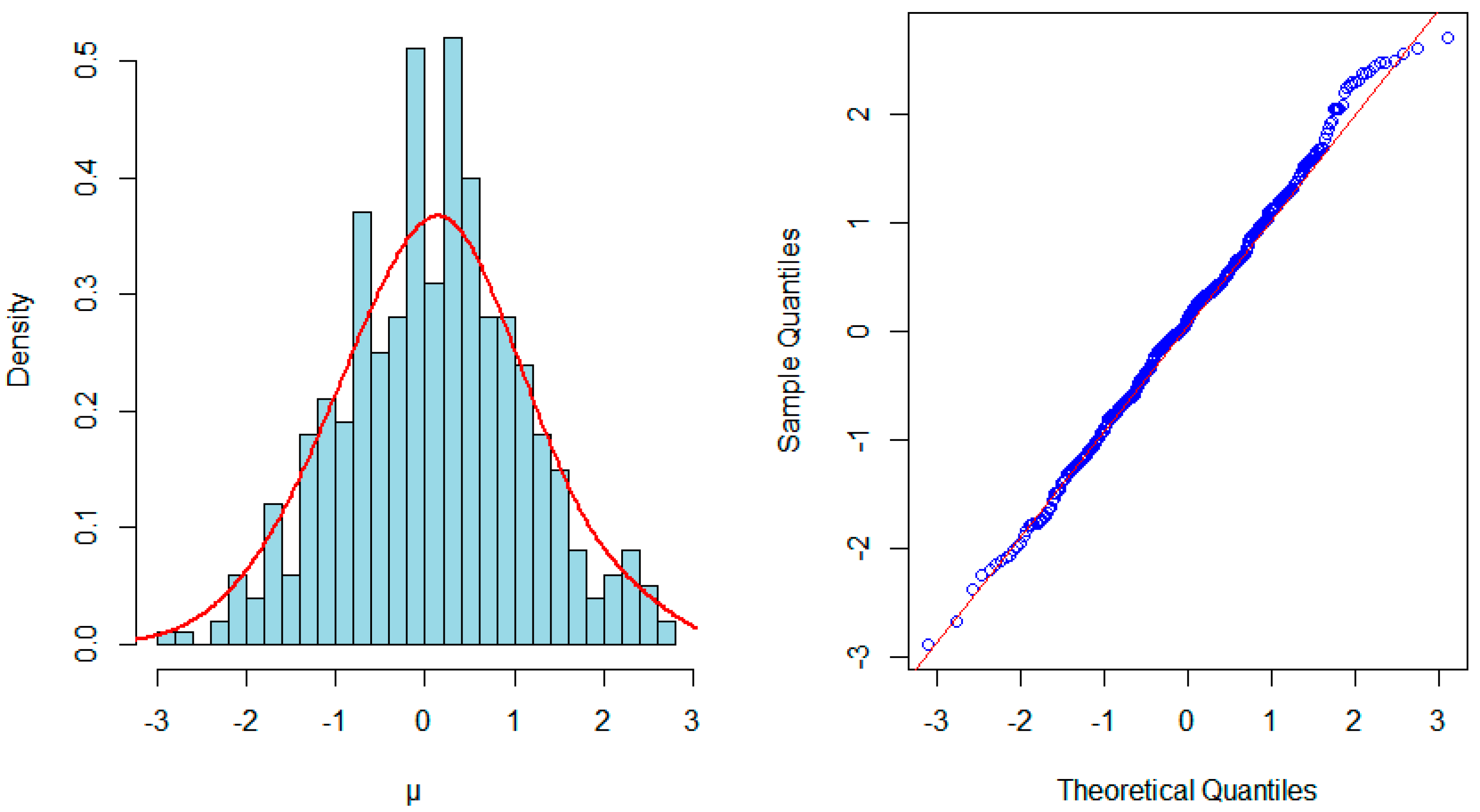
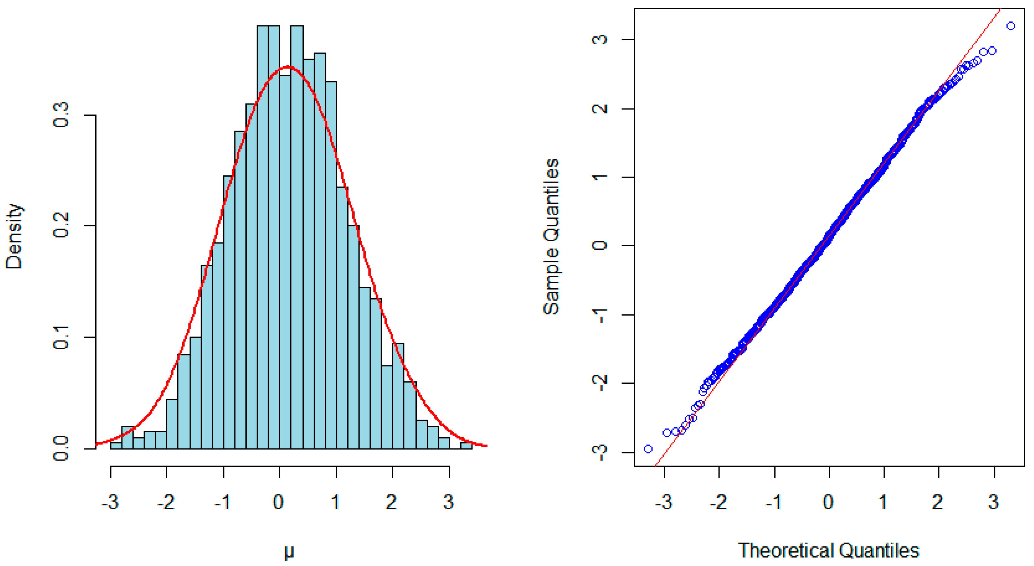
4. Numerical Simulation

In this section, we will carry out a simulation to verify the asymptotic normality of the M-estimator in a linear regression model with AANA errors.

An AANA sequence is given as follows:

$$\mathrm{sequence} 1: e_i={\left(1+a_i^2\right)}^{-1/2}\left({\eta }_i+a_i{\eta }_{i+1}\right), 1\le i\le n,$$

where ${\eta }_1,{\eta }_2,\dots$ are $i.i.d.$ $N\left(0,1\right)$ random variables and $a_i=1/i^2$. The sequence is an AANA sequence but not an NA sequence (see [1]).

We will simulate a regression model:

$$Y_i=x_i{\beta }_0+e_i,$$

(30)

where $x_i=\sin \left(5i\right)+3u_i, 1\le i\le n,$ $i=1,2,\dots ,n,$ $u_i$ is a standard uniform distribution $U\left(0,1\right)$, and the random errors are given by sequence 1.

A derivative function $\Psi (\cdot )$ of function $\rho (\cdot )$ is given by:

$$\Psi \left(x\right)=\{\begin{array}{ll}{\left(1-{\left(x/6\right)}^2\right)}^2,& 1-{\left(x/6\right)}^2>0, \\ 0,& 1-{\left(x/6\right)}^2\le 0\end{array}$$

(see [27]). The sample sizes $n$ are taken as $n=100$, $500$, $1000$, and $2000$, respectively. We use R software to compute $\lambda {\sum }^{-1/2}{L}_n^{1/2}\left({\widehat{\beta }}_n-{\beta }_0\right)$ 1000 times and present the histograms and Quantile–Quantile plots of it in Figure 1, Figure 2, Figure 3 and Figure 4. The red curve in Figure 1 is the kernel density estimate curve, and the red straight line is the reference line whose slope is standard deviation and intercept is mean. The red curves and straight lines in the following figures are also the same meaning.

Figure 1. Histogram and normal Q-Q plot of $\lambda {\sum }^{-1/2}{L}_n^{1/2}\left({\widehat{\beta }}_n-{\beta }_0\right)\stackrel{\wedge}{=}\mu$ with $n=100$.

Figure 2. Histogram and normal Q-Q plot of $\lambda {\sum }^{-1/2}{L}_n^{1/2}\left({\widehat{\beta }}_n-{\beta }_0\right)\stackrel{\wedge}{=}\mu$ with $n=500$.

Figure 3. Histogram and normal Q-Q plot of $\lambda {\sum }^{-1/2}{L}_n^{1/2}\left({\widehat{\beta }}_n-{\beta }_0\right)\stackrel{\wedge}{=}\mu$ with $n=1000$.

Figure 4. Histogram and normal Q-Q plot of $\lambda {\sum }^{-1/2}{L}_n^{1/2}\left({\widehat{\beta }}_n-{\beta }_0\right)\stackrel{\wedge}{=}\mu$ with $n=2000$.

From Figure 1, Figure 2, Figure 3 and Figure 4, we can see that the histograms and Q-Q plots show good fit of the distribution for $\lambda {\sum }^{-1/2}{L}_n^{1/2}\left({\widehat{\beta }}_n-{\beta }_0\right)$ to standard normal distribution as $n$ increases. The simulation results show the asymptotic normality of the M-estimator in the linear regression model with AANA errors.

5. Conclusions

In this article, we mainly study the asymptotic properties of the estimators in the model (1). Many scholars have obtained the asymptotic properties of the estimators in linear models whose errors are independent (see [9,25]). However, the errors are not independent in many applications. In this paper, we suppose that the errors are AANA random variables, which include independent and NA random variables as special cases. The asymptotic normality of M-estimators for the unknown parameters is investigated under some suitable conditions, and the central limit theorem for AANA sequences of random variables is also derived. The results extend the corresponding ones of independent and NA random variables (see [19]). In addition, for model (1), a simulation is carried out to investigate the numerical performance. The aim of our work was to construct general mixing conditions under the classical setting. Although it might be interesting future work, we do not address sequences that have long-range dependence (see [28,29,30]) herein, where the limiting behavior is no longer classical. This is an interesting subject to investigate the limit properties of the estimators in regression models with long-range dependence errors in future studies.

References

- Chandra, T.K.; Ghosal, S. Extensions of the strong law of number of Marcinkiewicz and Zygmund for dependent variables. Acta Math. Hung. 1996, 71, 327–336. [Google Scholar] [CrossRef]
- Chandra, T.K.; Ghosal, S. The strong law of number for weighted averages under dependence assumptions. J. Theor. Probab. 1996, 19, 797–809. [Google Scholar] [CrossRef]
- Yuan, D.M.; An, J. Rosenthal type inequalities for asymptotically almost negatively associated random variables and applications. Sci. China Ser. A 2009, 52, 1887–1904. [Google Scholar] [CrossRef]
- Hu, X.P.; Fang, G.H.; Zhu, D.J. Strong convergence properties for asymptotically almost negatively associated sequence. Discret. Dyn. Nat. Soc. 2012, 2012, 562838. [Google Scholar] [CrossRef]
- Tang, X.F. Some strong laws of large numbers for weighted sums of asymptotically almost negatively associated random variables. J. Inequalities Appl. 2013, 2013, 4. [Google Scholar] [CrossRef]
- Zhang, Y.; Liu, X.S.; Hu, H.C. Weak consistency of M-estimator in linear regression model with asymptotically almost negatively associated errors. Commun. Stat.-Theory Methods 2020, 49, 2800–2816. [Google Scholar] [CrossRef]
- Huber, P.J. Robust estimation of a location parameter. Ann. Math. Statist. 1964, 35, 73–101. [Google Scholar] [CrossRef]
- Huber, P.J. Robust regression: Asymptotics, conjectures and Monte Carlo. Ann. Stat. 1973, 1, 799–821. [Google Scholar] [CrossRef]
- Chen, X.R.; Zhao, L.C. M-Methods in Linear Models; Shanghai Scientific and Technical Publishers: Shanghai, China, 1996. [Google Scholar]
- Huber, P.J.; Ronchetti, E.M. Robust Statistics, 2nd ed.; John Wiley & Sons: New Jersey, NJ, USA, 2009. [Google Scholar]
- Hu, H.C.; Zhang, Y.; Pan, X. Asymptotic normality of DHD estimators in a partially linear model. Stat. Pap. 2016, 57, 567–587. [Google Scholar] [CrossRef]
- Goryainov, A.V.; Goryainov, V.B. M-estimates of autoregression with random coefficients. Autom. Remote Control 2018, 79, 1409–1421. [Google Scholar] [CrossRef]
- Linke, Y.Y.; Sakhanenko, A.I. Conditions of asymptotic normality of one-step M-estimators. J. Math. Sci. 2018, 230, 95–111. [Google Scholar] [CrossRef]
- Wu, Q.Y. Strong consistency of M estimator in linear model for negatively associated samples. J. Syst. Sci. Complex. 2006, 19, 592–600. [Google Scholar] [CrossRef]
- Fan, J. Moderate deviations for M-estimators in linear model with-mixing errors. Acta Math. Sin. 2012, 28, 1275–1294. [Google Scholar] [CrossRef]
- Cui, H.J.; He, X.M.; Kai, W.N. M-estimation for linear models with spatially-correlated errors. Stat. Probab. Lett. 2004, 66, 383–393. [Google Scholar] [CrossRef]
- Muhammad, S.; Sohail, C.; Babar, I. On Some new ridge M-estimators for linear regression models under various error distributions. Pak. J. Stat. 2021, 37, 369–391. [Google Scholar]
- Muhammad, S.; Sohail, C.; Muhammad, A. New quantile based ridge M-estimator for linear regression models with multicollinearity and outliers. Commun. Stat. Simul. Comput. 2023, 52, 1418–1435. [Google Scholar]
- Su, C.; Chi, X. Some results on CLT for nonstationary NA sequences. Acta Math. Appl. Sin. 1998, 21, 9–21. [Google Scholar]
- Butzer, P.L.; Hahn, L. General theorems on rates of convergence in distribution of random variables. 1: General Limit Theorem. J. Multivar. Anal. 1978, 8, 181–201. [Google Scholar] [CrossRef]
- Yuan, D.M.; An, J. Laws of large numbers for Ces’aro alpha-integrable random variables under dependence condition AANA or AQSI. Acta Math. Sin. 2012, 28, 1103–1118. [Google Scholar] [CrossRef]
- Zhang, L.X. A functional central limit theorem for asymptotically negatively dependent random fields. Acta. Math. Hung. 2000, 86, 237–259. [Google Scholar] [CrossRef]
- Ledoux, M.; Talagrand, M. Probability in Banach Space; Springer: Berlin, Germany, 1991. [Google Scholar]
- Petrov, V.V. Limit Theorem for the Sum of Independent Random Variables; Science Publishers: Beijing, China, 1987. [Google Scholar]
- Rao, C.R.; Zhao, L.C. Approximation to the distribution of M-estimates in linear models by randomly weighted bootstrap. Sankhy Ser. A 1992, 54, 323–331. [Google Scholar]
- Anderson, P.K.; Gill, R.D. Cox’s regression model for counting processes: A large sample study. Ann. Stat. 1982, 15, 1100–1120. [Google Scholar] [CrossRef]
- Huber, P.J. Finite sample breakdown of M-and P-estimators. Ann. Stat. 1984, 12, 119–126. [Google Scholar] [CrossRef]
- Düker, M.C. Limit theorems in the context of multivariate long-range dependence. Stoch. Process. Appl. 2020, 130, 5394–5425. [Google Scholar] [CrossRef]
- Kouritzin, M.A.; Sounak, P. On almost sure limit theorems for heavy-tailed products of long-range dependent linear processes. Stoch. Process. Appl. 2022, 152, 208–232. [Google Scholar]
- Bai, S.Y.; Taqqu, M.S. Multivariate limit theorems in the context of long range dependence. J. Time Ser. Anal. 2013, 34, 717–743. [Google Scholar] [CrossRef]
Disclaimer/Publisher’s Note: The statements, opinions and data contained in all publications are solely those of the individual author(s) and contributor(s) and not of MDPI and/or the editor(s). MDPI and/or the editor(s) disclaim responsibility for any injury to people or property resulting from any ideas, methods, instructions or products referred to in the content. |
© 2023 by the author. Licensee MDPI, Basel, Switzerland. This article is an open access article distributed under the terms and conditions of the Creative Commons Attribution (CC BY) license (https://creativecommons.org/licenses/by/4.0/).