Benchmarking Maintenance Practices for Allocating Features Affecting Hydraulic System Maintenance: A West-Balkan Perspective

Abstract

As a consequence of the application advanced maintenance practices, the theoretical probability of failures occurring is relatively low. However, observations of low levels of market intelligence and maintenance management have been reported. This comprehensive study investigates the determinants of maintenance practices in companies utilising hydraulic machinery, drawing on empirical evidence from a longitudinal questionnaire-based survey across the West-Balkan countries. This research identifies critical predictors of technical and sustainable maintenance performance metrics by employing the CA-AHC (Correspondence Analysis with Agglomerative Hierarchical Clustering) method combined with non-parametric machine learning models. Key findings highlight the significant roles of the number of maintenance personnel employed; equipment size, determined on the basis of nominal power consumption; machinery age; and maintenance activities associated with fluid cleanliness in influencing hydraulic machine maintenance outcomes. These insights challenge current perceptions and introduce novel considerations with respect to aspects such as equipment size, maintenance skills and activities with the aim of preserving peak performance. However, the study acknowledges the variability resulting from differing operational conditions, and calls for further research for broader validation. As large-scale heterogeneous datasets are becoming mainstream, this research underscores the importance of using multidimensional data analysis techniques to better understand operational outcomes.

1. Introduction

Nowadays, companies regard maintenance functions as a strategic move for gaining a competitive advantage [1]. The rise of AI (Artificial Intelligence) and ML (Machine Learning) tools provides a “bright avenue” for the growth of Predictive Maintenance (PdM) [2,3]. However, data-driven and sustainable PdM practices face serious difficulties [4], mainly because most systems still rely on RAM (Reliability, Availability and Maintainability) [5] metrics. Additionally, many believe that adopting PdM will significantly reduce downtime [6], improve production flows, and enhance performance [7], ultimately resulting in a failure to fulfil these expectations [8]. Such issues can largely be attributed to problems regarding maintenance strategy selection [9], implementation suitability [10], industrial environment [11], asset management risks [12], and other technological and organisational issues, leading to poor decision making.

Moreover, the availability, as an integral part of OEE (Overall Equipment Effectiveness) [13], with MTBF (Mean Time Between Failure) and MTTR (Mean Time To Repair) as core parameters, is usually perceived as, if not necessarily being, the most critical Maintenance Performance Indicator (MPI) [14]. There are a myriad of factors affecting availability metrics; however, most of them strongly depend on the knowledge and skills of maintainers [15], the efficacy of decision making [16,17], the alignment of maintenance practice with organisational policies, the use of advanced techniques in the diagnosis and prognosis of machines [18,19], reliability modelling and optimisation capabilities [20], the quality of maintenance activities [21], and many other aspects. These multiple interrelated issues are primarily addressed as a single entity on a unit, system or company level. Thus, there is a lack of studies comparing MPIs across different industrial domains. The research (case) studies usually encompass smaller companies, with no evidence concerning their large-scale application. Moreover, existing studies usually do not include qualitative data (e.g., lubrication, monitoring), since such information is hard to synthesise, process and maintain over time. This is primarily the case in asset-intensive industries with heavy-duty machinery, such as hydraulic power systems, where maintenance research is concerned mainly with diagnostic and prognostic aspects [22], thus needing more evidence regarding the impact of latent factors on MPIs. (Note: See Abbreviation)

Nevertheless, entering the digitalisation and cloud-computing era, many companies have started to rely on Big Data and Visual Analytics [23] to assess business issues by utilising large-scale multivariate data analysis (MDA) [24]. MDA’s benefits include its ability to incorporate large-scale heterogenous data—unstructured text, categorical data, numerical data, logs, binary data—and project it in a lower-dimensional subspace, which is necessary to be able to investigate the latent indicators [25] impacting operational performance. Although it has been little engaged with respect to maintenance management, visual analytics utilising MDA is being used to map the landscape of other fields, such as business management, disaster management, and many others [26,27]. As such, in this study, MDA is used to allocate features impacting MPIs via a questionnaire-based survey considering companies utilising hydraulic machinery (Figure 1). The survey included closed- and open-ended questions in order to extract the features impacting MPIs. To achieve this, we conducted a Systematic Literature Review (SLR) to extract the items needed for the survey based on the proposed Research Questions (RQs).

The first research question—RQ1: “What are the most commonly used maintenance performance metrics and/or indicators?”—is used to extract relevant maintenance performance indicators (MPIs) that will be used to build the survey items. The second research question—RQ2: “What are the existing applied maintenance activities under hydraulic systems maintenance practice?”—is designed to extract relevant information regarding the applied maintenance activities, condition monitoring practices, and tools for managing hydraulic machinery. Next, using both open-ended and closed-ended survey questions, since most companies do not have fully implemented CMMSs (Computerised Maintenance Management Systems), it is expected that the responses will include multidimensional data (e.g., text, categorical, numerical). To address these high-dimensional datasets, various dimensionality-reduction techniques must be used to obtain the feature subspace. Finally, the reduced feature subspace is projected against MPIs to allocate the essential features using ML regression algorithms.

The rest of the study is structured as follows. The methodology describes the survey design, including the SLR, the development of the survey items and survey questions, raw data extraction, data wrangling and the ML regression algorithms used to allocate the most critical features impacting the MPIs. The evidence from the longitudinal study, carried out over three years, helped us to gain insights into potential relationships between the MPs (Maintenance Practices) applied and the output results. The third chapter presents the results of the MDA and the extrapolated feature subspace through CA-AHC (Correspondence Analysis with Agglomerative Hierarchical Clustering). Using CA-AHC, we generated components by combining MPs with their associated CFTs (Component Failure Types) and RCFs (Root Causes of Failure) in order to benchmark the MPs. Based on the obtained results, the fourth chapter includes a discussion and analysis of ML post hoc analysis in which features extracted using ML techniques are considered. Finally, the study recapitulates the evidence and provides concluding remarks, describing the implications of this study as well as future research directions.

2. Methodology

2.1. Systematic Literature Review for Extraction of Relevant Performance Indicators

Following the PRISMA (Preferred Reporting Items for Systematic Review and Meta-Analysis) guidelines, we conducted a Systematic Literature Review (SLR) to prepare the items needed to construct the survey. Namely, since we are interested in gathering factors, metrics and/or indicators for measuring the performance of hydraulic machine maintenance, we used the eligibility criteria in

Table 1. Inclusion & Exclusion (I&E) criterias.

I/E Criteria	Subcriteria	Description of Criteria
Inclusion	Time Frame (TF)	Time frame search includes all published articles up to 31 December 2018.
	Full-Text Paper (FTP)	Published editorials, abstracts, presentations, will not be included.
	English Language (EL)	All published articles must be published in English language.
Exclusion	Non-Related (NR)	Articles that are not research studies (e.g., procedures, forewords).
	Loosely Related (LR)	Articles that are not associated with MPIs.
	Partially Related (PR)	Articles that deal with MPIs but lack primer or case study.

. Based on the eligibility criteria, the search strategy and the obtained search results are given in

Table 2. Results based on the search strings.

Search Strings and Criteria	SD	SCOPUS	WOS	Results
“maintenance performance metrics”	41	225	20	119
“maintenance performance indicators”	46	71	2	286
“time between failure” AND “time to repair” AND “hydraulic system”	13	4	0	17
Removing duplicate studies				−53
Removing articles based on the inclusion criteria				−162
Removing articles based on the exclusion criteria				−157
Unavailable articles and those without institutional access				−23
Total articles				27

. In the following, we briefly describe the SLR and the indicators extracted and used to build the survey items (Figure 2).

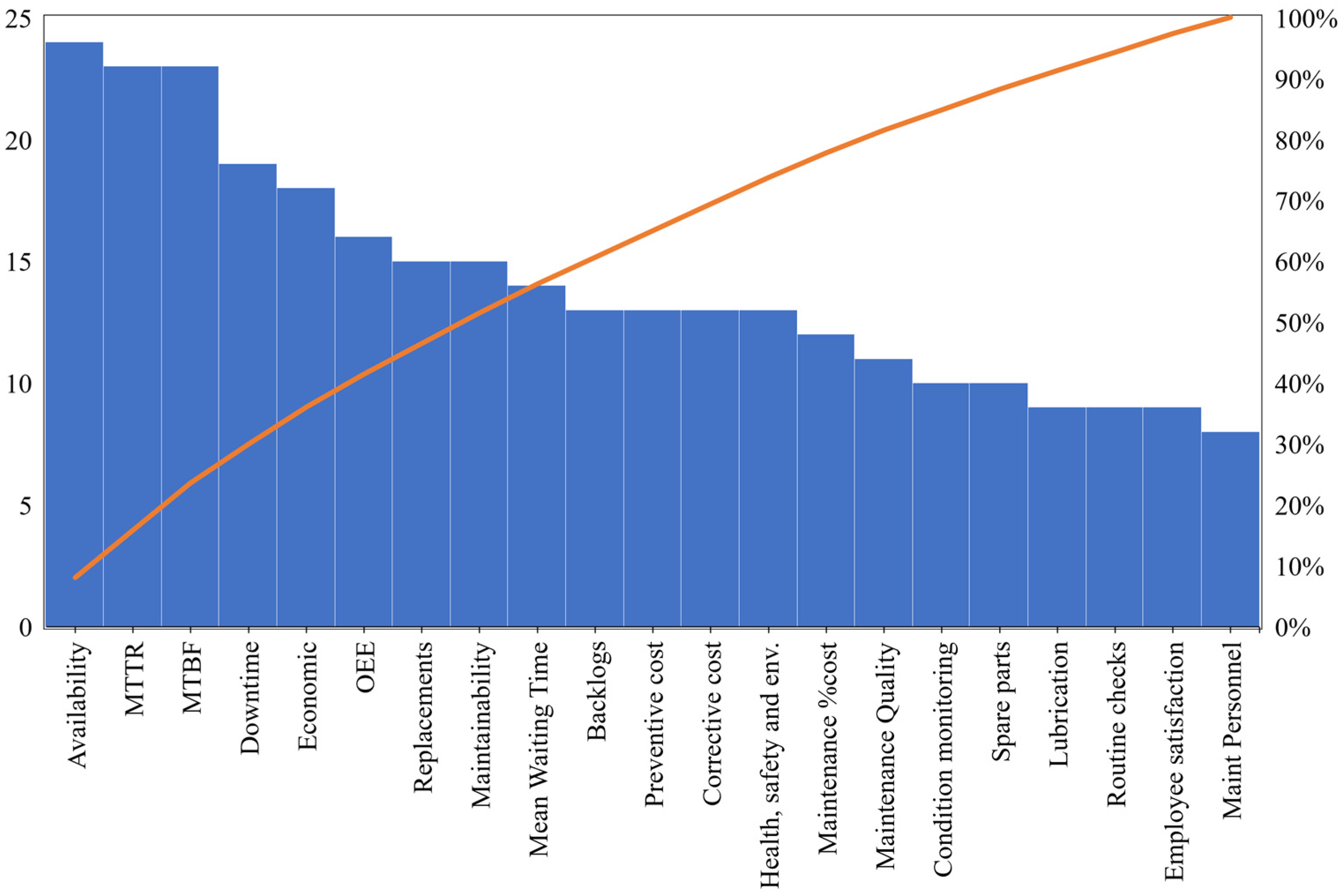
After finishing the SLR, the final sample included 27 articles. Based on the retrieved articles, almost all articles, without exception, highlighted Availability, MTTR, and MTBF as the three most essential MPIs (Figure 2). However, MTTR and MTBF are parameters that need to be input in order to derive Availability estimates.

Earlier work [28,29] was mostly dedicated to allocating and benchmarking MPIs using different types of frameworks [30], and was performed by Parida, A. et al. [29,31,32], Kumar, U. et al. [33], and Van Horenbeek and Pintelon, L. [34,35]. Most frameworks are designed as secondary data on the basis of an overview [36] with multicriteria decision-making tools [37] such as AHP (Analytical Hierarchy Process) [38], ANP (Analytical Network Process) [39,40], and ELECTRE [41]. Considering the practical application of the use of MPIs, most of the work is being formed in the context of industrial manufacturing [42,43,44,45,46], business organisations [47], specific production case studies [48], or even in healthcare [49]. Thus, since there is still an ongoing debate regarding framework appropriateness and maintenance practice suitability [50,51] in different types of industry, most of the research still emphasises the availability metric of the maintenance function, since it is an integral part of the OEE (Overall Equipment Effectiveness) [52,53]. Although most of the indicators are concerned with economic and technical evaluation metrics, due to recent environmental concerns, many are incorporating sustainability indicators [53,54] as maintenance indicators.

The recent work on MPIs utilises a broad range of MPIs and performance metrics (Figure 3), presumably due to the computational ability of machine learning techniques that can translate large-scale heterogenous datasets into a low-dimensional feature space. On the basis of the SLR, we used the performance metrics and the performance of associated maintenance activities to derive the information we required to reach a consensus regarding the relationship between maintenance and operation activities and performance. Next, since in the SLR we did not find evidence of addressing specific types of failure or root causes of failure and their overall impact on maintenance performance; we decided to include these output metrics. Finally, as recent work has started utilising sustainability metrics, we also included lubricant waste as one of the essential output metrics regarding the operational performance of hydraulic machinery.

2.2. Study Design and Data Wrangling

The study design consists of three parts: (1) survey design; (2) survey raw data processing and data wrangling; and (3) feature subspace extraction and data analysis (Figure 4). The survey design consists of the SLR-based extraction of MPIs (Figure 4a); the survey realisation workflow (Figure 4b); the geographical representation of the survey results (Figure 4c); company characteristics (Figure 4d); strategic and operational level of maintenance activities (Figure 4e); maintenance performance metrics and indicators extracted (Figure 4f); CA considering feature subspace (Figure 4g); AHC clustering (Figure 4h); extraction of features by importance using ML (Machine Learning) algorithms considering output MPIs (Figure 4i). The survey design was performed over the course of several iterations with respect to organisational, maintenance management and performance structures and characteristics. After the survey had been adjusted and was deemed suitable, the CA and Agglomerative Hierarchical Clustering (AHC) models were used to generate a feature subspace based on the extracted raw data. By using MPs and failure-associated characteristics, clusters were created, which were then used to allocate features in consideration of output maintenance metrics. Finally, selected clusters were subjected to output metrics to isolate the features, including maintenance programs, factors and activities via ML algorithms.

2.3. Survey Design and Realisation

The design of survey items (Figure 5) started with an SLR (Task 1) regarding keywords and search strings (Table 2). After the SLR, the authors individually synthesised papers (Task 2) based on the eligibility criteria. The extraction of MPIs to be included in the survey was performed on the basis of interrater agreement using Cohens’ K > 0.7 (K = 0.89). The final list included 33 indicators that satisfied the criterion (Task 3). However, in the preliminary draft of the survey targeting companies utilising hydraulic applications in the West Balkan Peninsula, several MPIs were removed (Task 4). This is primarily because different types of maintenance policy and databases had different MPIs, most of which were unavailable for disclosure to the public (e.g., maintenance costs) or were not recored (e.g., injuries, backlogs). The first draft contained 77 survey questions. Next, consultations were carried out with academic experts in the field (Task 5), who considered some survey questions to be redundant, and could be merged or split into subquestions. In addition, other survey questions were deemed irrelevant, such as those covering stoppages that were consequences of non-hydraulic failure events (e.g., structural failures, mechanical failures, electrical failures). This resulted in the elimination of several unrelated questions, merging some and splitting others into subquestions (Task 6). The first version of the survey was sent to the sample of 5 companies as a mini (pilot) survey study in order to gather information and insights regarding the understandability, completeness, reliability, and validity of the open- and closed-ended items of the questionnaire (Task 7).

After administrating the survey to the companies, minimicking the conditions of the target group companies that utilise hydraulic machinery, the results showed that the survey questions regarding the maintenance policies, programs and maintenance activities needed to be clarified. Namely, 4/5 companies still required specifically designed and recorded maintenance policies rather than maintenance procedures in the context of a quality management system. Hence, we reformulated questions regarding maintenance policies into questions about maintenance practices, since some practices included several different activities (e.g., time-based, corrective, and opportunity-based activities) within a given procedure. Additionally, some maintenance activities for replacing parts were not recorded in backlogs; thus, output metrics regarding spare parts management, work order logs, replacements, and preventive and corrective costs were removed, and only availability metrics (MTBF, MTTR) were left. Additionally, the provision of datasets regarding the exact energy consumption of each hydraulic machine was eliminated, since none of the companies had measurements of each hydraulic system’s energy consumption. Instead, nominal working pressure and nominal working flows were used as measures for describing the size of the equipment. However, all of the respondents were able to provide information regarding the most common failure causes and root causes of failure. Regarding the MTBF and MTTR metrics, 3/5 companies had a log of failure times in the pilot study. In contrast, others did not have a complete record, which resulted in the formulation datasets for the extraction of failure times using range values (e.g., 100–200 h TBF). From a sustainability perspective, the waste hydraulic fluid data were available for extraction using the survey. None of the questions were found to be offensive.

Furthermore, the feedback from the industrial experts, maintenance managers and engineers on a strategic level (Task 8) resulted in the elimination of survey items mostly on the basis of the time required to complete the survey, the public disclosure of costs and energy consumption data per machine, and the lack of records and procedures for documenting activities via logbooks or data management systems. Additionally, some companies incorporate a centralised top maintenance management level, including a manager or a director. Here, the responsibility falls under the technical department, whether or not its management is the director’s responsibility. Next, as was later confirmed, some companies still employ a maintenance department or section that is responsible for maintaining and keeping records of hydraulic machine failures. In some of these cases, some or all maintenance management, including diagnosis and prognosis, were outsourced. In such instances, data records were requested from the companies to which the tasks were outsourced or from the experts conducting in-house maintenance activities, and they were asked to provide records and fill out the survey. This helped improve the questions related to maintenance diagnosis and prognosis, and the survey options were extended with external experts and outsourced maintenance activities.

After redesigning and preparing the final draft of the survey (Task 9), the surveyed companies and industrial experts agreed that the survey of 22 questions (with 5 sub-questions) included all information necessary for the analysis. Therefore, the first realisation phase started in September 2019 (Task 10) and lasted until May 2021. In the first run, 81 samples, which included most of the companies in Serbia, were collected. Since the sample size was still small, we conducted a longitudinal study. Thus, in the second run (September 2020–June 2021), 100 companies participated. Next, considering that some companies changed their initial practices on the basis of insights derived from their previous state, we thought that data could be biased due to discrepancies between initial and follow-up (second-run) results. Therefore, we decided to include a third and final run, which ultimately led to results being gathered from 115 companies, from which data were synthesised and subjected to analysis. The obtained results proved compelling, complete and valid, since, based on the first (11% missing data) and second run (4% missing data), only 1.3% of data were missing. The missing data were later excluded from the analysis or replaced by the mean average value to reduce the bias/variance tradeoff. The complete survey is presented in Supplementary Material File S1.

2.4. Survey Items and Data Extraction

The survey design (Figure 5) started in February 2019 and lasted until June 2019. The survey questions were segmented into three facets, namely: (i) organisational characteristics; (ii) characteristics of maintenance functions; and (iii) output data as performance metrics. The organisational facet included questions regarding organisational structure and asset characteristics. Organisational and asset characteristics include information regarding the company and its associated hydraulic machinery (e.g., age, type). The maintenance characteristics include the department’s size, the staff and their qualifications, the condition monitoring tools (e.g., sensors, instruments) available, and preventive/corrective activities performed (e.g., filter replacement time, time to complete oil change). The output performance metrics measured include MTBF (Mean Time Between Failures), MTTR (Mean Time To Repair); CFTs (Component Failure Types), RCFs (Root Causes of Failure); and WOMM (Wasted Oil per Machine-Month). A complete list of the survey questions is provided in Appendix A.

2.5. Correspondence Analysis (CA)

Since the survey contains mostly categorical data, contingency tables are formed and χ² distance metrics are used for CA. The contingency table(s) consider I categories (rows) of variable V₁, where i = 1, 2… I, and j categories (columns) of variable V₂, where j = 1, 2…J. The value x_i,j corresponds to the values of a variable with i rows and j columns, with n instances. Using contingency tables, we first calculate the probabilities as follows:

$$f_{ij}=\frac{x_{ij}}{n},$$

(1)

where the sum of rows equals the marginal probability:

$$f_{.j}={\sum }_{i=1}^I{f}_{ij},$$

(2)

and for the sum of columns, the marginal probability:

$$f_{i.}=\sum _{j=1}^J{f}_{ij}.$$

(3)

The relationship between selected variables is measured using the the χ² distance:

$${\chi }_{obs}^2={\sum }_{i=1}^I{\sum }_{j=1}^J\frac{{(n{f}_{ij}-n{f}_{i.}{f}_{.j})}^2}{n{f}_{i.}{f}_{.j}},$$

(4)

where nf_ij is the observed probability and nf_i.f_.j is the theoretical probability, and factoring n out of Equation (4), we get the total inertia Φ²:

$${\chi }_{obs}^2={\sum }_{i=1}^I{\sum }_{j=1}^{J}n\frac{{(f_{ij}-f_{i.}{f}_{.j})}^2}{f_{i.}{f}_{.j}}=n{\Phi }^2.$$

(5)

The CA is described as point clouds, as proposed in [55], alongside mathematical formulations [56,57]. Considering the number of row profiles i, we obtain a cloud of profiles N_I. With the generated point cloud, we add the point G_I, depicting the centre of gravity with coordinate f_.j. G_I can be considered a centre of gravity if we associate each point i with the weight proportional to its marginal value (f_i.). The space then compares profile i with G_I using a measure of distance. As stated, the distance between i and i′ is defined as follows:

$$d_{{\chi }^2}^2\left(i,i^{\prime }\right)={\sum }_{j=1}^J\frac{1}{f_{.j}}{\left(\frac{f_{ij}}{f_{i.}}-\frac{f_{i\prime j}}{f_{i\prime .}}\right)}^2.$$

(6)

Although this could suggest Euclidian distance, the χ² compares the sum of differences, where each dimension J is associated with a weight 1/f_.j. Therefore, the centre of gravity G_I corresponds to the mean profile as follows:

$$d_{{\chi }^2}^2\left(i,G_I\right)={\sum }_{j=1}^J\frac{1}{f_{.j}}{\left(\frac{f_{ij}}{f_{i.}}-f_{.j}\right)}^2.$$

(7)

The same principles are used for estimating the distances in the column profile. A column profile is a set of I values in ℝ^I dimensional space. The coordinates of the jth point are f_ij/f_.j, and all of the j points together form the N_j cloud. The central point, i.e., the centre of gravity G_J, is added to the coordinate f_i. in the Ith dimension. G_I is the centre of gravity as long as we assign a column profile j a weight corresponding to its marginal probability f_.j. Next, we estimate the distances d between points j and j′ using the χ² distance metric as follows:

$$d_{{\chi }^2}^2\left(j,j^{\prime }\right)={\sum }_{i=1}^I\frac{1}{f_{i.}}{\left(\frac{f_{ij}}{f_{.j}}-\frac{f_{ij\prime }}{f_{.j\prime }}\right)}^2,$$

(8)

and the centre of gravity G_J is estimated as follows:

$$d_{{\chi }^2}^2\left(j,G_J\right)={\sum }_{i=1}^I\frac{1}{f_{i.}}{\left(\frac{f_{ij}}{f_{.j}}-f_{i.}\right)}^2.$$

(9)

If independence exists, the conditional probability is equal to the marginal probability for all i (f_.j = f_ij/f_i.), meaning that all profiles are the same as the mean, i.e., N_I becomes G_I. As such, we measure the inertia using Equation (5), as follows:

$$\mathrm{I}\mathrm{n}\mathrm{e}\mathrm{r}\mathrm{t}\mathrm{i}\mathrm{a}\left(\frac{N_I}{G_I}\right)={\sum }_{i=1}^I{\sum }_{j=1}^J\frac{{\left(f_{ij}-f_{i.}{f}_{.j}\right)}^2}{f_{i.}{f}_{.j}}=\frac{{\chi }^2}{n}={\Phi }^2.$$

(10)

The same holds for N_J: Inertia(N_J/G_J) = Inertia(N_I/G_I). Therefore, Φ² represents the strength of the link. The CA proceeds, for all components (i.e., factors), by projecting N_I to axes C1 and C2, forming a plane P. Finding the plane P is determined by the criteria of maximum inertia, such that:

$${\sum }_{i=1}^I{f}_{i.}{\left({OH}_i\right)}^2,$$

(11)

is maximal and is used to determine the M_i point that corresponds to the Ith profile on the plane P, where OH_i represents the distance to the origin G_I = O. The plane P is the sum of the inertia, such that the projected H_i overall i is maximal. The C1 and C2 axes (components) represent maximal inertia such that C2⊥C1, and as a result, we obtain plane P. The inertia λ_s of the sth axis is then:

$${\sum }_{i=1}^I{f}_{i.}{\left({OH}_i^s\right)}^2={\lambda }_s,$$

(12)

and λ_s represents the eigenvalue of the C_s. Calculating f_i. on C_s (the same as for the column) over the total inertia of the λ_s is performed as follows:

$$Contribution\left(f_{i.},{\lambda }_s\right)=\frac{f_{i.}{\left({OH}_i^s\right)}^2}{{\lambda }_s},$$

(13)

where summation leads to the inertia of C_s, and we determine the quality (Qual) of the representation as follows:

$${Qual}_s=\frac{{\sum }_{i=1}^I{f}_{i.}{\left({OH}_i^s\right)}^2}{{\sum }_{i=1}^I{f}_{i.}{\left({OM}_i\right)}^2}=\frac{{\lambda }_s}{{\sum }_{k=1}^K{\lambda }_k},$$

(14)

where OM_i is the distance between the M_i point and the origin O. The numerator represents the inertia of N_I on the axis C_s, and the denominator is the total Inertia(N_I) = Φ². Calculating the position on the plot of rows and columns, we use transitional formulas to determine the coordinates of row i on the sth axis (F_s) as follows:

$$F_s\left(i\right)=\frac{1}{\sqrt{{\lambda }_s}}{\sum }_{j=1}^J\frac{f_{ij}}{f_{i.}}{G}_s(j),$$

(15)

where G_s(j) is the coordinate of the column j on the sth axis, and λ_s is the inertia of the sth axis. Permuting G_s and F_s, we obtain the same outcome for the different barycentre. Intuitively, the number of axes that contain non-zero inertia is S ≤ min(J − 1, I − 1). Estimating the Φ² points of the axes gives us:

$${\Phi }^2={\sum }_{k=1}^{\min (I-1,J-1)}{\lambda }_k\le \min \left(I-1,J-1\right).$$

(16)

2.6. Clustering CA Components Using Agglomerative Hierarchical Clustering (AHC)

Agglomerative Hierarchical Clustering (AHC) is added to replace the inability of CA to project data in more than three dimensions. The two important measures of the AHC are distance and linkage. The AHC assumes that each point x is a singleton [58]. The algorithm creates a collection of higher-level clusters c_i by merging the point(s) (singletons) into a new cluster c_i’. In order to measure the distances between points, the Euclidian distance is used [59]:

$$ED\left(p,q\right)=\sqrt{{\sum }_i^n{(p_i-q_i)}^2}=‖x_c-x_{c^{\prime }}‖,$$

(17)

where p and q are coordinates of c. For the cluster linkage, we use Ward’s method [60]. The method is imputed by the Lance–Williams algorithm [59] and calculated as:

$$d\left({\mathbf{g}}_i,{\mathbf{g}}_j\right)=\frac{\left|i\right|\left|j\right|}{\left|i\right|+\left|j\right|}{‖{\mathbf{g}}_i-{\mathbf{g}}_j‖}^2,$$

(18)

where agglomeration factors are estimated by the Lance–Williams dissimilarity:

$${\alpha }_i=\frac{\left|i\right|+\left|k\right|}{\left|i\right|+\left|j\right|+\left|k\right|};\beta =-\frac{\left|k\right|}{\left|i\right|+\left|j\right|+\left|k\right|};\gamma =0,$$

(19)

such that ǀiǀ represents the number of objects in cluster i, and g represents the centre coordinates estimated as:

$$\mathbf{g}=\frac{\left|i\right|{\mathbf{g}}_i+\left|j\right|{\mathbf{g}}_j}{\left|i\right|+\left|j\right|}.$$

(20)

After obtaining the distance metrics and performing the clustering of principal components, the CA-AHC is performed.

2.7. Machine Learning Algorithms and Evaluation Metrics

The obtained AHC-CA clusters are then subjected to the machine learning regression algorithms, where independent variables consider maintenance performance indicators, specifically MTBF, MTTR and WOMM. Next, algorithm selection is performed by considering algorithms that can handle categorical (e.g., nominal and ordinal) and continuous/numeric (scale and metric) data as predictors. Next, for selecting between parametric and non-parametric ML algorithms, we used the Shapiro–Wilk test (p < 0.05) to test the normality assumption. As it turned out, the normality assumption was violated, and the non-parametric counterpart ML algorithms were selected. The ML algorithms used for the analysis include the SVR (Support Vector Regression) [60], kNN (k-Nearest Neighbour) [61], DT (Decision Tree) [62] and RF (Random Forest) [63] regression algorithms. The reader should not know that although SVR is generally a parametric algorithm, we used an RBF (Radial Basis Function), as it is the most frequently applied Kernel trick in the literature [61].

The evaluation metrics used include the following. The MSE (Mean Squared Error):

$$\mathrm{M}\mathrm{S}\mathrm{E}=\frac{1}{n}{\sum }_{i=1}^n{(y_i-\widehat{y_i})}^2,$$

(21)

as well as the RMSE:

$$\mathrm{R}\mathrm{M}\mathrm{S}\mathrm{E}=\sqrt{\mathrm{M}\mathrm{S}\mathrm{E}}=\sqrt{\frac{1}{n}{\sum }_{i=1}^n{(y_i-\widehat{y_i})}^2}.$$

(22)

and the MAE:

$$\mathrm{M}\mathrm{A}\mathrm{E}=\frac{1}{n}{\sum }_{i=1}^n\left|y_i-\widehat{y_i}\right|.$$

(23)

where y_i is the actual value, $\widehat{y_i}$ is the predicted value, and n is the number of observations. The R² coefficient of determination is calculated as:

$${\mathrm{R}}^2=1-\frac{{MAE}_{model}}{{MAE}_{baseline model}},$$

(24)

which represents the proportion of variance in the dependent variable predicted by independent variables. Finally, the analysis is performed using the open-source software JASP. JASP is built using R packages for DT (rpart), RF (randomForest), SVM (e1071), and kNN (kknn). Under each category, feature importance is established by relative importance and mean decrease in accuracy provided by JASP, from which the results are obtained.

3. Research Results

3.1. Survey Insights and Descriptions

From the sample of 297 companies, 7.41% (22 companies) of respondents strongly underscored that they were unwilling to participate in the study. Then, 19.53% (58 companies) of respondents were willing to participate in the survey, but no results were obtained, even after contacting them three times. Next, 34.3% of respondents (102 companies) did not respond. The final dataset comprises 115 companies (38.72% response rate).

The sample includes large (51.3%), medium (37.4%), and small (11.3%) companies. According to the NACE (Nomenclature of Economic Activities), the respondents consisted of 8.7% AFF (Agriculture, forestry, and fishing), 19.1% CON (Construction), 47.0% MAN (Manufacturing) and 25.2% M&Q (Mining and Quarrying) companies. Considering these asset characteristics, the average distribution of HMA (Hydraulic Machinery Age) across classes is presented in

Table 3. Descriptive statistics of survey results.

Feature	AFF 1	CON 1	MAN 1	M&Q 1
HMA	10.5	10.25	11.80	10.54
NoM	62.4	41.86	52.94	85.2
MPPM	0.55	0.37	1.09	0.62

AFF ¹ = agriculture, forestry, and fishing; CON ¹ = construction; MAN ¹ = manufacturing; M&Q ¹ = mining and quarrying.

. The NoM (Number of Machines) was the greatest in M&Q. The MPPM (Maintenance Personnel per Machine) was the highest in MAN (0.75), and the lowest in CON (0.45).

The CFT (Component Failure Type) item is used to construct categories based on text mining. Therefore, the most frequently reported failures include “hoses OR pipes”, 85.65%; pumps, 71.3%; “actuators OR cylinders” OR “linear OR rotary”, 53.05%; sensors, 23.48%; “servo OR proportional”, 21.6%; “pressure OR flow OR check OR regulation valves”, 4.35%; accumulators, 3.48%; “ice OR internal combustion engine” OR “em OR electrical motor”, 3.48%; and other, 3.4%. These categories are divided into ten categories for the analysis. In terms of RCFs (Root Causes of Failure), the most-reported RCFs were those related to seals (92.2%), leakage (64.35%), overload (42.61%), temperature (24.35%), technician and operator mistakes (23.48%), air and water contamination (10.43%), “wear OR fatigue” (4.35%), particle contamination (3.48%), and other stoppages (27.83%).

It should be noted that most companies do not use a single MP, but rather a combination of different MPs, and for the sake of understanding, we use curly brackets to report cases in which companies utilise MP variants. For instance, in cases where a company itilises OM, CBM and PdM practices, this will be noted as “{OM. CBM. PdM.}”. Finally, the CA-AHC analysis is performed in MINITAB v17.0.

3.2. Relationship between MPs and CFTs Using CA-AHC

The obtained results show that the total inertia is Φ² = 1.435, with the first two components accounting for 50% of the total inertia (

Table 4. Quality of interpretation using MPs and CFTs.

Dimension	SV	Inertia	χ2	Sig.	Proportion of Inertia		Confidence SV
					Accounted	Cumulative	St. dev	Corr. C2	Corr. C3
C1	0.673	0.452			0.315	0.315	0.051	0.159	0.417
C2	0.526	0.277			0.193	0.508	0.083		0.160
C3	0.515	0.265			0.185	0.693	0.099
C4	0.406	0.165			0.115	0.808
C5	0.355	0.126			0.088	0.896
C6	0.267	0.071			0.050	0.946
C7	0.187	0.035			0.024	0.970
C8	0.156	0.024			0.017	0.987
C9	0.130	0.017			0.012	0.999
C10	0.040	0.002			0.001	1.000
Total		1.435	165.021	0.000	1.000	1.000

). Among the mentioned MPs, {OM} and {PM. CBM. PdM.} alone account for >0.95 of the quality (

Table 5. Overview of row components of MPs and CFTs.

MP	Mass	Coordinates			λ	Correlation			Contribution
		C1	C2	C3		C1	C2	C3	C1	C2	C3	Qual
CBM	0.113	−0.915	0.288	0.338	0.160	0.209	0.034	0.049	0.591	0.058	0.081	0.731
FBM	0.096	0.055	−0.508	−0.021	0.105	0.001	0.089	0.000	0.003	0.234	0.000	0.238
FBM. PM.	0.104	−0.885	0.012	0.143	0.160	0.181	0.000	0.008	0.510	0.000	0.013	0.523
FBM. PM. CBM.	0.096	0.259	−0.760	−0.319	0.114	0.014	0.200	0.037	0.056	0.483	0.085	0.624
FBM. PM. OM.	0.061	−0.339	0.208	−0.324	0.044	0.015	0.009	0.024	0.158	0.059	0.145	0.362
OM	0.035	10.861	0.382	20.115	0.290	0.266	0.018	0.586	0.415	0.018	0.536	0.969
PdM	0.026	0.321	0.224	−0.964	0.050	0.006	0.005	0.091	0.054	0.026	0.488	0.568
PM	0.330	−0.031	0.022	0.075	0.061	0.001	0.001	0.007	0.005	0.003	0.031	0.038
PM. CBM.	0.052	1.092	−1.023	−0.343	0.175	0.138	0.197	0.023	0.356	0.313	0.035	0.704
PM. CBM. PdM.	0.078	0.945	10.246	−0.760	0.244	0.155	0.439	0.170	0.286	0.497	0.185	0.968
PM. DM.	0.009	−0.869	0.489	0.360	0.031	0.015	0.008	0.004	0.210	0.066	0.036	0.312
Total	1.000				1.435	1.000	1.000	1.000

). On the other hand, it can be seen that {PdM} accounts for significantly less of the inertia λ_PdM = 0.05; however, with the three proposed axes, the Qual_{PdM} = 0.568, showing high interpretability.

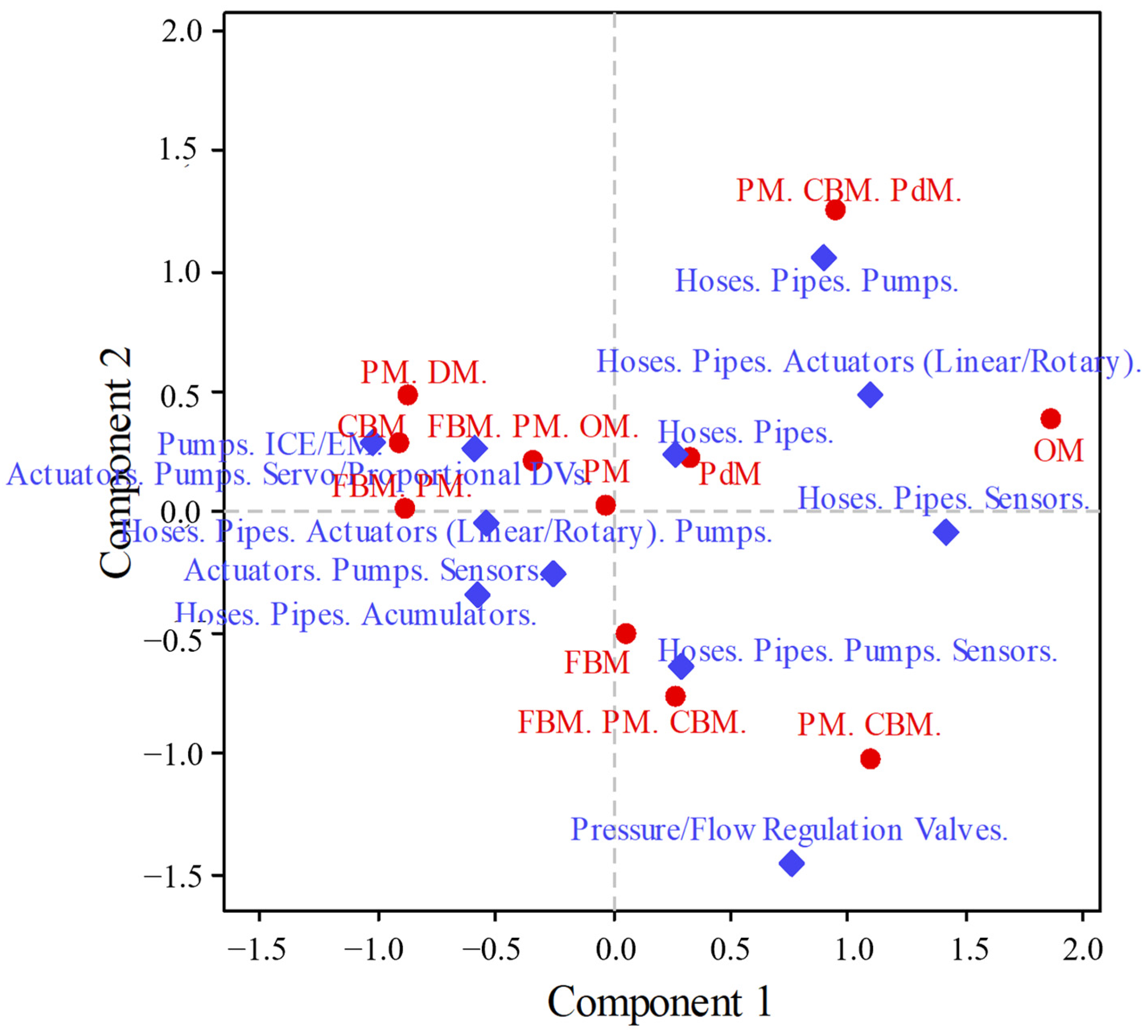
Considering the association between MPs and the components of CA, the data suggest that {CBM} and {OM} are correlated with C1, while {FBM. PM. CBM.}, {PM. CBM.}, and {PM. CBM. PdM.} are correlated with C2. When considering the third component, C3, of CA, it can be observed that only {OM} has a higher tendency to associate with this component, suggesting that {OM} differs significantly, i.e., that it has a higher inertia from the centre of the CA. Conversely, {PM}, as the most common MP applied, does not seem to correlate with other components of CA, which is why it is positioned as the centre of gravity on the CA biplot.

In CA analysis (Figure 6), interpreting and making conclusions solely on the basis of the biplot can be insufficient. For instance, the points on the left ({PM. DM.}; {CBM}; {FBM. PM. OM.}; {FBM. PM.}) cluster, while same can be said for ({FBM}; {FBM.PM.CBM.}; {PM. CBM.}). However, looking at the points, it cannot be confirmed that {FBM} and {PM. CBM.} cluster, even when their similarity might suggest an association between the two. Looking at {PM. CBM.} and {PM. CBM. PdM.}, the results imply no association between the two. However, interpreting the results in Table 4, coordinates of C1_{{PM. CBM.};coord} = 1.092 and C3_{{PM. CBM.};coord} = −0.343 are closely associated with C1_{{PM. CBM. PdM.};coord} = 0.945 and C3_{{PM. CBM. PdM.};coord} = −0.760.

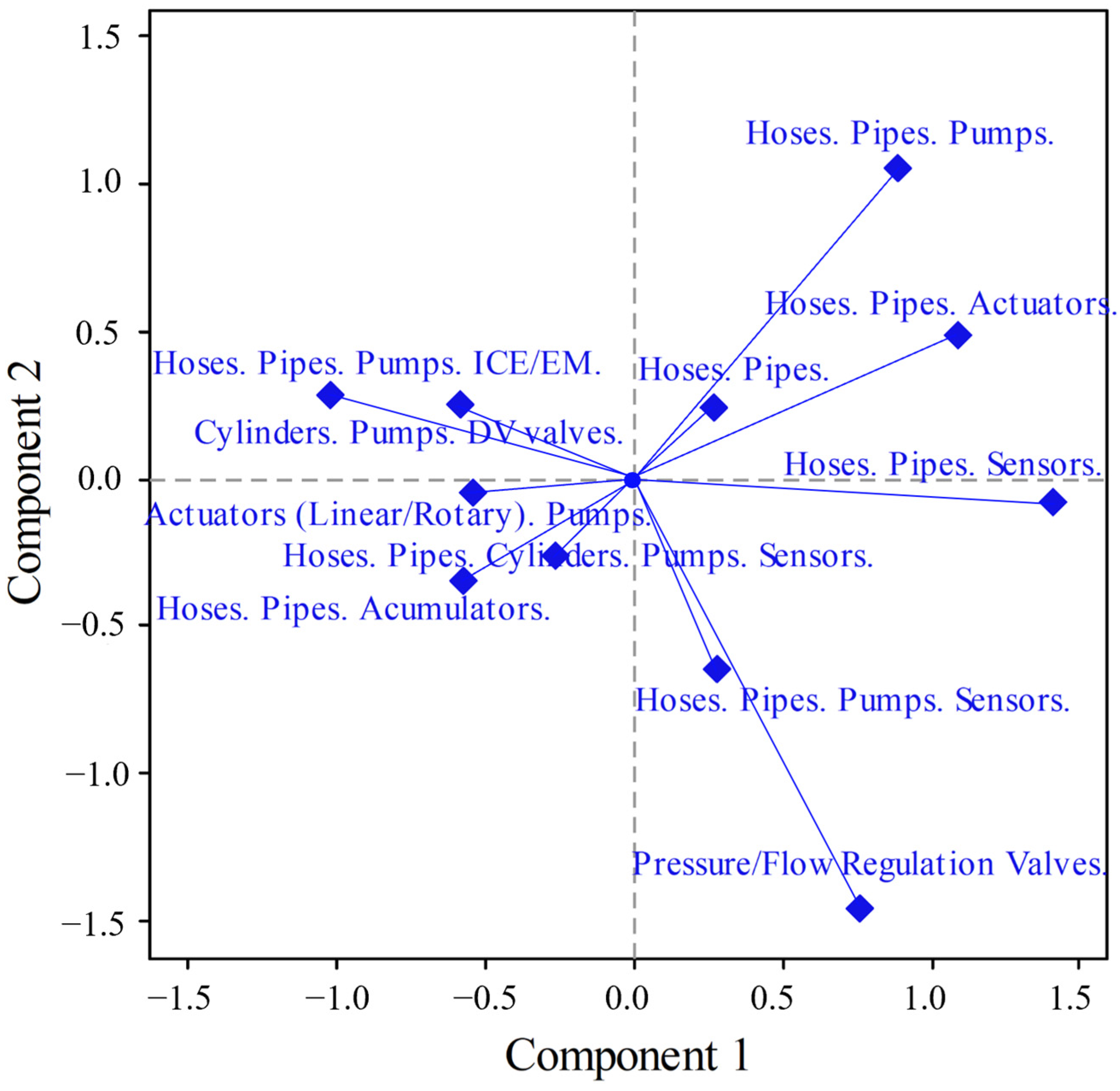
Observing the column profiles, the results show that {Hoses. Pipes. Pumps.}, λ_HPP = 0.236, followed by {Hoses. Pipes. Sensors.}, λ_HPS = 0.211, and {Pressure. Flow. Contr.-Regulation. Valves}, λ_PFCR = 0.181, account for most of the explained inertia. However, {Hoses. Pipes. Actuators.} are indicated to have higher quality Qual_HPA = 0.851 > Qual_PFCR = 0.686.

Looking at the left side of C1 (Figure 7), there is a discrepancy between the frequency and variety of failures, while on the right side of the C1-axis (positive), there is an increase in the number of sensor failures. This is a valuable insight for detecting associations with MPs and for better interpretation of the biplot.

Although CA (Figure 8) provides different ways of interpreting the association between categories, post hoc analysis can be misleading if the quality of the visualisations is neglected. Looking at the row profile (Table 5) and column profile (

Table 6. Overview of column components of MP and CFT.

CFT	Mass	C1	C2	C3	λ	Correlation			Contribution
						C1	C2	C3	C1	C2	C3	Qual
Hoses. Pipes.	0.096	0.269	0.239	−0.236	0.079	0.015	0.020	0.020	0.088	0.069	0.068	0.225
Hoses. Pipes. Actuators.	0.070	1.090	0.483	0.611	0.147	0.183	0.059	0.098	0.563	0.111	0.177	0.851
Hoses. Pipes. Actuators. Pumps.	0.200	−0.537	−0.052	−0.024	0.104	0.127	0.002	0.000	0.556	0.005	0.001	0.562
Hoses. Pipes. Accumulators.	0.035	−0.573	−0.340	0.021	0.078	0.025	0.015	0.000	0.147	0.052	0.000	0.199
Hoses. Pipes. Act. Pumps. S-PV.	0.217	−0.585	0.257	0.185	0.130	0.164	0.052	0.028	0.569	0.110	0.057	0.737
Hoses. Pipes. Act. Pumps. Sensors.	0.043	−0.258	−0.260	0.174	0.066	0.006	0.011	0.005	0.044	0.045	0.020	0.109
Hoses. Pipes. Pumps.	0.070	0.897	1.05	−1.12	0.236	0.124	0.277	0.326	0.237	0.324	0.366	0.927
Hoses. Pipes. Pumps. ICE/EM.	0.035	−1.02	0.289	0.435	0.070	0.080	0.011	0.025	0.521	0.042	0.094	0.657
Hoses. Pipes. Pumps. Sensors.	0.148	0.289	−0.645	−0.350	0.134	0.027	0.222	0.068	0.092	0.458	0.135	0.684
Hoses. Pipes. Sensors.	0.043	1.414	−0.081	1.57	0.211	0.192	0.001	0.402	0.412	0.001	0.506	0.920
Pressure/Flow Control-Reg.	0.043	0.759	−1.45	−0.406	0.181	0.055	0.332	0.027	0.139	0.508	0.040	0.686
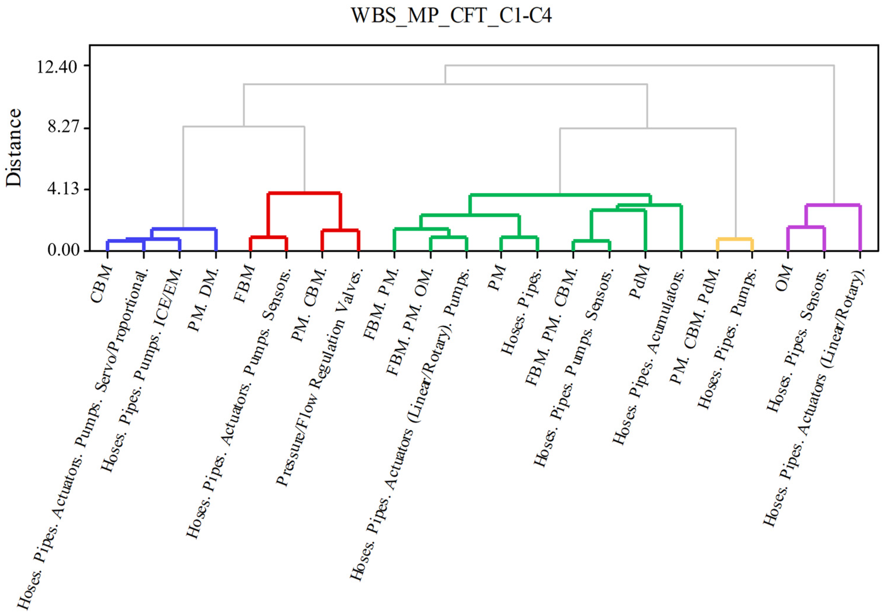
Total	1.000				1.435	1.000	1.000	1.000

) tables, it can be seen that only 8/20 components possess a quality of representation > 0.70. Therefore, at least 80.8% of inertia must be preserved; consequently, the fourth component is added.

The results (Figure 9) show that the first cluster (blue), consisting of {CBM} and {PM. DM.}, reports a variety of failures, alongside the second (red), where {FBM} and {PM. CBM.} report a smaller variety of failures. The third cluster (green) presents a higher association among the MPs. The fourth cluster (yellow) shows the smallest distance between the MPs {PM. CBM. PdM.} and the failures {Hoses. Pipes. Pumps.}, suggesting the best performance among the applications. Finally, the last cluster (purple) shows small distances between {OM} and ({Hoses. Pipes. Sensors.} and {Hoses. Pipes. Actuators}).

3.3. Relationship between MPs and RCFs Using CA-AHC

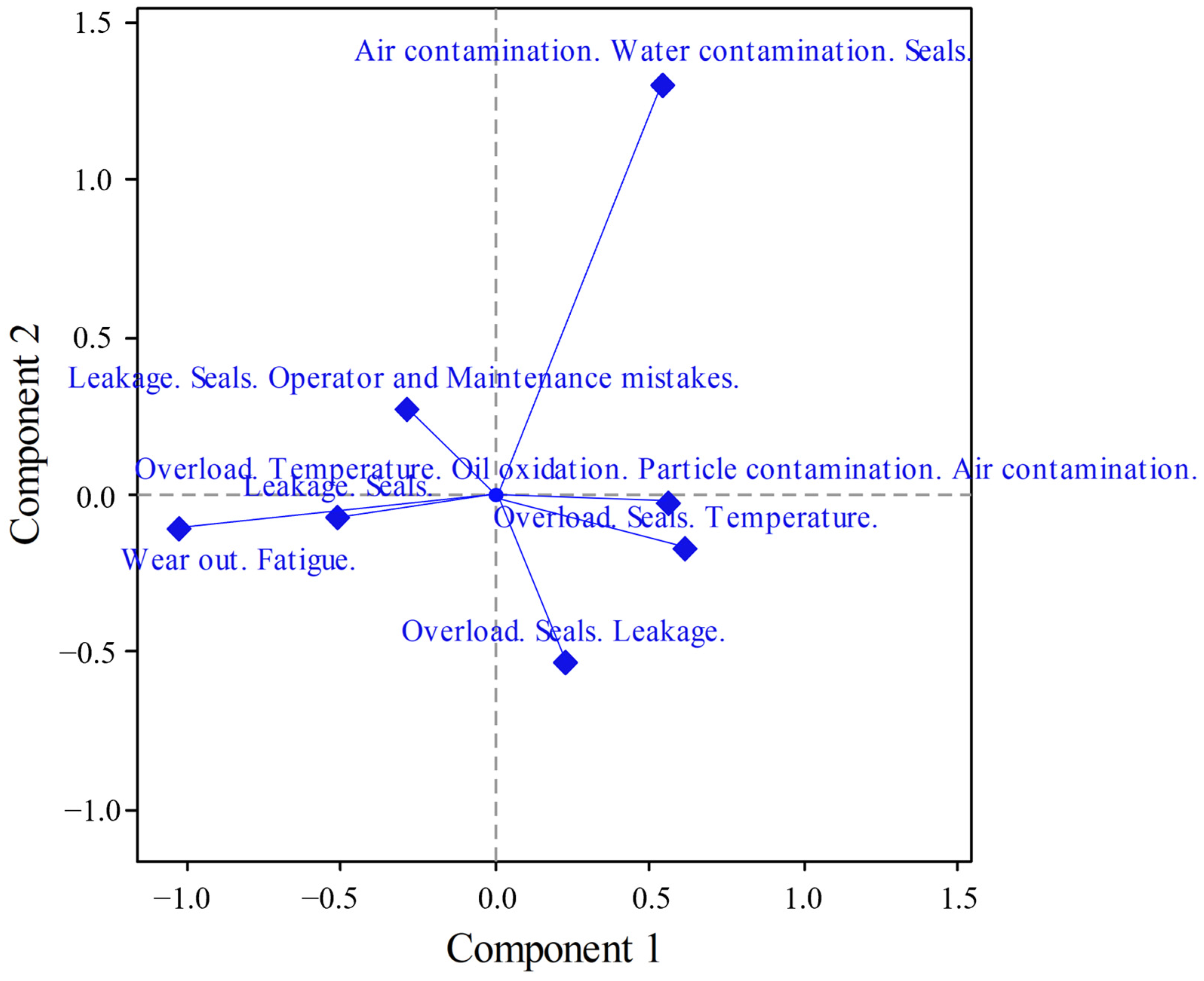
In terms of the RCF variable, the category of {Leakage. Seals. Operator and Maintenance mistakes.} was the most dominant. With regard to the frequency of the root causes reported, the highest-frequency f_ij association was that among {PdM} and OST {Overload. Seals. Temperature.} (f_PdM.OST = 0.667). Aside from failures associated with leakage and seals, operator/maintenance personnel mistakes were dominant in {PM. DM.} and {OM}.

The results show a statistically significant value (

Table 7. Quality of interpretation using MPs and RCFs.

Component	Inertia	Chi2	Sig.	Proportion of Inertia		Confidence Singular Value
				Accounted	Cumulative	C1	C2	C3
1	0.245			0.329	0.329	0.064	0.044	−0.450
2	0.196			0.262	0.591	0.090		0.144
3	0.124			0.166	0.757	0.081
4	0.113			0.151	0.909
5	0.052			0.070	0.979
6	0.016			0.021	1.000
Total	0.746	85.769	0.016	1.000	1.000

) of χ² = 85.769 (p = 0.016), which suggests the existance of a relationship between the categories. Compared to the previous case, the total inertia of Φ² = 0.746 with components C1-3 (75.7%) suggests better interpretability than MPs and CFTs (69.3%).

Observing the inertia of the row profiles (

Table 8. Row profile inertia of MPs and RCFs.

MP	Mass	C1	C2	C3	λ	Correlation			Contribution
						C1	C2	C3	C1	C2	C3	Qual
CBM	0.113	−0.436	0.245	0.135	0.065	0.088	0.035	0.016	0.329	0.104	0.031	0.465
FBM	0.096	−0.085	−0.166	0.309	0.024	0.003	0.013	0.074	0.029	0.111	0.386	0.525
FBM. PM.	0.104	0.072	0.570	0.707	0.095	0.002	0.173	0.420	0.006	0.357	0.549	0.911
FBM. PM. CBM.	0.096	−0.400	0.157	−0.60	0.063	0.062	0.012	0.275	0.242	0.037	0.541	0.820
FBM. PM. OM.	0.061	0.760	0.476	−0.10	0.067	0.143	0.071	0.005	0.526	0.206	0.010	0.742
OM	0.035	0.259	−1.78	0.532	0.127	0.010	0.566	0.079	0.018	0.870	0.077	0.966
PdM	0.026	0.985	0.658	−0.22	0.045	0.103	0.058	0.010	0.558	0.249	0.027	0.834
PM	0.330	0.347	−0.177	−0.18	0.075	0.163	0.053	0.083	0.532	0.139	0.137	0.809
PM. CBM.	0.052	−0.296	−0.008	−0.15	0.040	0.019	0.000	0.010	0.114	0.000	0.030	0.145
PM. CBM. PdM.	0.078	−1.11	−0.077	−0.08	0.116	0.395	0.002	0.005	0.835	0.004	0.005	0.844
PM. DM.	0.009	−0.588	−0.615	0.569	0.028	0.012	0.017	0.023	0.106	0.116	0.099	0.321
Total	1.000				0.746	1.000	1.000	1.000

), the selected components (dimensions) show that {OM} provides the highest percentage of variation λ_OM = 0.127 (17%), followed by {PM. CBM. PdM.} λ_PM.CBM.PdM = 0.116 (15.6%), and {FBM. PM.} λ_FBM.PM = 0.095 (12.7%). Looking at the Qual of the interpretation, it can be seen that for the suggested categories of row profiles, the selected components contributed greatly (Qual > 0.80) to the inertia.

Looking at the inertia by individual components (Figure 10), {OM} seems not to be associated with the previous points. Although {PM. CBM. PdM.} and {PdM} were closely associated in the previous analysis, the points here repel each other on C1. The biplot (Figure 10) provides significant insight without the explicit use of data.

The data (

Table 9. Column profile inertia of MPs and RCFs.

MP	Mass	C1	C2	C3	Inertia	Correlation for Column			Contribution
						C1	C2	C3	C1	C2	C3	Qual
AWCS	0.070	0.548	−1.306	0.175	0.149	0.085	0.607	0.017	0.140	0.796	0.014	0.950
LS	0.226	−0.509	0.073	−0.415	0.120	0.239	0.006	0.313	0.489	0.010	0.324	0.823
LSOMM	0.235	−0.291	−0.272	0.200	0.067	0.081	0.089	0.076	0.299	0.261	0.141	0.701
OSL	0.183	0.227	0.533	0.472	0.115	0.038	0.265	0.328	0.082	0.451	0.354	0.887
OST	0.209	0.618	0.170	−0.351	0.136	0.325	0.031	0.207	0.584	0.044	0.188	0.817
OTOPAW	0.035	0.562	0.021	0.126	0.045	0.045	0.000	0.004	0.243	0.000	0.012	0.256
WFF	0.043	−1.024	0.110	0.395	0.114	0.186	0.003	0.055	0.401	0.005	0.060	0.466
Total	1.000				0.746	1.000	1.000	1.000

) suggest that within the dimensions C1-3, {AWCS} has the highest inertia, λ_AWCS = 0.149, followed by {OST}, λ_AWCS = 0.136, and {LS}, λ_AWCS = 0.120. The Qual metric suggests that AWCS {Air contamination. Water contamination. Seals.} contains enough information for to be visualised (Qual_AWCS = 0.950).

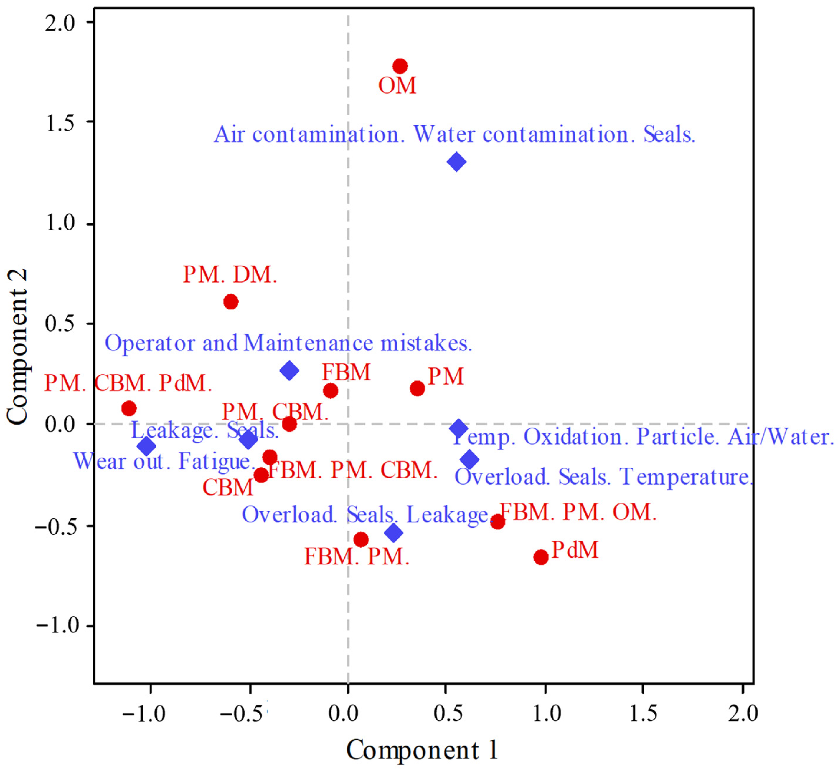
The graph (Figure 11) shows that C1 (the positive side) suggests that failures are associated with contamination, while the left side of C1 (the negative side) is associated with failures due to operator/maintenance mistakes. The results presented in the biplot (Figure 12) suggest a high association between {OM} and {Air/Water contamination. Seals.}. The positive sides of the C1-C2 components suggest an association among practices in which failures are reported due to contamination, while the centre and negative sides report a variety of failures.

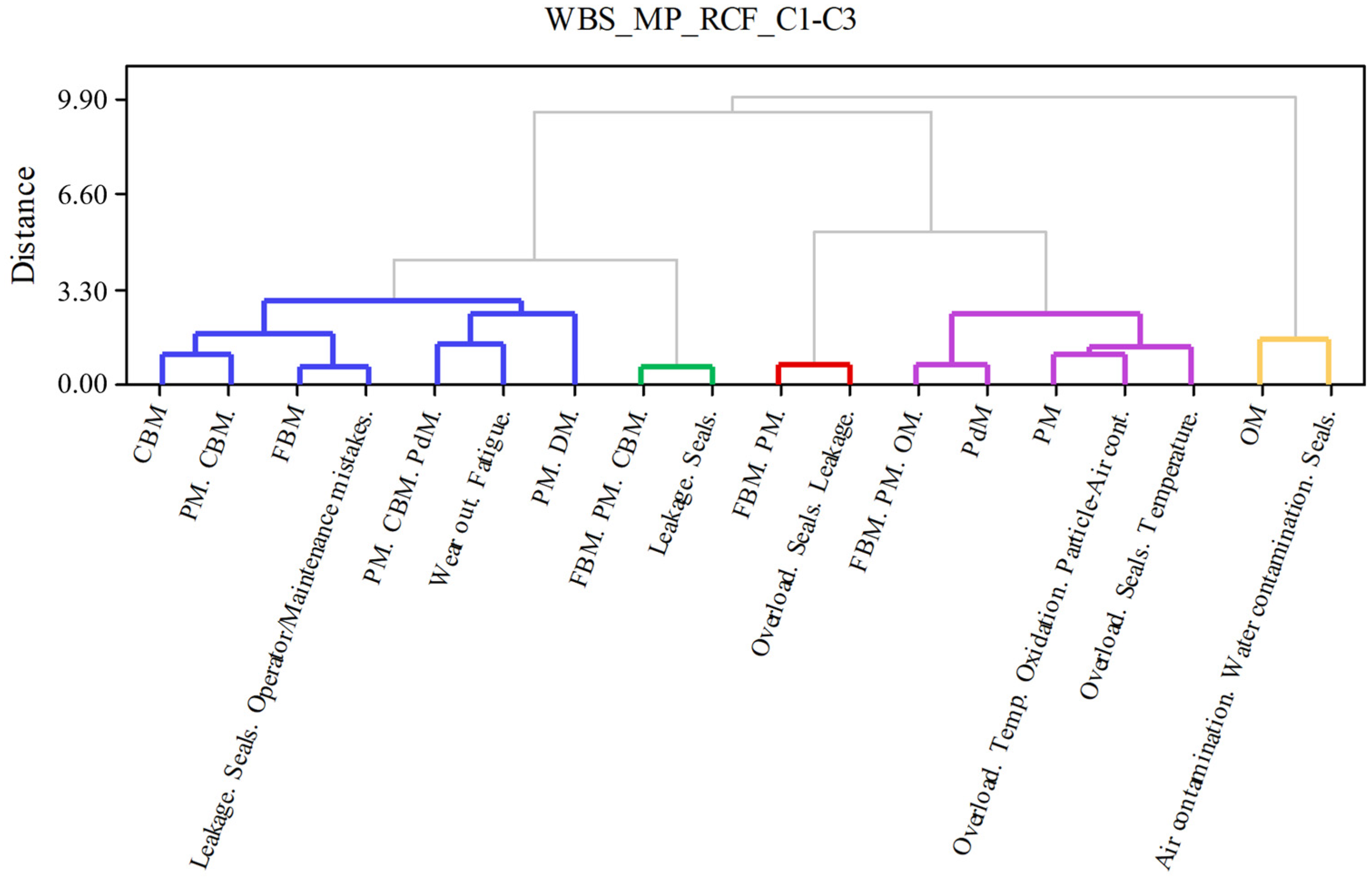
Considering an inertia of 75.7%, the representation shows that Qual > 0.70 contains 12/18 categories, while with the extension to the fourth component, all except {PM. DM.} have Qual > 0.70. Thus, interpretation using only three components (75.7% inertia) was sufficient. The first cluster (blue) on the dendrogram (Figure 13) had the most significant association between the MPs and failures associated with {Leakage. Seals. Operator and Maintenance Mistakes}, especially {FBM}. The second cluster (green) shows the smallest distance between {FBM. PM. CBM.} and {Leakage. Seals.}. The third (red) cluster shows similarity between {FBM. PM.} and {Overload. Seals. Leakage.}. The fourth (purple) cluster shows similarities among different applied MPs and failures related to overload and temperature. Finally, the last cluster (yellow) shows similarity between {OM} and {Air contamination. Water contamination. Seals.}.

3.4. Clusters and Performance Metrics

The obtained clusters (MP-CFT in

Table 10. MP-CFT clusters and performance metrics.

Metric	MTTR						MTBF						WOMM
Cluster	0 *	1	2	3	4	5	0 *	1	2	3	4	5	0 *	1	2	3	4	5
Med	5	3	5.1	5	5	4	950	550	1950	1500	1650	945.5	26.3	40.7	22.7	23.4	9.6	30.3
Mean	5.1	4.1	5.3	5.2	4.7	4	1196	907.1	1558	1495	1616	1010.2	39.8	39.8	41.2	27.9	30.1	30.3
Stdev	2.3	2.7	1.5	3.1	1.8	1.1	706.6	673.6	1157.7	735.5	728.8	655.5	45.6	19.1	50.2	26.1	26.7	1.1
Min	1	2	3	2	2	3	200	350	150	100	250	450	2.22	16.1	2.5	1.25	7.2	29.4
Max	12	10	7.5	15	8	5	2650	2500	2950	3500	2500	1700	250	71.43	136.3	142.9	62.5	31.2

* Clusters that were left out of the analysis.

and MP-RCF in

Table 11. MP-RCF clusters and performance metrics.

Metric	MTTR						MTBF						WOMM
Cluster	0 *	1	2	3	4	5	0 *	1	2	3	4	5	0 *	1	2	3	4	5
Med	5	5	3	5.5	4	3	1250	950	1995.5	950	1575	1570.5	26	36.5	19.4	11.9	31.3	29.4
Mean	5	5.1	3.5	6.9	4.7	3	1290.8	1087.5	2023.5	1341.7	1418.7	1570.5	36.1	41.3	19.2	29.5	27.6	29.4
Stdev	2.8	2	1.3	3.3	2.6	0	710.5	805.6	1096.3	651.5	745.4	183.1	40.3	28.9	5.9	39.3	19.5	0.00
Min	1	2	2	3.5	1	3	150	150	850	950	100	1441	2.20	2.50	12.2	7.10	1.30	29.4
Max	15	10	5.3	12	12	3	2950	2500	3500	2500	2750	1700	250	129.4	26.8	108.3	71.4	29.4

* Clusters that were left out of the analysis.

) were benchmarked against performance metrics, including both technical (i.e., MTTR, MTBF) and sustainability-related (e.g., WOMM) metrics. Although there was no significant variation among MTTR values with respect to clusters, the MTBF metric showed differences among the metrics. Namely, in both cases, clusters 2, 3, and 4 outperformed the other clusters, where the second cluster showed the best performance for the mean value of MTBF. Considering the WOMM metric, the results indicate that the second, third and fourth clusters possessed lower average WOMM. Note: The cluster 0* (n = 21) includes the respondents that were not clustered, and were left out of the analysis.

3.5. Machine Learning Feature Importance

To select machine learning algorithms, we checked the normality of data using the Shapiro–Wilk test. The test showed that the normality assumption was violated; thus, we used non-parametric ML algorithms including RF (Random Forest), SVM (Support Vector Machine), kNN (k-Neirest Neighbour) and DT (Decision Tree). The results of ML regression analysis for response MPIs of MTTR (

Table 12. Performance results of MTTR.

ML	RF	SVM	kNN	DT
MSE	3.412	1.009	4.846	877137.904
RMSE	1.847	1.004	2.201	936.556
MAE/MAD	1.314	0.627	1.694	767.94
R2	0.125	0.002	0.033	0.009

), MTBF (

Table 13. Performance results of MTBF.

ML	RF	SVM	kNN	DT
MSE	463982.999	833283.033	648621.198	877137.904
RMSE	681.163	912.843	805.37	936.556
MAE/MAD	584.637	712.324	633.333	767.94
R2	0.304	0.059	0.156	0.058

) and WOMM (

Table 14. Performance results of WOMM.

ML	RF	SVM	kNN	DT
MSE	853.157	991.228	1560.16	979.015
RMSE	29.209	31.484	39.499	31.289
MAE/MAD	22.789	23.051	27.713	20.396
R2	0.222	0.03	0.02	0.056

) are provided in the following. Additionally, the reason for selecting these non-parametric regression algorithms is that they can be used with continuous and categorical predictors. Finally, we used feature importance from the obtained results to allocate the most important predictors.

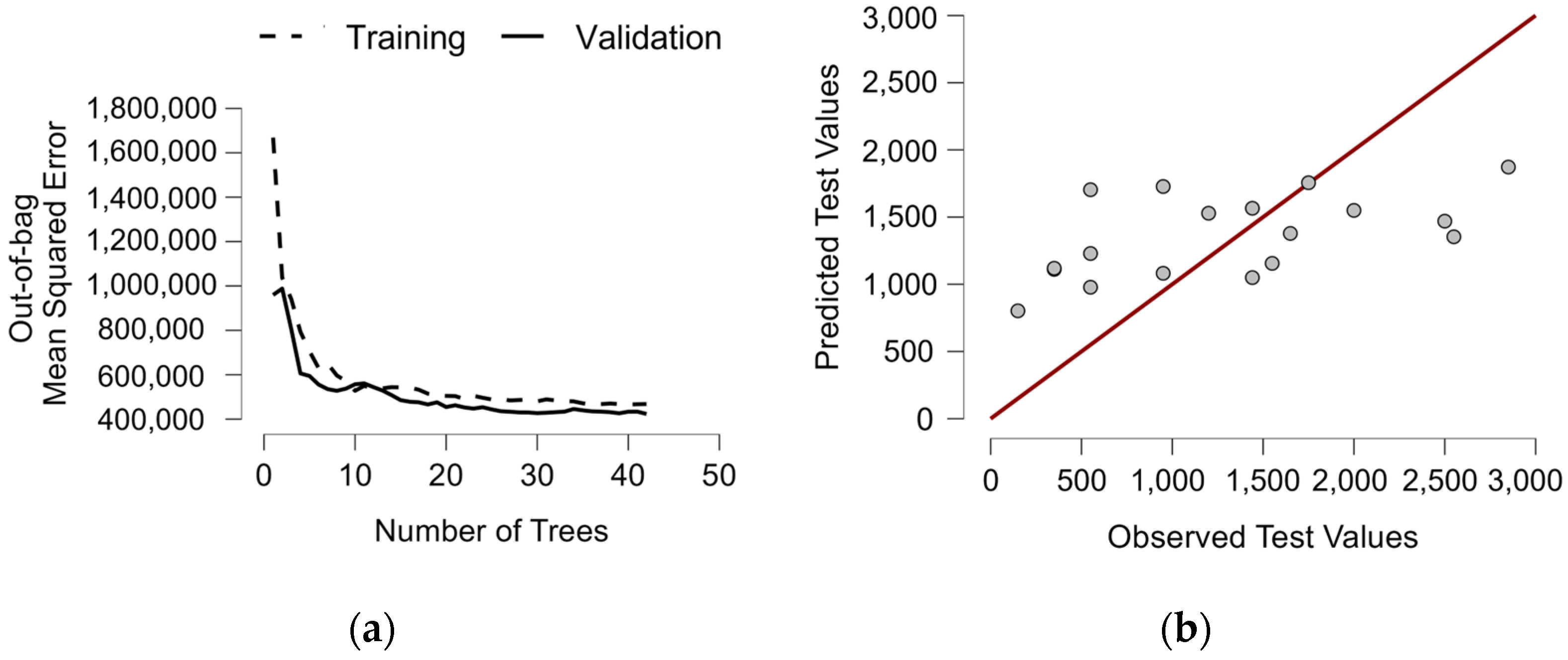
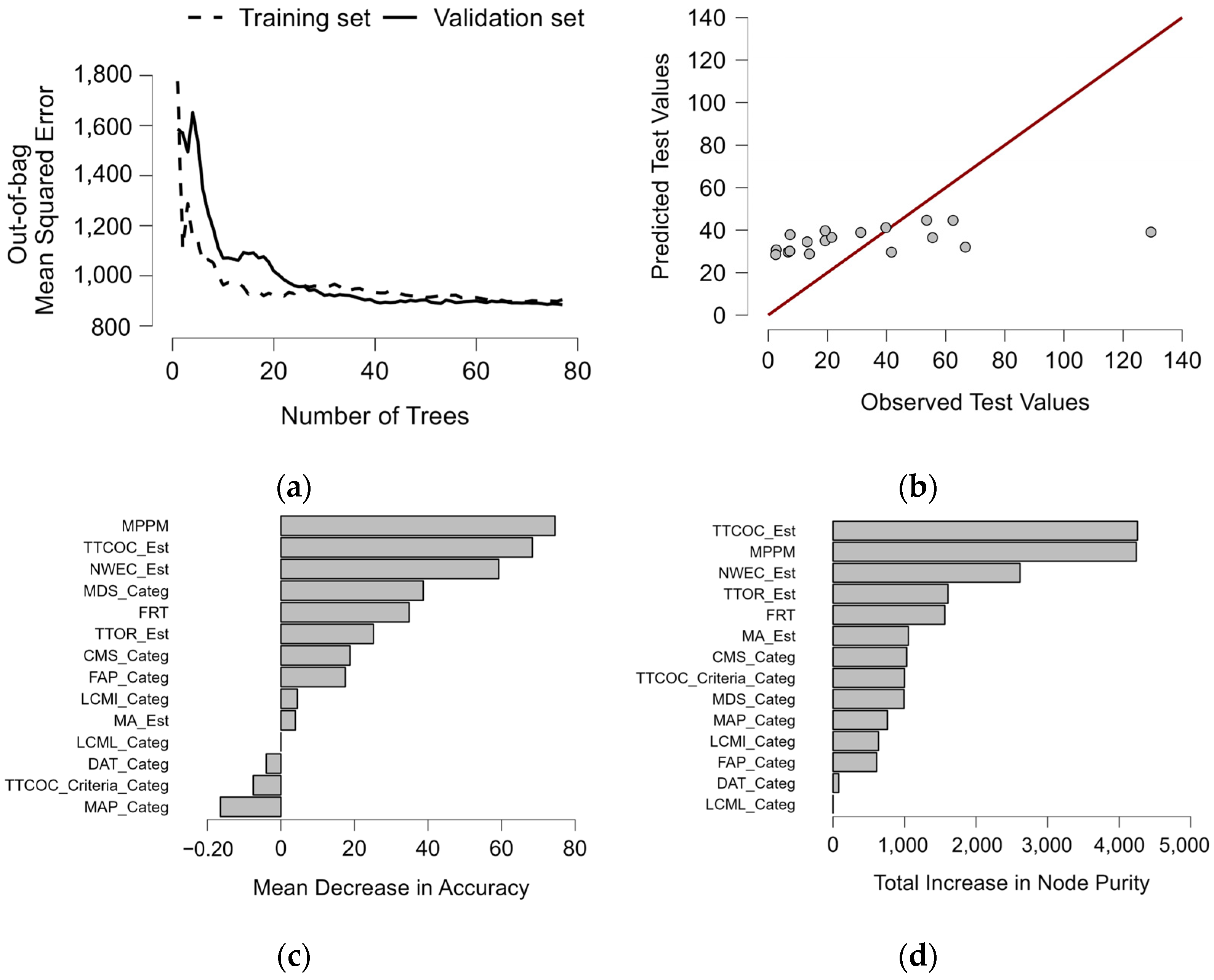
The results show that RF outperformed the other models. The out-of-bag MSE did not change significantly (Figure 14), and up to approximately 10 trees were enough to reduce the discrepancy between training and testing. However, a significant error existed in all cases due to the low prediction accuracy. The regression (Figure 14) showed significant variation in the validation (predicted vs. observed values). Feature perturbations were conducted to measure the mean decrease in accuracy, showing that MDS (Maintenance Department Staff), NWEC (Nominal Working Energy Consumption), TTCOC (Time To Complete Oil Change), MPPM, and FAP were the most essential features (Figure 14). Conversely, the increase in node purity (Figure 14) showed that NWEC, MPPM, and TTOR (Time To Oil Refilling) were the main contributors to the homogeneity of the output, i.e., the reduction in variance. In addition, negative features such as CMS (Condition Monitoring Sensor), TTCOC, and MA suggest noise and/or overfitting, calling into question their suitability for modelling, since they do not seem to contribute positively to prediction.

Considering the MTBF (Figure 15) metric, the evidence suggests that machine age has the highest impact on MTBF. This is also supported by empirical evidence [21], as equipment age contributes significantly to the reduction of MTBF. Additionally, MPPM, TTOR, TTCOC, MAP (Maintenance Analysis Program), and FRT (Filter Replacement Time) are the most critical indicators of MTBF. This suggests that hydraulic fluid condition significantly affects the MTBF of hydraulic machinery.

Observing the sustainability metric of WOMM, it can be seen that MPPM, TTCOC, NWEC, MDS, and FRT are the most impactful factors for fluid waste (Figure 16), with respect to both the reduction of MSE and the decrease in variance. To better understand this, we used the ranking of feature importance to establish essential features (Figure 17). The ranking showed that the number of maintenance personnel per machine played a vital role in hydraulic system maintenance, followed by time to oil refilling, the equipment size measured by nominal working energy consumption, machinery age, filter replacement time, etc. Surprisingly, although only 9.6% of the companies applied data analysis tools in hydraulic machine maintenance, only slight improvements were noticeable considering the output metrics. This is also for the case for the laboratory analysis of hydraulic oil, which showed no significant impact on the output metrics.

4. Discussion

4.1. Research Results from the Analysis of MPs and CFTs

The results show a high association between the investigated variables of MPs and CFTs, χ² = 165.021, with a p-value < 0.001. Looking at the categories of MPs, {PM} is the most frequently applied MP, while among CFTs, it is suggested that {Hoses. Pipes. Actuators. Pumps. Servo/Proportional valves.} is the most frequently reported category of component failures.

The results obtained show that the first cluster, {CBM} and {Pipes. Actuators. Pumps. DV (Servo/Proportional) valves.} with {Hoses. Pipes. Pumps. ICE/EM.}, suggests the poor performance of MPs. Namely, filtering {CBM} using different items, it turns out that companies that report using {CBM} strictly had the lowest MTBF_CBM = 835 h, and in that sense had the worst performance when considering this metric. The results show that maintenance activities behind {CBM} mostly included visual inspection (56%), while in up to 75% of the cases in which condition monitoring instruments like PFT (Pressure/Flow/Temperature) were used, they were not used for maintenance decision making. Considering data analysis, the results show that only 7% of {CBM} respondents report using data analysis tools. This also poses a question as to whether maintenance practitioners truly apply CBM and at what level. The second (red) and third (green) clusters show mixed MPs and a variety of reported failures, although with less severity and variation than in the first cluster. The fourth (yellow) and fifth (purple) clusters show presumably better performance in terms of reducing the severity of the failures of major components.

Taking a practical standpoint regarding the association between MPs and CFT using CA-AHC analysis, the results suggest that advanced maintenance practices, such as CBM and PdM, seem to result in a smaller variety of failures being reported, while at the same time there is an increased frequency of sensor failures. This can be attributed to the fact that sophisticated monitoring technology and instruments can avoid some serious failures. On the other hand, when applying traditional practices, such as FBM and PM, stoppages are primarily associated with failures associated with actuators and power units. This can suggest poor maintenance skills and the lack of the competence required to prevent this type of failure. The absence of such abilities leads to severe failures and a drop in productivity. Overall, the use of CA-AHC analysis in our case proved compelling due to its ability to transform categorical data into a feature subspace that can then be used for extracting relevant predictors against MPIs.

4.2. Results from the Analysis of MPs and RCFs

The results show the existence of a relationship between MPs and RCFs, χ² = 85.769 (p < 0.05). While {PM} was reported to be the most applied practice, {Leakage. Seals. Operator and Maintenance personnel mistakes.} was the most reported category of RCF, with leakage and seals being the most reported root causes of failure across categories.

The clusters obtained from the CA-AHC analysis suggest the following. The first (blue) cluster (Figure 13) shows similarity mostly between {CBM}, {PM. CBM.}, and {FBM}, and failures associated with {Leakage. Seals. Operator and Maintenance mistakes.} on one side, while at higher distances among categories of the same cluster, {PM. CBM. PdM.} and {PM. DM.} show an association with {Wear out. Fatigue.} of hydraulic components. Compared to other items from the survey considering quantitative data, the highest value of MTBF was indeed reported for {Wear out. Fatigue.}, where MTBF_{{Wear out. Fatigue}} = 2080 h.

Looking at the qualitative items, 60% of cases show the utilisation of Pressure/Flow/Temperature/Contamination sensors, suggesting that failures were avoided using an effective maintenance program. The second (green) cluster reports failures, mainly {Leakage. Seals.}, and displays similarity with {FBM. PM. CBM.}. Looking at the analysis of MPs and CFTs, these types of of practices show a small distance from {Hoses. Pipes. Pumps. Sensors}, suggesting CM practice; however, failures associated with leakage/seals could not be prevented. Unlike the previous cases, the third (red) and fourth (purple) clusters are similar to the failures associated with overload. This also justifies the failures associated with temperature, since overload leads to the transformation of power into heat and its subsequent dissipation. Finally, the last (yellow) cluster shows the similarity between {OM} and {Air/Water contamination. Seals.}, suggesting that these failures are associated with constant inspections and activities (e.g., filter replacements, oil refilling). Indeed, looking at quantitative data, MTTR_{{AirWater cont.}} = 6.13 h, which is the second-highest value (with operator/maintenance mistakes being the highest), which suggests that the long time required to perform a repair leaves the system exposed to the environment. The time required to complete an oil change was 3995 h on average, while usual practice and equipment manufacturers suggest approximately 2000 h. Additionally, the activity of TTOR, which is the application of usual maintenance activity to “refresh” the oil properties, is 191.7 h. This practice of trying to compensate for the loss of fluid properties (e.g., viscosity) and, consequently, system response by constantly adding fluid into the system is associated with oxidation and particle/air contamination.

Taken together, several conclusions can be derived. Firstly, the component failures and root causes of failure in hydraulic systems can be clustered into three categories: (1) Random events—these typically include failures of components such as pipes and hoses. This can also be said for failures associated with leakage and seals, since over 90% of companies report these failures. (2) Non-random events—these typically include degradational events under advanced maintenance practices. For instance, the failure of pumps and actuators for which pressure, flow and temperature indicators can explain or indicate degradational behaviour. Looking at RCF, non-random effects include failures associated with contamination in which instruments (e.g., particle counters) can be implemented to monitor and reduce the severity of wear. (3) Human-related events—the obtained evidence suggests a lack of industrial maintenance personnel, especially with respect to advanced data analytics and specialists in the domain of hydraulic system maintenance.

4.3. Feature Importance Considering Performance Metrics

The generated CA-AHC feature subspaces of the devised categories were used with the RF algorithm to extract relevant predictors, i.e., features related to MPIs. From an asset and machine perspective, equipment size (i.e., NWEC) and machine age seem to be the most important predictors. Introducing the NWEC variable for measuring the maintenance performance proved significant, and has not previously been reported in the literature, to the best of the authors’ knowledge. From a maintenance perspective, the number of maintenance personnel per machine, i.e., MPPM, has the greatest impact on the prediction properties of RF regression overall. This is also a vital remark since, to the best of the authors’ knowledge, no empirical evidence has been presented in the literature. Considering maintenance activities, TTOR, FRT, TTCOC, and TTCOC_Criteria, are the most essential features. Hence, considering the fact that fluid contamination is one of the most common causes of failure, the constant refilling of hydraulic oil and frequent complete oil changes in the system, presumably by overhaul, reduces the probability of failure, increasing MTBF and, at the same time, reducing the MTTR of the hydraulic machinery. From a technological perspective, LCMI (Lubricant Condition Monitoring Instruments) is the most critical feature overall; however, the impact on MTTR is questionable, unlike MTBF and WOMM, where it has a significant impact. Additionally, the CMS and LCML (Lubricant Condition Monitoring Laboratory) analyses show poor or negative predictive properties with respect to the performance metrics used in our analysis.

The allocated features that show a negative or poor contribution to the regression model suggest that the existing maintenance of hydraulic systems shows low technological and digital readiness levels. Namely, the fact that 45.2% of MDS consist only of operators and technicians calls into question whether companies perceive maintenance as a “strategic move”, or still see it as a “necessary evil”. Rhetorically, companies utilising advanced PdM solutions have faced difficulties in managing their assets, and as a result have reported a variety of failures. This, however, proved to be a business opportunity for companies and maintenance experts willing to engage with and provide outsourced maintenance services using in-house solutions, which is why many engage with MaaS (Maintenance as a Service) concepts [61]. Additionally, the results show that 13.1% of companies outsource their maintenance activities, while 50.4% rely on external experts or companies to perform equipment failure analysis. Moreover, confounding statistics regarding the application of data analysis show that only 9.6% of companies apply statistical or data analysis tools in hydraulic machine maintenance, which is why no actual contribution to the prediction properties was observed.

Important notice should be given to the ML algorithms used. Namely, considering that non-parametric regression ML algorithms were mainly chosen, with the violation of normality (Shapiro–Wilk p value > 0.05) and their ability to handle mixed data (categorical and continuous) being given as the rationale for their selection. However, other algorithms like gradient boosting machines (XGBoost and LightGBM) or even some neural networks can be used if the data are sufficient. Next, although we used RF feature importance to isolate important predictors, in complex models, tools like SHAP (SHapley Additive exPlanations) would also be of interest for explaining the performance outputs. Nevertheless, given the constraints of our dataset, we limited our exploration of other powerful parametric methods that might yield different insights when applied to different samples. This study relied heavily on data obtained from a questionnaire-based survey, which might inherently have some biases based on respondents applying day-to-day maintenance practices. Finally, deep learning methods that require extensive amounts of data for training were not considered due to the limited size of our dataset. With a more extensive dataset, the exploration of neural networks might provide additional insights through the benchmarking of existing maintenance practices.

5. Conclusions

This paper presented an extensive and in-depth study of features affecting the maintenance performance of companies utilising hydraulic machines. The study used empirical evidence and data synthesised from a questionnaire-based survey disseminated throughout the territory of the West-Balkan countries. Since extensive data were gathered, the study used correspondence analysis in combination with agglomerative hierarchical clustering to generate a feature subspace, after which components were used to identify the predictors impacting maintenance performance metrics, such as MTBF, MTTR and WOMM. The evidence shows that maintenance personnel, machine age, equipment size measured by nominal working energy consumption level, filter replacement time and time required to complete an oil change are the highest-ranked predictors, as established using the random forest algorithm.

Although the obtained evidence represents a significant contribution to the body of knowledge regarding hydraulic system maintenance, the study has limitations. Namely, the obtained results include a variety of companies under different NACE classifications; thus, the environmental conditions and working regimes can differ. Next, the results obtained via non-parametric ML algorithms due to violation of normality need to be further verified using a larger sample size. Additionally, further analysis needs to be conducted to verify and validate the impact of features on operational performance.

In the future, we plan to conduct a study regarding the impact of maintenance features on maintenance performance metrics, considering both categorical and numerical data. Specifically, we will include measuring the impact of outsourced versus in-house maintenance and the impact of data analysis tools in hydraulic machine maintenance. The underlying reason for this is the obvious barrier between preventive and predictive maintenance. The evidence also supports the need for more success in implementing advanced maintenance practices in this domain.