Article

Ambrosetti–Prodi Alternative for Coupled and Independent Systems of Second-Order Differential Equations

by
Feliz Minhós
1,2,* and
Gracino Rodrigues
2,3
1
Department of Mathematics, School of Science and Technology, University of Évora, Rua Romão Ramalho, 59, 7000-671 Évora, Portugal
2
Center for Research in Mathematics and Applications, Institute for Advanced Studies and Research, University of Évora, Rua Romão Ramalho, 59, 7000-671 Évora, Portugal
3
Coordination of Degree in Mathematics, Campus Maceió, Federal Institute of Education, Science and Technology of Alagoas, R. Mizael Domingues, 530, Centro, Maceió 57020-600, AL, Brazil
*
Author to whom correspondence should be addressed.
Mathematics 2023, 11(17), 3645; https://doi.org/10.3390/math11173645
Submission received: 30 July 2023 / Revised: 21 August 2023 / Accepted: 22 August 2023 / Published: 23 August 2023

Abstract

:
This paper deals with two types of systems of second-order differential equations with parameters: coupled systems with the boundary conditions of the Sturm–Liouville type and classical systems with Dirichlet boundary conditions. We discuss an Ambosetti–Prodi alternative for each system. For the first type of system, we present sufficient conditions for the existence and non-existence of its solutions, and for the second type of system, we present sufficient conditions for the existence and non-existence of a multiplicity of its solutions. Our arguments apply the lower and upper solutions method together with the properties of the Leary–Schauder topological degree theory. To the best of our knowledge, the present study is the first time that the Ambrosetti–Prodi alternative has been obtained for such systems with different parameters.

1. Introduction

This article focuses on the sufficient conditions that must be present from nonlinearities in order to be able to discuss, depending on the parameters, the existence and non-existence of solutions for second-order systems of the type
u 1 ( t ) + f ( t , u 1 ( t ) , u 2 ( t ) , u 1 ( t ) ) = μ v 1 ( t ) , u 2 ( t ) + g ( t , u 1 ( t ) , u 2 ( t ) , u 2 ( t ) ) = λ v 2 ( t ) ,
for t 0 , 1 , where f , g : 0 , 1 × R 3 R , v 1 , v 2 : 0 , 1 R + are continuous functions and μ , λ are real parameters, along with the boundary conditions
a i u i ( 0 ) b i u i ( 0 ) = 0 , c i u i ( 1 ) + d i u i ( 1 ) = 0 ,
where a i , b i , c i , d i 0 ,   i = 1 , 2 , such that a i + b i > 0 and c i + d i > 0 .
A multiplicity of solutions will be obtained for a particular case of (1) and (2), that is,
u 1 ( t ) + f ( t , u 1 ( t ) , u 1 ( t ) ) = μ v 1 ( t ) , u 2 ( t ) + g ( t , u 2 ( t ) , u 2 ( t ) ) = λ v 2 ( t ) ,
for t 0 , 1 , where f , g : 0 , 1 × R 2 R , with the boundary conditions
u i ( 0 ) = u i ( 1 ) = 0 , for i = 1 , 2 .
These types of equations were introduced in [1], and since then, they have been studied by many authors in the context of different types of boundary value problems. As examples, we refer to [2,3] for three-point and two-point boundary value problems; ref. [4,5] for Neumann boundary conditions; ref. [6,7,8,9,10] for periodic problems; ref. [11] for parametric problems with ( p , q ) -Laplacian equations; ref. [12] for asymptotic conditions; and [13] for coercivity conditions.
Common to all of these problems is the discussion of the so-called Ambrosetti–Prodi alternative, in which there are some values, ξ 0 and ξ 1 , of a parameter ξ such that the problem has no solution for ξ < ξ 0 , at least one solution if ξ = ξ 0 , or two solutions if ξ 0 < ξ < ξ 1 .
Coupled systems of second-order differential equations, where there is dependence between the various unknown variables, were studied in a huge variety of theoretical and applied situations involving different types of boundary conditions, such as [14,15,16,17]. Moreover, there are many real phenomena modeled by coupled systems, particularly in problems related to population dynamics, as in [18,19,20,21].
Recently, in [22], the authors presented a technique to discuss the existence of coupled systems of two Ambrosetti–Prodi-type second-order fully differential equations and proved the existence of solutions for the values of the parameters for which there are lower and upper solutions for the system.
This paper extends, for the first time, as far as we know, the Ambrosetti–Prodi alternative to coupled systems of differential equations with two parameters. The existence and nonexistence of solutions are obtained for Problems (1) and (2), and a discussion of multiplicity for particular cases of the boundary conditions are considered in [22].
Our method relies on the lower and upper solutions technique together with a Nagumo condition to estimate the values of the first derivatives. Leray–Schauder topological degree properties play a key role in obtaining the multiplicity of solutions. As is usual in this type of method, the results also provide the localization for such solutions in a strip bounded by lower and upper solutions. This feature is particularly useful in practice, particularly in the application of these theorems to the study of population dynamics and namely to Lotka–Volterra steady-state systems with migration, as we show in the last section.
The paper is organized as follows. Section 2 contains definitions and some auxiliary results, such as the a priori Nagumo estimation for the first derivatives and a previous result used in the main results. The third and fourth sections provide a discussion of the two parameters for the existence and multiplicity of solutions, respectively. The last section presents an application for studying the interactions between two species under two scenarios: mutualism and neutralism.

2. Definitions and Auxiliary Results

In this section, some definitions, lemmas, and theorems are introduced for the subsequent analysis.
Let X = C 1 [ 0 , 1 ] be the usual Banach space equipped with the norm · C 1 , defined by
x C 1 : = max { x , x } ,
where
x : = max t [ 0 , 1 ] | x ( t ) | ,
and let X 2 = C 1 [ 0 , 1 ] × C 1 [ 0 , 1 ] with the norm
( x , y ) X 2 = max { x C 1 , y C 1 } .
The Nagumo condition, introduced by [23], establishes an a priori estimation for the first derivative of the solution of System (1), provided that it satisfies an adequate framework.
Definition 1. 
Let α i ( t ) , β i ( t ) , i = 1 , 2 be continuous functions such that
α i ( t ) β i ( t ) , for all t [ 0 , 1 ] ,
and consider the set
S = { ( t , y 1 , y 2 , y 3 ) [ 0 , 1 ] × R 3 : α 1 ( t ) y 1 β 1 ( t ) , α 2 ( t ) y 2 β 2 ( t ) } .
A continuous function h : [ 0 , 1 ] × R 3 R satisfies a Nagumo-type condition in the set (6) if there is a continuous positive function φ : [ 0 , + ) ( 0 , + ) satisfying
| h ( t , y 1 , y 2 , y 3 ) | φ ( | y 3 | ) ,
such that
0 + d s φ ( s ) = + .
The a priori estimate for the first derivatives is given by the next lemma following the arguments of [22].
Lemma 1. 
Suppose that the continuous functions f , g : [ 0 , 1 ] × R 3 R satisfy the Nagumo-type Conditions (7) and (8) in S. Then, for every solution ( u 1 , u 2 ) ( C 2 [ 0 , 1 ] ) 2 of (1) satisfying
α 1 ( t ) u 1 ( t ) β 1 ( t ) , and α 2 ( t ) u 2 ( t ) β 2 ( t ) , t [ 0 , 1 ] ,
there are N 1 > 0 and N 2 > 0 such that
u 1 N 1 , and u 2 N 2 .
Remark 1. 
The constant N 1 depends only on the parameter μ and on the functions v 1 , α 1 , and β 1 . Analogously, N 2 depends only on λ , v 2 , α 2 , and β 2 . However, if the parameters μ and λ belong to bounded sets, N 1 and N 2 can be taken independently of μ and λ.
To apply the lower and upper solutions method, depending on the values of the parameters μ and λ , we take the followings coupled functions.
Definition 2. 
Let a i , b i , c i , d i 0 such that a i + b i > 0 and c i + d i > 0 for i = 1 , 2 .
A pair of functions ( γ 1 , γ 2 ) ( C 2 ( ] 0 , 1 [ ) C 1 ( [ 0 , 1 ] ) ) 2 is a lower solution of Problems (1) and (2) if, for all t 0 , 1 ,
γ 1 ( t ) + f ( t , γ 1 ( t ) , γ 2 ( t ) , γ 1 ( t ) ) μ v 1 ( t ) , γ 2 ( t ) + g ( t , γ 1 ( t ) , γ 2 ( t ) , γ 2 ( t ) ) λ v 2 ( t ) ,
and, for i = 1 , 2 ,
a i γ i ( 0 ) b i γ i ( 0 ) 0 , c i γ i ( 1 ) + d i γ i ( 1 ) 0 .
A pair of functions ( ϕ 1 , ϕ 2 ) ( C 2 ( ] 0 , 1 [ ) C 1 ( [ 0 , 1 ] ) ) 2 is an upper solution of Problems (1) and (2) if, for all t 0 , 1 ,
ϕ 1 ( t ) + f ( t , ϕ 1 ( t ) , ϕ 2 ( t ) , ϕ 1 ( t ) ) μ v 1 ( t ) , ϕ 2 ( t ) + g ( t , ϕ 1 ( t ) , ϕ 2 ( t ) , ϕ 2 ( t ) ) λ v 2 ( t ) ,
and, for i = 1 , 2 ,
a i ϕ i ( 0 ) b i ϕ i ( 0 ) 0 , c i ϕ i ( 1 ) + d i ϕ i ( 1 ) 0 .
The first theorem is an existence and localization result that is a particular case of Theorem 3.1 of [22]. In short, it guarantees the existence of a solution for the values of μ and λ such that there are lower and upper solutions of Problems (1) and (2).
Theorem 1. 
Let f , g : [ 0 , 1 ] × R 3 R be continuous functions. If there are lower and upper solutions of (1) and (2), ( γ 1 , γ 2 ) and ( ϕ 1 , ϕ 2 ) , respectively, according to Definition 2, such that
γ i ( x ) ϕ i ( x ) , i = 1 , 2 , x [ 0 , 1 ] ,
and f and g satisfy Nagumo conditions as in Definition 1 relative to the intervals [ γ 1 ( x ) , ϕ 1 ( x ) ] and [ γ 2 ( x ) , ϕ 2 ( x ) ] for all x 0 , 1 with
f ( x , y 0 , z 0 , y 1 ) nondecreasing in z 0 ,
for x 0 , 1 , we have
min min x 0 , 1 γ 1 ( x ) , min x 0 , 1 ϕ 1 ( x ) y 1 max max x 0 , 1 γ 1 ( x ) , max x 0 , 1 ϕ 1 ( x ) ,
and with
g ( x , y 0 , z 0 , z 1 ) nondecreasing in y 0
for x 0 , 1 , we have
min min x 0 , 1 γ 2 ( x ) , min x 0 , 1 ϕ 2 ( x ) z 1 max max x 0 , 1 γ 2 ( x ) , max x 0 , 1 ϕ 2 ( x ) .
Then there is at least ( u ( x ) , v ( x ) ) ( C 2 [ 0 , 1 ] ) 2 , a paired solution of (1) and (2), and, moreover,
γ 1 ( x ) u ( x ) ϕ 1 ( x ) , γ 2 ( x ) v ( x ) ϕ 2 ( x ) , x [ 0 , 1 ] .

3. Existence and Non-Existence of Solutions

A preliminary discussion of the values of the parameters μ and λ , for which it is possible to guarantee the existence and non-existence of a solution for System (1) with the boundary Condition (2), is given by the next theorem.
Theorem 2. 
Let f , g : [ 0 , 1 ] × R 3 R be continuous functions fulfilling the conditions of Theorem 1. If we have μ 1 , λ 1 R , p > 0 , and q > 0 such that satisfy
f ( t , 0 , 0 , 0 ) v 1 ( t ) < μ 1 < f ( t , y 1 , y 2 , 0 ) v 1 ( t ) ,
for every t 0 , 1 ,   y 1 p , and y 2 R and
g ( t , 0 , 0 , 0 ) v 2 ( t ) < λ 1 < g ( t , y 1 , y 2 , 0 ) v 2 ( t ) ,
for every t 0 , 1 ,   y 1 R , and y 2 q , then there exist μ 0 < μ 1 and λ 0 < λ 1 (with the possibility of μ 0 = and λ 0 = ) such that:
1.
If μ < μ 0 or λ < λ 0 , there is no solution to (1) or (2);
2.
If μ 0 < μ μ 1 and λ 0 < λ λ 1 , then there is at least one solution to (1) and (2).
Proof. 
Claim 1: There exist  μ ¯ < μ 1 and  λ * < λ 1 such that (1) and (2) have a solution for  μ = μ ¯ and  λ = λ * .
Defining
μ ¯ : = max t [ 0 , 1 ] f ( t , 0 , 0 , 0 ) v 1 ( t ) , and λ * : = max t [ 0 , 1 ] g ( t , 0 , 0 , 0 ) v 2 ( t ) ,
there are t ¯ , t * [ 0 , 1 ] such that
f ( t , 0 , 0 , 0 ) v 1 ( t ) μ ¯ = f ( t ¯ , 0 , 0 , 0 ) v 1 ( t ¯ ) < μ 1 ,
and
g ( t , 0 , 0 , 0 ) v 2 ( t ) λ * = g ( t * , 0 , 0 , 0 ) v 2 ( t * ) < λ 1 ,
for all t [ 0 , 1 ] .
Then, the functions ϕ 1 ( t ) 0 and ϕ 2 ( t ) 0 are upper solutions of Problems (1) and (2) for μ = μ ¯ and λ = λ * . On the other hand, γ 1 ( t ) = p and γ 2 ( t ) = q are lower solutions of Problems (1) and (2) for μ = μ ¯ and λ = λ * since, by (18) and the boundary conditions, we have
  • γ 1 ( t ) = 0 > μ 1 v 1 ( t ) f ( t , p , q , 0 ) > μ ¯ v 1 ( t ) f ( t , p , q , 0 ) ,
  • γ 2 ( t ) = 0 > λ 1 v 2 ( t ) g ( t , p , q , 0 ) > λ * v 2 ( t ) g ( t , p , q , 0 ) ,
  • a 1 p 0 , and c 1 p 0 ,
  • a 2 q 0 , and c 2 q 0 .
As f and g satisfy the Nagumo conditions on the set
S 1 = { ( t , y 1 , y 2 , y 3 ) [ 0 , 1 ] × R 3 : p y 1 0 , q y 2 0 } ,
then, by Theorem 1, there exists at least one solution of Problems (1) and (2) for μ = μ ¯ < μ 1 and λ = λ * < λ 1 .
  • Claim 2: If (1) and (2) have a solution for μ = σ < μ 1 and  λ = ρ < λ 1 , then they have a solution for  μ [ σ , μ 1 ] , and  λ [ ρ , λ 1 ] .
Let ( u 1 σ ( t ) , u 2 ρ ( t ) ) be a solution of Problems (1) and (2) for μ = σ < μ 1 and let λ = ρ < λ 1 ; that is,
u 1 σ ( t ) + f ( t , u 1 σ ( t ) , u 2 ρ ( t ) , u 1 σ ( t ) ) = σ v 1 ( t ) , u 2 ρ ( t ) + g ( t , u 1 σ ( t ) , u 2 ρ ( t ) , u 2 ρ ( t ) ) = ρ v 2 ( t ) .
The pair of functions ( u 1 σ ( t ) , u 2 ρ ( t ) ) is an upper solution of (1) and (2) for values of μ and λ such that σ μ μ 1 and ρ λ λ 1 since
u 1 σ ( t ) = σ v 1 ( t ) f ( t , u 1 σ ( t ) , u 2 ρ ( t ) , u 1 σ ( t ) ) μ v 1 ( t ) f ( t , u 1 σ ( t ) , u 2 ρ ( t ) , u 1 σ ( t ) ) ,
and
u 2 ρ ( t ) = ρ v 2 ( t ) g ( t , u 1 σ ( t ) , u 2 ρ ( t ) , u 2 ρ ( t ) ) λ v 2 ( t ) g ( t , u 1 σ ( t ) , u 2 ρ ( t ) , u 2 ρ ( t ) ) ,
when the boundary conditions are trivially checked.
For p > 0 and q > 0 , as defined in (23) and (24), consider values of P > 0 and Q > 0 large enough such that
P p , Q q , u 1 σ ( 0 ) P , u 1 σ ( 1 ) P , u 2 ρ ( 0 ) Q , and u 2 ρ ( 1 ) Q .
Then, ( P , Q ) is a lower solution of Problems (1) and (2) for μ μ 1 and λ λ 1 since, by (18) and the boundary conditions, we have
  • 0 > μ 1 v 1 ( t ) f ( t , P , Q , 0 ) μ v 1 ( t ) f ( t , P , Q , 0 ) ,
  • 0 > λ 1 v 2 ( t ) g ( t , P , Q , 0 ) λ v 2 ( t ) g ( t , P , Q , 0 ) ,
  • a 1 P 0 , and c 1 P 0 ,
  • a 2 Q 0 , and c 2 Q 0 .
To apply Theorem 1, it remains to justify that
P u 1 σ ( t ) , and Q u 2 ρ ( t ) , t [ 0 , 1 ] .
Assume, by contradiction, that the first inequality is not satisfied. Then, there exists t [ 0 , 1 ] such that u 1 σ ( t ) < P , and we can define
min t [ 0 , 1 ] u 1 σ ( t ) : = u 1 σ ( t 0 ) < P .
By (20), u 1 σ ( t 0 ) = 0 , u 1 σ ( t 0 ) 0 , and, by (18), we obtain the contradiction
0 u 1 σ ( t 0 ) = σ v 1 ( t 0 ) f ( t 0 , u 1 σ ( t 0 ) , u 2 ρ ( t 0 ) , 0 ) μ v 1 ( t 0 ) f ( t 0 , u 1 σ ( t 0 ) , u 2 ρ ( t 0 ) , 0 ) μ 1 v 1 ( t 0 ) f ( t 0 , u 1 σ ( t 0 ) , u 2 ρ ( t 0 ) , 0 ) < 0 .
Then, P u 1 σ ( t ) for all t [ 0 , 1 ] .
Using a similar method, by (19), it can be shown that Q u 2 ρ ( t ) for all t [ 0 , 1 ] .
Therefore, by Theorem 1, there exists at least one solution ( u 1 ( t ) , u 2 ( t ) ) of Problems (1) and (2) for values of μ and λ such that μ [ σ , μ 1 ] and λ [ ρ , λ 1 ] .
  • Claim 3: There exist  μ 0 and  λ 0 such that:
For  μ < μ 0   or  λ < λ 0 , (1) and (2) have no solution;
for  μ 0 < μ μ 1   and  λ 0 < λ λ 1 , (1) and (2) have at least one solution.
Consider the set
A = { ( μ , λ ) R 2 : ( 1 ) and ( 2 ) has solution } ,
with the order relationship given by
x , y z , w x z y w .
The set A is not empty because, by Claim 1, ( μ ¯ , λ * ) A , and we can thus define
( μ 0 , λ 0 ) : = inf A .
If (1) and (2) have a solution for all μ < μ 1 and λ < λ 1 , then μ 0 = and λ 0 = .
By Claim 1 and (22), μ 0 μ ¯ < μ 1 and λ 0 λ * < λ 1 . By Claim 2, (1) and (2) have at least one solution for values of μ and λ such that μ 0 < μ μ 1 and λ 0 < λ λ 1 . □
Replacing f, g, y 1 , and y 2 with f , g , y 1 , and y 2 , respectively, in Conditions (18) and (19), we obtain a dual version of the previous theorem, whose proof follows the same type of arguments.
Theorem 3. 
Let f , g : [ 0 , 1 ] × R 3 R be continuous functions fulfilling the assumptions of Theorem 1.
If there are μ 1 , λ 1 R , p > 0 , and q > 0 that satisfy
f ( t , 0 , 0 , 0 ) v 1 ( t ) > μ 1 > f ( t , y 1 , y 2 , 0 ) v 1 ( t ) ,
for every t 0 , 1 ,   y 1 p and y 2 R ,
g ( t , 0 , 0 , 0 ) v 2 ( t ) > λ 1 > g ( t , y 1 , y 2 , 0 ) v 2 ( t ) ,
for every t 0 , 1 ,   y 1 R , and y 2 q , then there exists μ 0 > μ 1 and λ 0 > λ 1 (with the possibility of μ 0 = + and λ 0 = + ) such that the following hold true:
1.
If μ > μ 0 or λ > λ 0 , (1) and (2) have no solution;
2.
If μ 0 > μ μ 1 and λ 0 > λ λ 1 , (1) and (2) have at least one solution.

4. Multiplicity of Solutions

The multiplicity result is obtained for a particular case of Problems (1) and (2), namely, a standard system where the differential equations are independent with f , g : 0 , 1 × R 2 R .
The arguments are based on the topological Leray–Schauder degree, along with strict lower and upper solutions, as in the next definition.
Definition 3. 
i.
A pair of functions ( γ 1 , γ 2 ) ( C 2 ( ] 0 , 1 [ ) C 1 ( [ 0 , 1 ] ) ) 2 is a strict lower solution of Problems (3) and (4) if, for all t 0 , 1 ,
γ 1 ( t ) + f ( t , γ 1 ( t ) , γ 1 ( t ) ) > μ v 1 ( t ) , γ 2 ( t ) + g ( t , γ 2 ( t ) , γ 2 ( t ) ) > λ v 2 ( t ) ,
and
γ i ( 0 ) < 0 , γ i ( 1 ) < 0 , for i = 1 , 2 .
ii.
A pair of functions ( ϕ 1 , ϕ 2 ) ( C 2 ( ] 0 , 1 [ ) C 1 ( [ 0 , 1 ] ) ) 2 is a strict upper solution of Problems (3) and (4) if, for all t 0 , 1 ,
ϕ 1 ( t ) + f ( t , ϕ 1 ( t ) , ϕ 1 ( t ) ) < μ v 1 ( t ) , ϕ 2 ( t ) + g ( t , ϕ 2 ( t ) , ϕ 2 ( t ) ) < λ v 2 ( t ) ,
and
ϕ i ( 0 ) > 0 , ϕ i ( 1 ) > 0 , for i = 1 , 2 .
For the functional framework, we define the operators
L : ( C 2 ( [ 0 , 1 ] ) ) 2 ( C ( [ 0 , 1 ] ) ) 2 × R 4
given by
L ( u 1 , u 2 ) = ( u 1 , u 2 , u 1 ( 0 ) , u 1 ( 1 ) , u 2 ( 0 ) , u 2 ( 1 ) )
and
N ( μ , λ ) : ( C 1 ( [ 0 , 1 ] ) ) 2 ( C ( [ 0 , 1 ] ) ) 2 × R 4
given by
N ( μ , λ ) ( u 1 , u 2 ) = ( X , Y , 0 , 0 , 0 , 0 )
as
X : = θ f ( t , δ 1 ( t , u 1 ( t ) ) , u 1 ( t ) ) + u 1 ( t ) + θ [ μ v 1 ( t ) δ 1 ( t , u 1 ( t ) ) ] ,
and
Y : = ϑ g ( t , δ 2 ( t , u 2 ( t ) ) , u 2 ( t ) ) + u 2 ( t ) + ϑ [ λ v 2 ( t ) δ 2 ( t , u 2 ( t ) ) ] .
Since L is invertible, we can define the completely continuous operator
T : ( C 2 ( [ 0 , 1 ] ) ) 2 ( C ( [ 0 , 1 ] ) ) 2
given by
T ( θ , ϑ ) ( u 1 , u 2 ) = L 1 N ( μ , λ ) ( u 1 , u 2 ) .
Clearly, the operator T is compact, and the following lemma allows us to evaluate the topological degree, d ( I T , Ω , 0 , 0 ) .
Lemma 2. 
Assume that there are strict lower and upper solutions of (3) and (4), γ i ( t ) , and ϕ i ( t ) , respectively, with
γ i ( t ) < ϕ i ( t ) , i = 1 , 2 , t [ 0 , 1 ] ,
where the continuous functions f , g : [ 0 , 1 ] × R 2 R satisfy the Nagumo conditions as in Definition 1 relative to the intervals [ γ 1 ( t ) , ϕ 1 ( t ) ] and [ γ 2 ( t ) , ϕ 2 ( t ) ] .
Then, there is M > 0 such that, for
Ω = ( u 1 , u 2 ) ( C 2 ( [ 0 , 1 ] ) ) 2 : γ i ( t ) < u i ( t ) < ϕ i ( t ) , u i < M , i = 1 , 2 ,
we have
d ( I T ( 1 , 1 ) , Ω , 0 , 0 ) = ± 1 .
Remark 2. 
By Remark 1, it is possible to consider the same set Ω for Equation (3) regardless of μ and λ, provided that γ i ( t ) and ϕ i ( t ) are strict lower and upper solutions of (3) and (4) and ( μ , λ ) belongs to a bounded set.
Proof. 
Consider the truncated functions δ i : [ 0 , 1 ] × R R , i = 1 , 2 ,
δ i ( t , y i ) : = ϕ i ( t ) if y i > ϕ i ( t ) , y i if γ i ( t ) y i ϕ i ( t ) , γ i ( t ) if y i < γ i ( t ) .
For θ , ϑ [ 0 , 1 ] , consider the homotopic, truncated, and perturbed problem composed by the system
u 1 ( t ) + θ f ( t , δ 1 ( t , u 1 ( t ) ) , u 1 ( t ) ) = u 1 ( t ) + θ [ μ v 1 ( t ) δ 1 ( t , u 1 ( t ) ) ] , u 2 ( t ) + ϑ g ( t , δ 2 ( t , u 2 ( t ) ) , u 2 ( t ) ) = u 2 ( t ) + ϑ [ λ v 2 ( t ) δ 2 ( t , u 2 ( t ) ) ] ,
and the boundary Condition (4).
With these definitions, Problems (31) and (4) are equivalent to the operator equation
T ( θ , ϑ ) ( u 1 , u 2 ) = ( u 1 , u 2 ) .
For i = 1 , 2 , take R i > 0 such that, for every t [ 0 , 1 ] ,
R i < γ i ( t ) ϕ i ( t ) < R i , μ v 1 ( t ) f ( t , γ 1 ( t ) , 0 ) R 1 γ 1 ( t ) < 0 , μ v 1 ( t ) f ( t , ϕ 1 ( t ) , 0 ) + R 1 ϕ 1 ( t ) > 0 , λ v 2 ( t ) g ( t , γ 2 ( t ) , 0 ) R 2 γ 2 ( t ) < 0 , λ v 2 ( t ) g ( t , ϕ 2 ( t ) , 0 ) + R 2 ϕ 2 ( t ) > 0 .
By Lemma 1, and applying the technique suggested in the proof of Theorem 1 (see [22], Theorem 3.1) adapted to strict lower and upper solutions γ i ( t ) , and ϕ i ( t ) , there are positive real numbers M i , where i = 1 , 2 such that
u 1 < M 1 , and u 2 < M 2 ,
independently of the parameters θ and ϑ .
If we define
Ω 1 = { ( u 1 , u 2 ) ( C 2 ( [ 0 , 1 ] ) ) 2 : u i < R i , u i < M i , i = 1 , 2 } ,
then every solution of (32) belongs to Ω 1 for all θ , ϑ 0 , 1 2 ,   ( u 1 , u 2 ) Ω 1 , and, so, the degree d ( I T ( θ , ϑ ) , Ω 1 , 0 , 0 ) is well-defined for every θ , ϑ 0 , 1 2 .
For θ , ϑ = ( 0 , 0 ) , the equation T ( 0 , 0 ) ( u 1 , u 2 ) = ( u 1 , u 2 ) , that is, the homogeneous linear problems
u i ( t ) u i ( t ) = 0 , u i ( 0 ) = 0 , u i ( 1 ) = 0 , for i = 1 , 2 ,
admits only the null solution. Then, by degree theory, d ( I T ( 0 , 0 ) , Ω 1 , 0 , 0 ) = ± 1 , and by the homotopy invariance
± 1 = d ( I T ( 0 , 0 ) , Ω 1 , 0 , 0 ) = d ( I T ( 1 , 1 ) , Ω 1 , 0 , 0 ) .
Therefore, Problems (31) and (4) have, at least, a solution ( u ˜ 1 , u ˜ 2 ) for θ , ϑ = ( 1 , 1 ) .
Let us prove that ( u ˜ 1 , u ˜ 2 ) Ω . Assume, by contradiction, that there is t [ 0 , 1 ] such that γ 1 ( t ) u ˜ 1 ( t ) and define
max t [ 0 , 1 ] γ 1 ( t ) u ˜ 1 ( t ) : = γ 1 ( t 0 ) u ˜ 1 ( t 0 ) 0 .
By (4) and (26), t 0 ] 0 , 1 [ ,   γ 1 ( t 0 ) = u ˜ 1 ( t 0 ) and γ 1 ( t 0 ) u ˜ 1 ( t 0 ) 0 . Therefore, by (16), we have the contradiction
γ 1 ( t 0 ) u ˜ 1 ( t 0 ) = f ( t 0 , δ 1 ( t 0 , u ˜ 1 ( t 0 ) ) , u ˜ 1 ( t 0 ) ) + u ˜ 1 ( t 0 ) + μ v 1 ( t 0 ) δ 1 ( t 0 , u ˜ 1 ( t 0 ) ) = f ( t 0 , γ 1 ( t 0 ) , γ 1 ( t 0 ) ) + u ˜ 1 ( t 0 ) γ 1 ( t 0 ) + μ v 1 ( t 0 ) f ( t 0 , γ 1 ( t 0 ) , γ 1 ( t 0 ) ) + μ v 1 ( t 0 ) < γ 1 ( t 0 ) .
Therefore, γ 1 ( t ) < u ˜ 1 ( t ) for all t [ 0 , 1 ] .
As the other inequalities can be obtained by similar arguments, we have
γ 1 ( t ) < u ˜ 1 ( t ) < ϕ 1 ( t ) , γ 2 ( t ) < u ˜ 2 ( t ) < ϕ 2 ( t ) , t [ 0 , 1 ] ,
and, therefore, ( u ˜ 1 , u ˜ 2 ) Ω .
For
M : = max i = 1 , 2 γ i C 1 , ϕ i C 1 , M i ,
Ω Ω 1 , and, by (34) and the excision property of degree theory, we have
± 1 = d ( I T ( 1 , 1 ) , Ω 1 , 0 , 0 ) = d ( I T ( 1 , 1 ) , Ω , 0 , 0 ) .
Remark 3. 
We remark that, from (30), if ( u 1 , u 2 ) Ω is a solution of Problems (31) and (4), then it is a solution of (3) and (4) as well.
The multiplicity result requires extra assumptions for the nonlinearities.
Theorem 4. 
Let f , g : [ 0 , 1 ] × R 2 R be continuous functions such that there are μ 1 , λ 1 R , p > 0 , and q > 0 that satisfy
f ( t , 0 , 0 ) v 1 ( t ) < μ 1 < f ( t , y 1 , 0 ) v 1 ( t )
for every t 0 , 1 ,   y 1 p ,
g ( t , 0 , 0 ) v 2 ( t ) < λ 1 < g ( t , y 1 , 0 ) v 2 ( t )
for every t 0 , 1 ,   y 2 q , and
f ( t , y 1 , y 2 ) , and g ( t , y 1 , y 2 ) are nonincreasing on y 1 ,
for all ( t , y 2 ) [ 0 , 1 ] × R .
Assume that there are k i R ,   i = 1 , 2 with k 1 p and k 2 q such that every solution ( u 1 ( t ) , u 2 ( t ) ) of (3) and (4) with μ 0 < μ 1 and λ 0 < λ 1 satisfies
u i ( t ) < k i , i = 1 , 2 , [ 0 , 1 ]
and there exist m i R , i = 1 , 2 such that
f ( t , y 1 , y 2 ) m 1 v 1 ( t )
for ( t , y 1 , y 2 ) [ 0 , 1 ] × [ p , k 1 ] × R and
g ( t , y 1 , y 2 ) m 2 v 2 ( t )
for ( t , y 1 , y 2 ) [ 0 , 1 ] × [ q , k 2 ] × R .
Thus, the numbers μ 0 , and λ 0 , given by Theorem 2, are finite, and the following are true:
1.
If μ < μ 0 or λ < λ 0 , there is no solution to Problems (3) and (4);
2.
If μ = μ 0 and λ = λ 0 , there is at least one solution to Problems (3) and (4);
3.
If μ 0 < μ μ 1 and λ 0 < λ λ 1 , there are at least two solutions to Problems (3) and (4).
Proof. Claim 1: 
Every solution ( u 1 ( t ) , u 2 ( t ) ) of Problems (3) and (4) for ( μ , λ )   μ 0 , μ 1 × λ 0 , λ 1 satisfies
p < u 1 ( t ) < k 1 , and q < u 2 ( t ) < k 2 , t [ 0 , 1 ] .
By (39), it will suffice to prove that any solution ( u 1 ( t ) , u 2 ( t ) ) of (3) and (4) with ( μ , λ )   μ 0 , μ 1 × λ 0 , λ 1 satisfies
p < u 1 ( t ) , and q < u 2 ( t ) , t [ 0 , 1 ] .
Assume, by contradiction, that there is μ ] μ 0 , μ 1 ] such that u 1 ( t ) p and define
min t [ 0 , 1 ] u 1 ( t ) : = u 1 ( t 1 ) p < 0 .
By (4), t 1 0 , 1 , and, therefore,
u 1 ( t 1 ) = 0 , u 1 ( t ) 0 .
By (36), the following contradiction holds:
0 u 1 ( t 1 ) = μ v 1 ( t 1 ) f ( t 1 , u 1 ( t 1 ) , u 1 ( t 1 ) ) μ 1 v 1 ( t 1 ) f ( t 1 , u 1 ( t 1 ) , 0 ) < 0 .
Therefore,
p < u 1 ( t ) < k 1 , t [ 0 , 1 ] ,
and, by (37) and similar arguments, it can be proved that
q < u 2 ( t ) < k 2 , t [ 0 , 1 ] .
  • Claim 2The numbers   μ 0  and  λ 0 are finite.
If, by contradiction, μ 0 = and λ 0 = , then, by Theorem 2, Problems (3) and (4) have a solution for any values of μ and λ such that μ μ 1 and λ λ 1 .
Let ( u 1 ( t ) , u 2 ( t ) ) be a solution of (3) and (4) for μ μ 1 and λ λ 1 .
Then, by (41), we have
u 1 ( t ) = μ v 1 ( t ) f ( t , u 1 ( t ) , u 1 ( t ) ) μ v 1 ( t ) m 1 v 1 ( t ) = ( μ m 1 ) v 1 ( t ) .
Define
v 10 : = min t [ 0 , 1 ] v 1 ( t ) > 0 ,
and consider a μ small enough such that
m 1 μ > 0 , and ( m 1 μ ) v 10 16 > k 1 .
By (4), there is t 2 ] 0 , 1 [ such that u 1 ( t 2 ) = 0 .
For t < t 2 by (42),
u 1 ( t ) = t t 2 u 1 ( ζ ) d ζ t t 2 ( m 1 μ ) v 1 ( ζ ) d ζ ( m 1 μ ) ( t 2 t ) v 10 .
For t t 2 ,
u 1 ( t ) = t 2 t u 1 ( ζ ) d ζ ( μ m 1 ) ( t t 2 ) v 10 .
Choose I = [ 0 , 1 4 ] or I = [ 3 4 , 1 ] such that t 2 t 1 4 for t I .
In the first case,
u 1 ( t ) ( m 1 μ ) v 10 4 , t I ,
and the following contradiction with (39) holds:
0 = 0 1 u 1 ( t ) d t = 0 1 4 u 1 ( t ) d t + 1 4 1 u 1 ( t ) d t 0 1 4 ( m 1 μ ) v 10 4 d t u 1 1 4 = ( m 1 μ ) v 10 16 u 1 1 4 > k 1 u 1 1 4 .
If I = [ 3 4 , 1 ] , then
u 1 ( t ) ( μ m 1 ) v 10 4 , t I ,
and, following the same technique, an analogous contradiction is obtained. Therefore, μ 0 is finite.
Analogously, it can be shown that λ 0 is finite.
  • Claim 3For ( μ , λ ) μ 0 , μ 1 × λ 0 , λ 1 , there is a second solution of (3) and (4).
As both μ 0 and λ 0 are finite, by Theorem 2, there exist μ 1 < μ 0 or λ 1 < λ 0 such that (3) and (4) have no solution for μ = μ 1 or λ = λ 1 .
In the first case, by Lemma 1 and Remark 1, it is possible to consider ρ > 0 that is large enough such that the estimation u i < ρ ,   i = 1 , 2 holds for every solution u 1 ( t ) , u 2 ( t ) of (3) and (4), where μ [ μ 1 , μ 1 ] or λ [ λ 1 , λ 1 ] .
Consider
M * : = max p , q , k i , i = 1 , 2 ,
and the set
Ω * = { ( u 1 , u 2 ) ( C 2 ( [ 0 , 1 ] ) ) 2 : u i < M * , u i < ρ , i = 1 , 2 } .
Together with the linear operator L , given by (29), we define the nonlinear operator
N ( μ , λ ) * : ( C 1 ( [ 0 , 1 ] ) ) 2 ( C ( [ 0 , 1 ] ) ) 2 × R 4
by
N ( μ , λ ) * ( u 1 , u 2 ) = μ v 1 ( t ) f ( t , u 1 ( t ) , u 1 ( t ) ) , λ v 2 ( t ) g ( t , u 2 ( t ) , u 2 ( t ) ) , 0 , 0 , 0 , 0 ,
and we define the completely continuous operator
T * : ( C 2 ( [ 0 , 1 ] ) ) 2 ( C ( [ 0 , 1 ] ) ) 2
given by
T ( μ , λ ) * ( u 1 , u 2 ) = L 1 N ( μ , λ ) ( u 1 , u 2 ) .
By the definition of Ω * and Claim 1, the degree d ( I T ( μ , λ ) * , Ω * , 0 , 0 ) is well-defined for every ( μ , λ ) μ 1 , μ 1 × λ 0 , λ 1 , and, by degree theory,
d ( I T ( μ 1 , λ 1 ) * , Ω * , 0 , 0 ) = 0 .
Therefore, for the homotopy H : 0 , 1 R 2 on the parameters ( μ , λ ) given by
H ( s ) = 1 s μ 1 + s μ 1 , 1 s λ 1 + s λ 1 ,
it is clear that the degree d ( I T H ( s ) * , Ω * , 0 , 0 ) is well-defined for every s 0 , 1 and ( μ , λ ) [ μ 1 , μ 1 ] × [ λ 1 , λ 1 ] .
By the invariance under homotopy,
0 = d ( I T ( μ 1 , λ 1 ) * , Ω * , 0 , 0 ) = d ( I T ( μ , λ ) * , Ω * , 0 , 0 )
for ( μ , λ ) [ μ 1 , μ 1 ] × [ λ 1 , λ 1 ] .
Take ( μ * , λ * ) ] μ 0 , μ 1 ] × ] λ 0 , λ 1 ] [ μ 1 , μ 1 ] × [ λ 1 , λ 1 ] and let ( u 1 * ( t ) , u 2 * ( t ) ) be a solution of (3) and (4) with ( μ , λ ) = ( μ * , λ * ) , which exists by Theorem 2.
By Claim 1 and (43), it is possible to consider ε i > 0 ,   i = 1 , 2 such that
u i * ( t ) + ε i < M * , i = 1 , 2 , for t 0 , 1 .
For the functions given by
u ˜ 1 ( t ) : = u 1 * ( t ) + ε 1 , u ˜ 2 ( t ) : = u 2 * ( t ) + ε 2 ,
the pair u ˜ 1 ( t ) , u ˜ 2 ( t ) is a strict upper solution of (3) and (4) for μ * < μ μ 1 and λ * < λ λ 1 as we have
u ˜ 1 ( t ) = u 1 * ( t ) = μ * v 1 ( t ) f ( t , u 1 * ( t ) , u 1 * ( t ) ) < μ v 1 ( t ) f ( t , u 1 * ( t ) , u ˜ 1 ( t ) ) μ v 1 ( t ) f ( t , u 1 * ( t ) + ε 1 , u ˜ 1 ( t ) ) = μ v 1 ( t ) f ( t , u ˜ 1 ( t ) , u ˜ 1 ( t ) ) .
Analogously, it can be proven that
u ˜ 2 ( t ) = u 2 * ( t ) < λ v 2 ( t ) g ( t , u ˜ 2 ( t ) , u ˜ 2 ( t ) ) .
Moreover, the pair p , q is a strict lower solution of (3) and (4) for μ μ 1 and λ λ 1 as, by (36) and (37),
0 > μ 1 v 1 ( t ) f ( t , p , 0 ) μ v 1 ( t ) f ( t , p , 0 ) , 0 > λ 1 v 2 ( t ) g ( t , q , 0 ) λ v 2 ( t ) g ( t , q , 0 ) .
By Claim 1,
p < u 1 * ( t ) < u 1 * ( t ) + ε 1 = u ˜ 1 ( t ) ,
and
q < u 2 * ( t ) < u 2 * ( t ) + ε 2 = u ˜ 2 ( t ) , t [ 0 , 1 ] .
By Lemma 1 and Remark 2, there is ρ 0 > 0 independent of μ and λ such that for the set
Ω ε = ( u 1 , u 2 ) ( C 2 ( [ 0 , 1 ] ) ) 2 : p < u 1 ( t ) < u ˜ 1 ( t ) , q < u 2 ( t ) < u ˜ 2 ( t ) , u i < ρ 0 , i = 1 , 2
we have the degree
d ( I T ( μ , λ ) * , Ω ε , 0 , 0 ) = ± 1 , for ( μ , λ ) ] μ 0 , μ 1 ] × ] λ 0 , λ 1 ] .
Assuming, in (44), there is ρ > 0 large enough such that, by (46), Ω ε Ω * , then, by (45) and (47) and the additivity property of the degree,
d ( I T ( μ , λ ) * , Ω * Ω ¯ ε , 0 , 0 ) = 1 , for ( μ , λ ) ] μ 0 , μ 1 ] × ] λ 0 , λ 1 ] .
Then, for ( μ , λ ) ] μ 0 , μ 1 ] × ] λ 0 , λ 1 ] , Problems (3) and (4) have at least two solutions: a solution in Ω ε and another one in Ω * Ω ¯ ε since ( μ , λ ) is arbitrary in ] μ 0 , μ 1 ] × ] λ 0 , λ 1 ] .
  • Claim 4: For  ( μ , λ ) = μ 0 , λ 0 Problems (3) and (4) have at least one solution.
Consider the sequence ( μ n , λ n ) such that ( μ n , λ n ) ] μ 0 , μ 1 ] × ] λ 0 , λ 1 ] , lim μ n = μ 0 , and lim λ n = λ 0 .
By Theorem 2, for each ( μ n , λ n ) , Problems (3) and (4) have, at least, a solution ( u 1 n ( t ) , u 2 n ( t ) ) .
From the estimations given in Claim 1 and (43), ( u 1 n , u 2 n ) < M * , and by Lemma 1, there is a ρ ¯ > 0 sufficiently large such that
( u 1 n , u 2 n ) < ρ ¯ ,
independently of n. Then, the sequence ( u 1 n , u 2 n ) is bounded in C ( [ 0 , 1 ] ) , and, by the Arzèla–Ascoli theorem, there is a subsequence of ( u 1 n ( t ) , u 2 n ( t ) ) that converges in C 2 ( [ 0 , 1 ] ) to a solution ( u 1 ( t ) , u 2 ( t ) ) of (3) and (4) for ( μ , λ ) = μ 0 , λ 0 . □
A dual version of Theorem 4 can be given, as below.
Theorem 5. 
Let f , g : [ 0 , 1 ] × R 2 R be continuous functions such that there are μ 1 , λ 1 R , p > 0 , and q > 0 that satisfy
f ( t , 0 , 0 ) v 1 ( t ) > μ 1 > f ( t , y 1 , 0 ) v 1 ( t ) ,
for every t 0 , 1 ,   y 1 p ,
g ( t , 0 , 0 ) v 2 ( t ) > λ 1 > g ( t , y 1 , 0 ) v 2 ( t ) ,
for every t 0 , 1 ,   y 1 q , and
f ( t , y 1 , y 2 ) , and g ( t , y 1 , y 2 ) are nonincreasing on y 1
for all ( t , y 2 ) [ 0 , 1 ] × R .
Assume that there are k i R , where i = 1 , 2 with k 1 p , and k 2 q , such that every solution ( u 1 ( t ) , u 2 ( t ) ) of (3) and (4), where μ 0 > μ 1 , and λ 0 > λ 1 , satisfies
u i ( t ) > k i , i = 1 , 2 , [ 0 , 1 ] ,
and there exist m i R , where i = 1 , 2 , such that
f ( t , y 1 , y 2 ) m 1 v 1 ( t )
for ( t , y 1 , y 2 ) [ 0 , 1 ] × [ k 1 , p ] × R and
g ( t , y 1 , y 2 ) m 2 v 2 ( t )
for ( t , y 1 , y 2 ) [ 0 , 1 ] × [ k 2 , q ] × R .
Then numbers μ 0 , and λ 0 , given by Theorem 3, are finite, and the following hold true:
1.
If μ > μ 0 or λ > λ 0 , there is no solution to Problems (3) and (4);
2.
If μ = μ 0 , and λ = λ 0 , there is at least one solution to Problems (3) and (4);
3.
If μ 0 > μ μ 1 and λ 0 > λ λ 1 , there are at least two solutions to Problems (3) and (4).

5. Application in a Lotka–Volterra Steady-State System with Migration

The Lotka–Volterra equations are often used to represent interactions between species. In their original version, they describe prey–predator competition models. However, there are many other types of interaction occurring between species, such as mutualism and neutralism. The study of population dynamics between two species can be considered the most elementary way to describe interspecific and introspecific interactions.
In [24], the importance of including spatial dependence in the Lotka–Volterra equations is shown since the models depend only on time. These equations assume that the spatial distributions of populations are homogeneous, but in most biological systems, this assumption is not valid.
In this paper, we present a steady-state model of interactive Lotka–Volterra equations for two species, adapted from the works [25,26].
Consider the system of equations
d 1 u 1 ( x ) + u 1 ( x ) η 1 δ 1 u 1 ( x ) + ψ 1 u 2 ( x ) = μ ¯ v 1 ( x ) , d 2 u 2 ( x ) + u 2 ( x ) η 2 + ψ 2 u 1 ( x ) δ 2 u 2 ( x ) = λ ¯ v 2 ( x ) , x [ 0 , 1 ] ,
with the boundary conditions
a i u i ( 0 ) b i u i ( 0 ) = 0 , u i ( 1 ) = 0 , for i = 1 , 2 ,
where a i , b i , d i > 0 and η i , δ i , ψ i 0 for i = 1 , 2 , with the following meanings:
  • u 1 and u 2 are the population density;
  • The first term in each equation is responsible for dispersion with species-specific diffusion ( d i );
  • The second term corresponds to the intrinsic growth of the species, with coefficients η i representing the growth rate of the species;
  • δ i is the intraspecific competition coefficient;
  • ψ i is the interspecific interaction coefficient;
  • v 1 ( x ) and v 2 ( x ) can be defined as physical and geographic conditions of the domain region favoring, or not, the development of a species;
  • The parameters μ ¯ and λ ¯ are the weight of attraction or repulsion of the terms v 1 ( x ) and v 2 ( x ) for the respective populations.

5.1. Interaction by Mutualism

Mutualism is an example of an interspecific ecological relationship that benefits all individuals involved in the interaction. In particular, the Lotka–Volterra model of mutualism is the case where the interaction coefficients ψ 1 and ψ 2 of Problems (54) and (55) are positive.
Consider a numerical example of (54) and (55), where d 1 = 0.1 , d 2 = 0.2 , η 1 = 0.3 , η 2 = 0.2 , δ 1 = 0.5 , δ 2 = 0.8 , ψ 1 = 0.2 , ψ 2 = 0.4 , μ ¯ d 1 = μ , λ ¯ d 2 = λ , v 1 ( x ) = cos 2 ( x ) , and v 2 ( x ) = e x .
Thus, we have the particular problem
u 1 ( x ) + u 1 ( x ) 3 5 u 1 ( x ) + 2 u 2 ( x ) = μ cos 2 ( x ) , u 2 ( x ) + u 2 ( x ) 1 + 2 u 1 ( x ) 4 u 2 ( x ) = λ e x , x [ 0 , 1 ]
with the boundary conditions
u i ( 0 ) u i ( 0 ) = 0 , u i ( 1 ) = 0 , for i = 1 , 2 .
At x = 0 and x = 1 , the boundary conditions of zero density can be interpreted as an inhospitable region, which the species cannot inhabit.
The assumptions of Theorem 3 are satisfied for every x 0 , 1 , and, by (23) and (24), it is possible to give some estimations of the parameters μ 1 and λ 1 :
0 > μ 1 > p 3 5 p + 2 q
and
0 > λ 1 > q 1 + 2 p 4 q
for some p and q such that
p 3 5 p + 2 q < 0 , q 1 + 2 p 4 q < 0 .
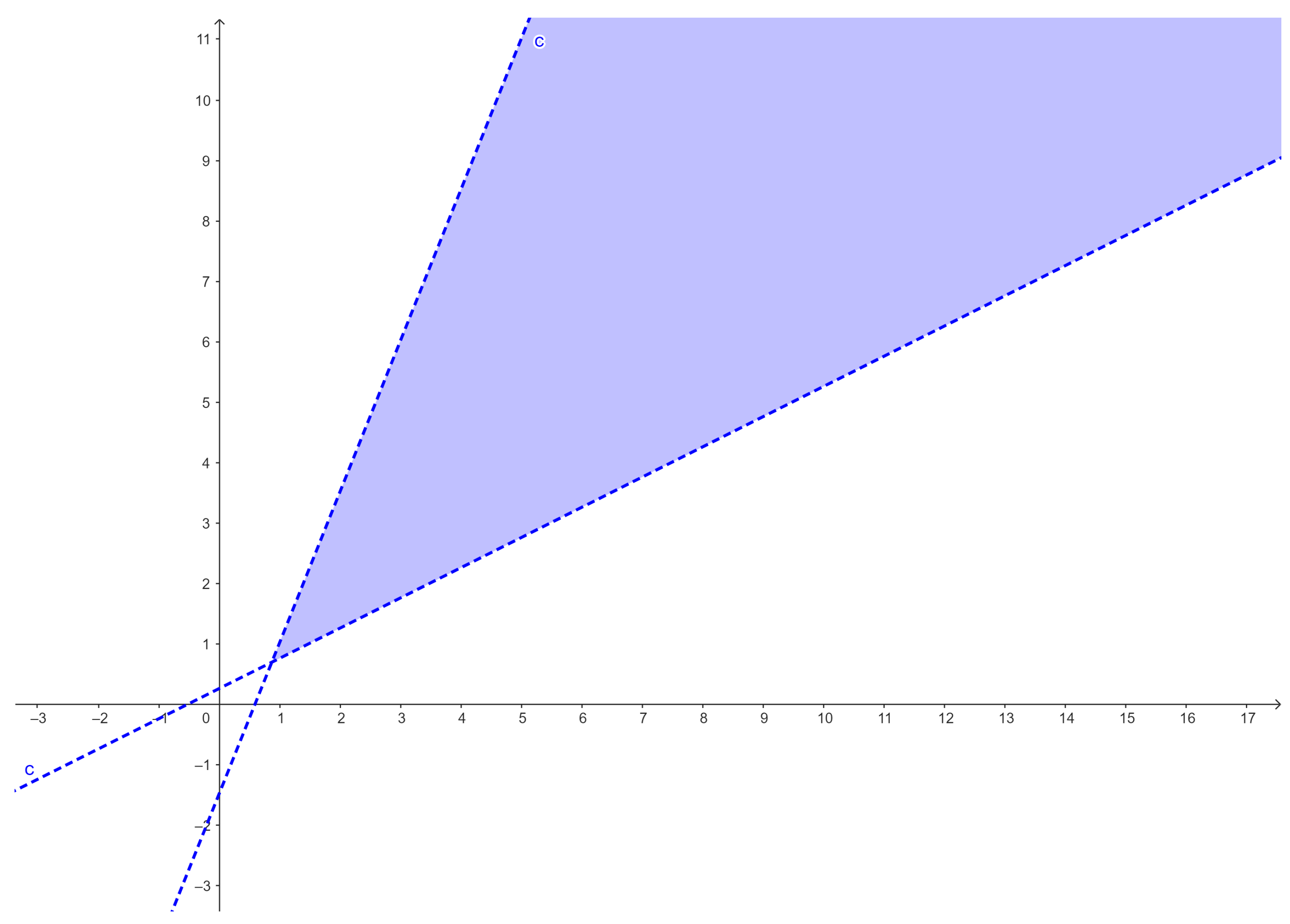
Figure 1 shows the region of points ( p , q ) calculated by GeoGebra Classic 6.0.794.0, where Condition (58) holds.
By Definition 2, the functions
γ 1 ( x ) , γ 2 ( x ) 0 , 0 , ϕ 1 ( x ) , ϕ 2 ( x ) p , q ,
are, respectively, the lower and upper solutions of Problems (56) and (57) for
μ p 3 5 p + 2 q , 0 , and λ q 1 + 2 p 4 q , 0 .
Moreover, Problems (56) and (57) are a particular case of (1) and (2), where
f ( x , y 1 , y 2 , y 3 ) = y 1 3 5 y 1 + 2 y 2 ,
and
g ( x , y 1 , y 2 , y 3 ) = y 2 1 + 2 y 1 4 y 2 .
These functions satisfy the Nagumo Conditions (7) and (8), relative to the intervals y 1 [ 0 , p ] and y 2 [ 0 , q ] as
| f ( x , y 1 , y 2 , y 3 ) | = y 1 3 5 y 1 + 2 y 2 p 3 5 p + 2 q : = φ 1 ( y 3 ) ,
| g ( x , y 1 , y 2 , y 3 ) | = y 2 1 + 2 y 1 4 y 2 q 1 + 2 p 4 q : = φ 2 ( y 3 ) ,
and, trivially,
0 + d s φ i ( s ) = + , for i = 1 , 2 .
Therefore, by Theorem 1, for the values of μ and λ fulfilling (59), Problems (56) and (57) have at least one solution ( u 1 ( x ) , u 2 ( x ) ) such that
0 u 1 ( x ) p , and 0 u 2 ( x ) q ,
for all x [ 0 , 1 ] .
Therefore, by Theorem 3, there are μ 0 > μ 1 and λ 0 > λ 1 such that Problems (56) and (57) have no solution for μ > μ 0 > 0 or λ > λ 0 > 0 and have at least one solution for
0 > μ μ 1 > p 3 5 p + 2 q , and 0 > λ λ 1 > q 1 + 2 p 4 q .

5.2. Interaction by Neutralism

Neutralism is an ecological relationship in which there is no interspecific interaction and the two species evolve independently, i.e., when both interaction parameters are null.
Consider in (54) ψ 1 = 0 and ψ 2 = 0 . Consider also the numerical Problems (56) and (57) with the same values for the other parameters:
u 1 ( x ) + u 1 ( x ) 3 5 u 1 ( x ) = μ cos 2 ( x ) , u 2 ( x ) + u 2 ( x ) 1 4 u 2 ( x ) = λ e x , x [ 0 , 1 ] ,
with boundary conditions
u i ( 0 ) = u i ( 1 ) = 0 , for i = 1 , 2 .
The assumptions (48) and (49) of Theorem 3 are satisfied for every x 0 , 1 , and the estimations of the parameters are given by
0 > μ 1 > p 3 5 p , when p > 3 5 ,
and
0 > λ 1 > q 1 4 q , when q > 1 4 .
Let 0 > ϵ 1 > 3 5 p and 0 > ϵ 2 > 1 4 q be real numbers. Then, the functions
γ 1 ( x ) , γ 2 ( x ) = ϵ 1 , ϵ 2 , ϕ 1 ( x ) , ϕ 2 ( x ) = p , q ,
are, respectively, strict lower and upper solutions of Problems (60) and (61) according to Definition 3 for
μ p ( 3 5 p ) , ϵ 1 ( 3 5 ϵ 1 ) , and λ q ( 1 4 q ) , ϵ 2 ( 1 4 ϵ 2 ) .
Moreover, Problems (60) and (61) are a particular case of (3) and (4), with
f ( x , y 1 , y 2 ) = y 1 3 5 y 1 ,
and
g ( x , y 1 , y 2 ) = y 1 1 4 y 1 .
These functions satisfy the Nagumo Conditions (7), and (8) relative to the intervals y 1 [ ϵ 1 , p ] and y 2 [ ϵ 2 , q ] as
| f ( x , y 1 , y 2 ) | = y 1 3 5 y 1 p 3 5 p : = φ 1 ¯ ( y 2 ) ,
| g ( x , y 1 , y 2 ) | = y 1 1 4 y 1 q 1 4 q : = φ 2 ¯ ( y 2 ) ,
and, trivially,
0 + d s φ i ¯ ( 2 ) = + , for i = 1 , 2 .
Thus, by Theorem 1, for the values of μ and λ fulfilling (62), Problems (60) and (61) have at least a solution ( u 1 ( x ) , u 2 ( x ) ) such that
ϵ 1 < u 1 ( x ) < p and ϵ 2 < u 2 ( x ) < q
for all x [ 0 , 1 ] .
By Theorem 3, there are μ 0 and λ 0 such that there is no solution if μ > μ 0 = 0 or λ > λ 0 = 0 .

6. Conclusions and Further Works

To the best of our knowledge, the present study represents the first time that sufficient conditions are given to apply the Ambrosetti–Prodi alternative to systems of differential equations with different parameters. The existence and non-existence of solutions are obtained for coupled systems, that is, for cases where there are strong relationships between the two unknown functions. However, the existence of multiple solutions was proved only for independent systems, that is, without the interaction of both variables. We underline that the assumptions rely only on local monotone assumptions about the nonlinearities and on the existence of a kind of bifurcation of the values of the parameters.
Several issues still remain open, justifying future work. For example:
  • In the coupled systems, what are the assumptions that are necessary to allow the nonlinearities to depend on the first derivatives of both variables?
  • How do we obtain the multiplicity result for the coupled system case?

Author Contributions

Formal analysis, F.M.; Investigation, F.M. and G.R.; Writing—original draft, G.R.; Writing—review & editing, F.M. All authors have read and agreed to the published version of the manuscript.

Funding

This research received no external funding.

Data Availability Statement

No new data were created.

Conflicts of Interest

The authors declare no conflict of interest.

References

  1. Ambrosetti, A.; Prodi, G. On the inversion of some differentiable mappings with singularities between Banach spaces. Ann. Mat. Pura Appl. 1972, 93, 231–246. [Google Scholar] [CrossRef]
  2. Fialho, J.; Minhós, F. Multiplicity and location results for second order functional boundary value problems. Dyn. Syst. Appl. 2014, 23, 453–464. [Google Scholar]
  3. Senkyrik, M. Existence of multiple solutions for a third-order three-point regular boundary value problem. Math. Bohem. 1994, 119, 113–121. [Google Scholar] [CrossRef]
  4. Chen, Q.; Li, J. Existence of Multiple Positive Solutions for Third-Order Three-Point Boundary Value Problem. J. Appl. Math. Phys. 2019, 7, 1463–1472. [Google Scholar] [CrossRef]
  5. Sovrano, E. Ambrosetti-Prodi type result to a Neumann problem via a topological approach. Discret. Contin. Dyn. Syst. S 2018, 11, 345–355. [Google Scholar] [CrossRef]
  6. Fabry, C.; Mawhin, J.; Nkashama, M. A Multiplicity Result for Periodic Solutions of Forced Nonlinear Second Order Ordinary Differential Equations. Bull. Lond. Math. Soc. 1986, 18, 173–180. [Google Scholar] [CrossRef]
  7. Feltrin, G.; Sovrano, E.; Zanolin, F. Periodic solutions to parameter-dependent equations with a ϕ-Laplacian type operator. Nonlinear Differ. Equ. Appl. 2019, 26, 26–38. [Google Scholar] [CrossRef]
  8. Mawhin, J. The periodic Ambrosetti-Prodi problem for nonlinear perturbations of the p-Laplacian. J. Eur. Math. Soc. 2006, 8, 375–388. [Google Scholar] [CrossRef]
  9. Minhós, F.; Oliveira, N. On periodic Ambrosetti-Prodi-type problems. AIMS Math. 2023, 8, 12986–12999. [Google Scholar] [CrossRef]
  10. Yu, X.; Lu, S. A singular periodic Ambrosetti-Prodi problem of Rayleigh equations without coercivity conditions. Commun. Contemp. Math. 2021, 24, 2150012. [Google Scholar] [CrossRef]
  11. Papageorgiou, N.S.; Rădulescu, V.D.; Zhang, J. Ambrosetti–Prodi problems for the Robin (p,q)-Laplacian. Nonlinear Anal. Real World Appl. 2022, 67, 103640. [Google Scholar] [CrossRef]
  12. Ding, L.; Sun, M.; Tian, R. A remark on the Ambrosetti-Prodi type problem. Appl. Math. Lett. 2021, 111, 106648. [Google Scholar] [CrossRef]
  13. Sovrano, E.; Zanolin, F. Ambrosetti-Prodi Periodic Problem Under Local Coercivity Conditions. Adv. Nonlinear Stud. 2018, 18, 169–182. [Google Scholar] [CrossRef]
  14. Fialho, J.; Minhós, F. Solvability of second-order coupled systems on the half-line. Lith. Math. J. 2019, 59, 198–212. [Google Scholar] [CrossRef]
  15. Minhós, F.; Sousa, R. Nonlinear Higher Order Differential and Integral Coupled Systems: Impulsive and Integral Equations on Bounded and Unbounded Domains. In Trends in Abstract and Applied Analysis; World Scientific: Singapore, 2022; Volume 10, 242p, ISBN 978-981-122-512-3. [Google Scholar]
  16. Sousa, R.; Minhós, F. Heteroclinic and homoclinic solutions for nonlinear second-order coupled systems with ϕ-Laplacians. Comput. Appl. Math. 2021, 40, 169. [Google Scholar] [CrossRef]
  17. Wang, A.; Sun, J.; Zettl, A. The classification of self-adjoint boundary conditions: Separated, coupled. J. Funct. Anal. 2008, 255, 1554–1573. [Google Scholar] [CrossRef]
  18. Amann, H. Parabolic evolution and nonlinear boundary conditions. J. Differ. Equ. 1988, 72, 201–269. [Google Scholar] [CrossRef]
  19. Aronson, D.G. A comparison method for stability analysis of nonlinear parabolic problems. SIAM Rev. 1978, 20, 245–264. [Google Scholar] [CrossRef]
  20. Leung, A. A semilinear reaction-diffusion prey-predator system with nonlinear coupled boundary conditions: Equilibrium and Stability. Indiana Univ. Math. J. 1982, 31, 223–241. [Google Scholar] [CrossRef]
  21. Mehmeti, F.A.; Nicaise, S. Nonlinear interaction problems. Nonlinear Anal. 1993, 20, 27–61. [Google Scholar] [CrossRef]
  22. Minhós, F.; Carapau, F.; Rodrigues, G. Coupled systems with Ambrosetti-Prodi-type differential equations. AIMS Math. 2023, 8, 19049–19066. [Google Scholar] [CrossRef]
  23. Nagumo, M. Über die diferencialgleichung y” = f (x, y, y’). Proc. Phys. Math. Soc. Jpn. 1937, 364, 861–866. [Google Scholar]
  24. Andreguetto Maciel, G.; Martinez-Garcia, R. Enhanced species coexistence in Lotka-Volterra competition models due to nonlocal 366 interactions. J. Theor. Biol. 2021, 530, 110872. [Google Scholar] [CrossRef] [PubMed]
  25. Al Noufaey, K.; Marchant, T.; Edwards, M. The diffusive Lotka–Volterra predator-prey system with delay. Math. Biosci. 2015, 270, 30–40. [Google Scholar] [CrossRef] [PubMed]
  26. Wang, Q. Qualitative analysis of a Lotka–Volterra predator–prey system with migration. J. Math. Anal. Appl. 2019, 472, 421–431. [Google Scholar] [CrossRef]
Figure 1. Region of points ( p , q ) .
Mathematics 11 03645 g001
Disclaimer/Publisher’s Note: The statements, opinions and data contained in all publications are solely those of the individual author(s) and contributor(s) and not of MDPI and/or the editor(s). MDPI and/or the editor(s) disclaim responsibility for any injury to people or property resulting from any ideas, methods, instructions or products referred to in the content.

