1. Introduction
Traffic congestion is an unprecedented problem in many major cities in the United States. The number of vehicles on road has increased significantly in recent years, leading to increased congestion. In year 2021, there were an estimated 282 million registered vehicles in the United States, up from 225 million in year 2000 [
1]. According to data from the Census Bureau [
2], there were about 1.8 vehicles available per US household in year 2016. These number of vehicles per household varies depending on the city and its population density. For example, in Austin, Texas, the population in year 2016 was 925 K [
3] and there were 1.9 vehicles per household in year 2016 [
2].
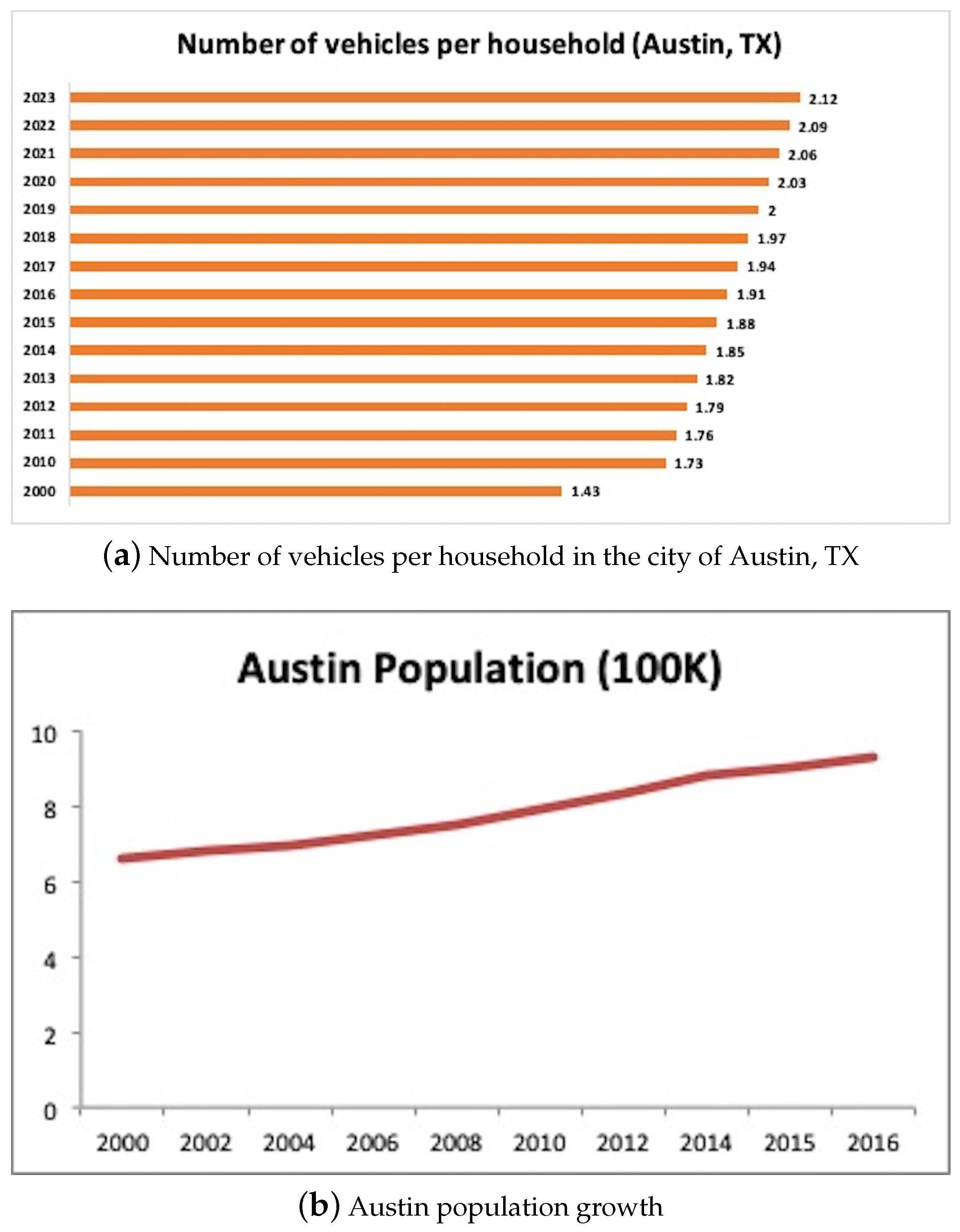
Figure 1a,b show that the number of vehicles per household and population density in Austin has been steadily increasing in recent years [
1,
3]. In year 2000, the average number of vehicles per household in Austin was 1.43. This number has increased by 48.2% in the past 23 years, up to 2.12 in year 2023. On the other hand, the population in Austin is also expected to increase by at least 30% by year 2030 [
4]. This will lead to an even greater increase in the number of vehicles on road, and will further exacerbate the problem of traffic congestion. According to an INRIX report [
5] and a congestion statistics report [
6], due to poor traffic conditions, Austin-area commuters wasted about 41 h on average in traffic in year 2020 (3 hours more than in year 2012), the seventh-highest of any city in the country, thereby increasing the overall travel time by 22%. The problem of traffic congestion is expected to worsen due to future predicted population growth, which can lead to significant increase in travel times, decreased fuel efficiency, and increased air pollution. It can also have a negative impact on businesses and city’s economy. One way to alleviate traffic congestion is to use efficient routing strategies. These strategies can help drivers find the fastest and most efficient routes to their destinations, and help drivers avoid congested areas.
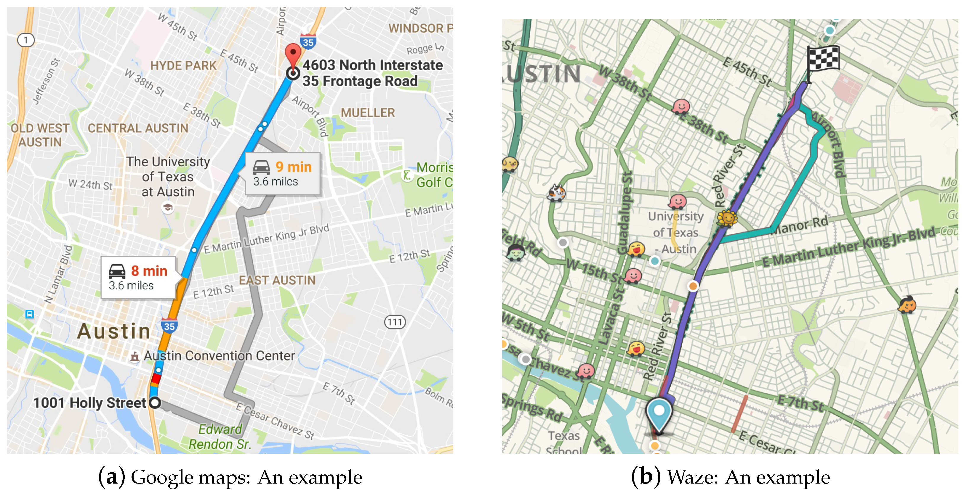
There are various strategies and tools currently available to develop optimized routes. For example, Google Maps and Waze route in different ways and serve a different clientele. Google Maps creates a fixed static route which is easier to navigate but could be potentially slow. On the other extreme, Waze provides an aggressive adaptive route. A snapshot of routes generated between a specific source–destination pair using Google Maps and Waze are shown in
Figure 2a and
Figure 2b, respectively. It is to be noted that the latter recommends a recourse path en route to the destination, which is depcited in
Figure 2b with teal color. An (aggressive) adaptive route by Waze is a potentially faster route that dynamically changes and adapts to traffic conditions, but the frequent route changes may lead to high stress in navigation. To alleviate this issue and create a middle-ground that seeks the best of both extremes, in this work, we develop a methodology to compute non-aggressive adaptive routes.
A non-aggressive adaptive route adapts dynamically to changing traffic conditions but in a limited way—for example, by allowing only a certain number of route-shifts at critical junctures. These routes seek to provide both low travel times and low stress of navigation. At the start of the route, the conditions on the roads are only known through a probability distribution. As the driver approaches closer to individual intersections, specific road conditions are observed and the routes are adjusted to minimize the travel time.
The contributions of this paper can be summarized as follows:
We propose a novel routing framework for routing in road networks with limited adaptability. We call this non-aggressive adaptive routing, aiming to seek both low travel times and low navigation stress compared to traditional routing technologies like Google Maps and Waze;
We design several strategies to model and compute such non-aggressive adaptive routes, based on where and how the route adjustments are performed;
We develop exact mathematical methods such as complete enumeration and dynamic programming algorithms for each of the strategies. We also derive easily computable bounds that can be used to solve these algorithms efficiently for large networks;
We evaluate and analyze the performance of proposed algorithms using the Austin road network as an example and demonstrate the benefits of limited adaptability.
The remainder of the paper is organized as follows. In
Section 2, we discuss the related work on adaptive routing. In
Section 3, we present our proposed routing strategies and the respective solution methodologies. In
Section 4, we develop efficient bounds to render our algorithms tractable for large sized networks, and also present the computational evaluation of our proposed tractable algorithms using Austin road network. Finally,
Section 5 concludes our work by summarizing the key contributions and pointing to future research directions.
2. Related Work
Consider the case of routing a driver from point
s to
t in a traffic network. Adaptive routing is a stochastic shortest path problem where the edge costs are unknown until arriving at one of its endpoints. The decision to continue or change the route is based on the traffic condition at that edge. Croucher [
7] appears to be the first to have studied a model of this type but in a fairly restricted setting. In that model, a first-choice arc is selected for every node, there is some probability that the arc fails, and, if it fails, a second outgoing arc is selected at random. Andretta and Romeo [
8] considered a similar model with the choice of recourse computed in an optimal way. In their work, a recourse path to the destination is computed for every edge, assuming that the edge is inactive. In our work, if an edge has traffic congestion, it is still considered active with greater time delay for traversal. Additionally, if an edge is selected for observation and found to be congested, the driver may revert to a recourse route. Unlike the past literature, our work describes a sequence of models in which the driver may observe between one and all edges for traffic congestion.
Another widely studied variant of adaptive routing is the Canadian Traveller Problem (CTP). CTP was first defined in [
9] (see also [
10]). The goal is to find an optimal routing policy that guarantees a good route under uncertain road conditions, minimizing the expected cost of travel. In this problem, the arc costs are deterministic but unknown and, once a road is considered blocked, it remains blocked forever. In general, CTP is known to be #P-hard and there has been no significant progress on approximation algorithms. Several variants to this problem, such as
CTP,
vital edges problem, and deterministic and stochastic recoverable CTP, are defined in [
11]. Polychronopoulos and Tsitsiklis [
12] presented another variation to CTP where the realization of arc costs is learned progressively as the graph is traversed. They provided dynamic programming algorithms to solve models with both dependent and independent arc costs and they established that the running time of these algorithms is exponential in number of arcs. There are few other algorithms that address the adaptive routing problem with time-dependent and stochastic costs [
13,
14,
15,
16]. In our work, we assume independent arc costs and limit the number of re-routing decisions, as opposed to CTP and its variants. We also present tractable dynamic programming algorithms which are solvable in polynomial time.
Special cases of CTP were studied by Nikolova and Karger [
17] to explore exact solutions. They explained the connection of CTP to Markov Decision Processes (MDPs) solvable in polynomial time. They also presented polynomially solvable dynamic programming algorithms for a standard version of CTP on directed acyclic graphs (DAGs). It is important to note that our problem is a generic version of CTP. CTP can be derived by equating the number of re-routing decisions to the total number of edges in the network, which, in one of our proposed routing strategies, we call the
parallel model.
The research presented here complements these works by examining non-aggressive adaptive routing, identifying an optimal yet small number of decision points on a route. The focus of our work is to derive the benefits of adaptive routing but with a limited number of adaptations to reduce driving stress. To this end, we propose, compare, and contrast several models for defining the decision points, and develop tractable algorithms to compute the optimal routing policy.
Many other recent extensions to adaptive routing have been proposed, primarily focusing on route planning under uncertainty for different modes of transportation [
18,
19,
20], route planning under uncertainty with optimal information location points [
21], stability of transportation networks [
22], stochastic time-dependent networks [
23], maximizing the probability of on-time arrival [
24], application to online decision problems [
25], and competitive analysis of CTP [
26].
Another emerging field in adaptive routing models is the development of connected automated vehicles (CAV) technology [
27,
28], vehicle-to-vehicle (V2V) commnuication [
29], and automonous vehicle tracking [
30,
31], with a variation to consider user preferences [
32]. CAVs can provide real-time information about the individual position and velocity of vehicles, which can be used to develop more accurate and efficient routing algorithms. However, in this work, we focus on macroscopic routing models with high-level traffic congestion and delay information. We believe that, by understanding macroscopic traffic patterns, we can develop better routing algorithms for both CAVs and non-CAVs in the future.
3. Model Description
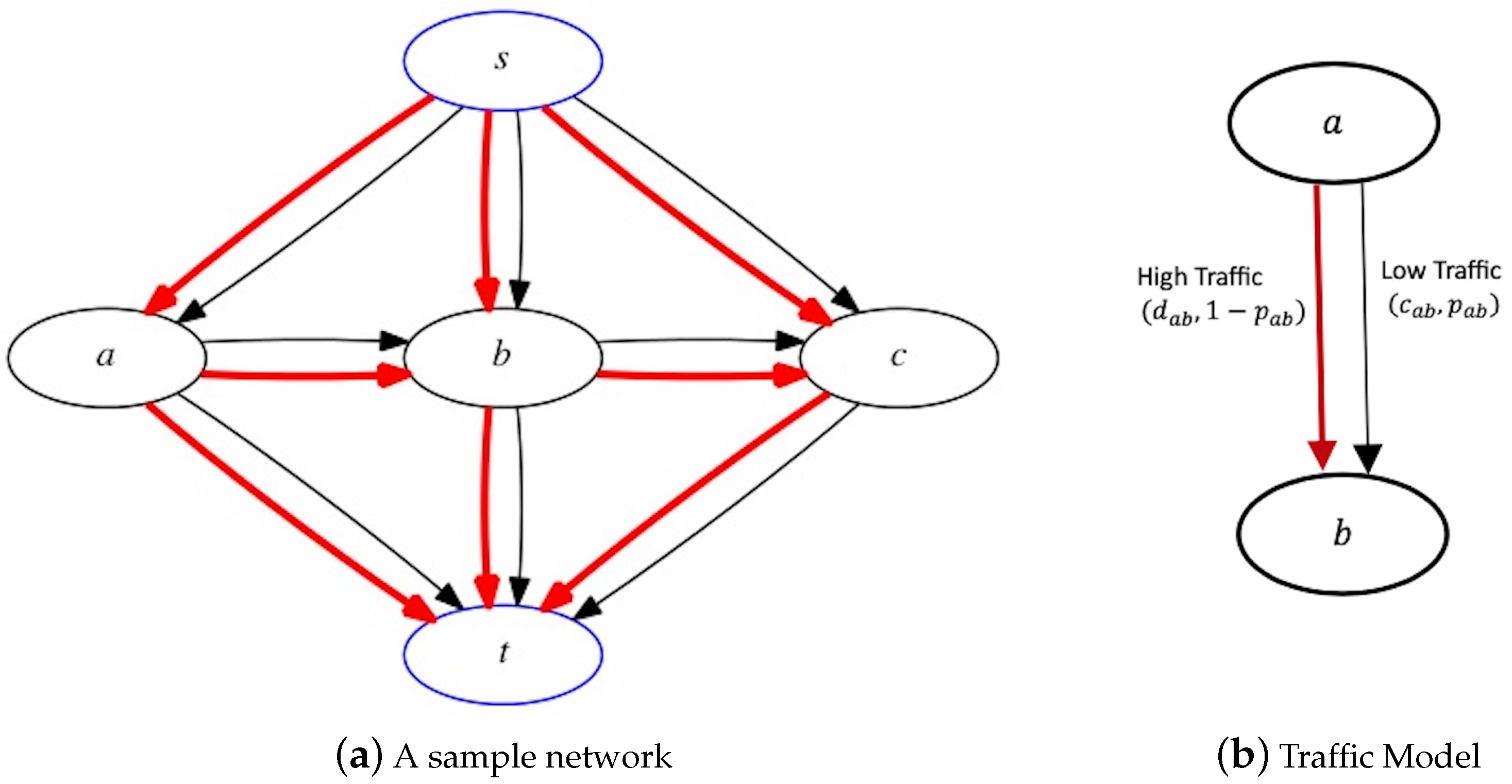
Consider a directed acyclic network
, with specified source
s and destination
t nodes, as shown in
Figure 3a. We believe that directed acyclic networks (DAGs) are a more general representation of real-world traffic networks and best suited to generate practical recommendations to users. On a city road network
G,
N represents the set of road intersections and
A represents the set of roads or edges connecting those intersections. We consider potential traffic congestion on the edges given by the set
A.
We examine a simple model of traffic congestion where each edge is in either a high traffic state or low traffic state, independently of other edges. The traffic probability distribution is assumed to be known ahead of time. Every edge
is defined by three inputs:
, where
represents the travel time under low traffic,
represents the travel time due to high traffic, and
represents the probability of low traffic on the edge. This is visually depicted in
Figure 3b.
Given these inputs, we determine the edges to be observed for traffic congestion and the corresponding adjustment routes should high traffic states be observed on those edges. We call an edge selected for observation and for possible route adjustment an adjustment edge. When the driver reaches the source node of an adjustment edge and observes low traffic, they proceed through the edge. If the driver observes high traffic, then they take an adjustment route. To simplify the exposition, we start with a single route adjustment and then provide several extensions to multiple route adjustments. A detailed discussion on these route adjustment strategies is presented in the following subsections.
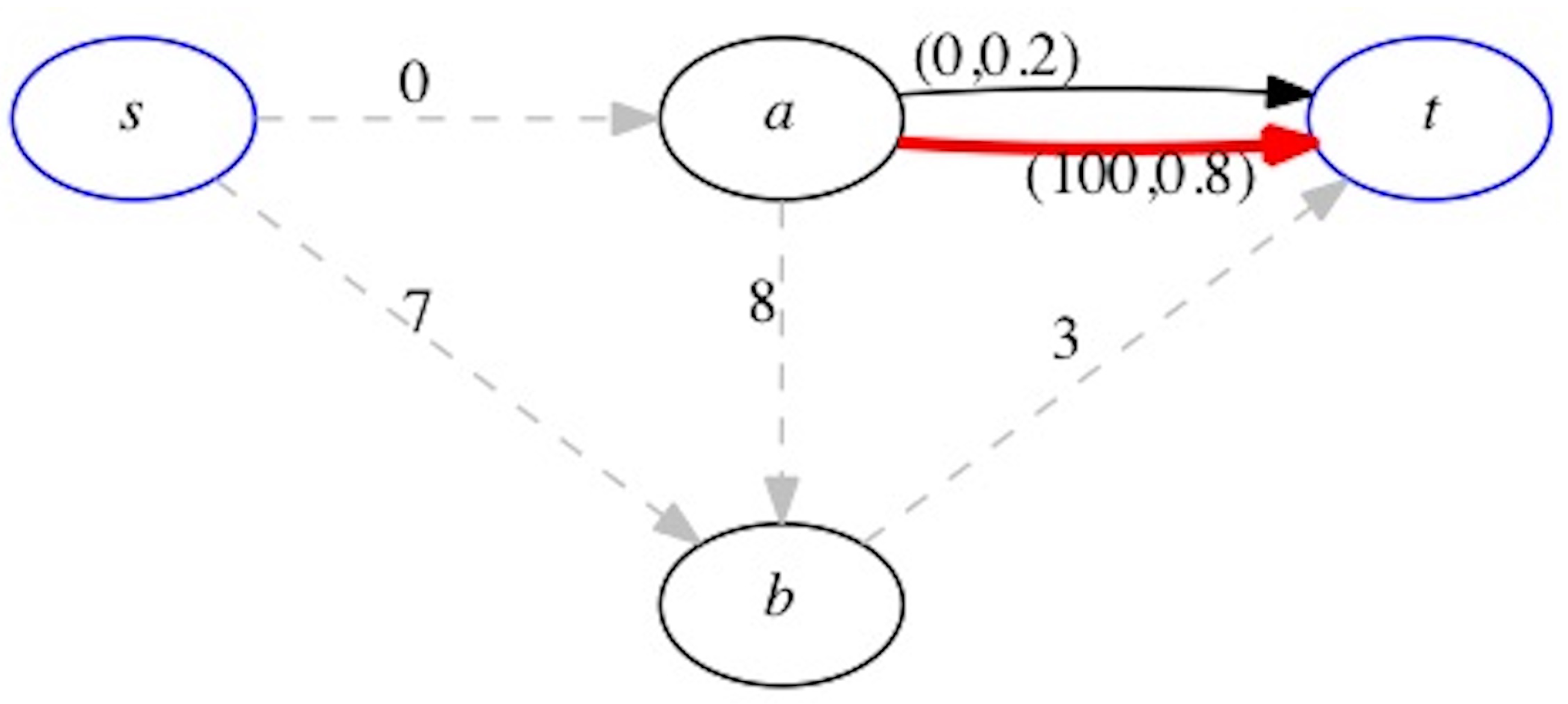
We begin with a simple example presented in
Figure 4. This example shows that the optimal adjustment edge need not be a part of the fixed non-adaptive shortest route. The shortest path from
s to
t can be computed as
with expected travel time 10. If edge
is observed, there is 20% chance of low traffic with zero travel time. However, there is 80% chance of high traffic at edge
, and, if the driver adjusts the route to
, then the travel time is 11. With the single observation of edge
, the expected travel time is
, which is lower than the expected travel time without any adjustments (which is equal to 10). An interesting aspect of this example is that the edge
is not on the fixed (no-adjustment) shortest path.
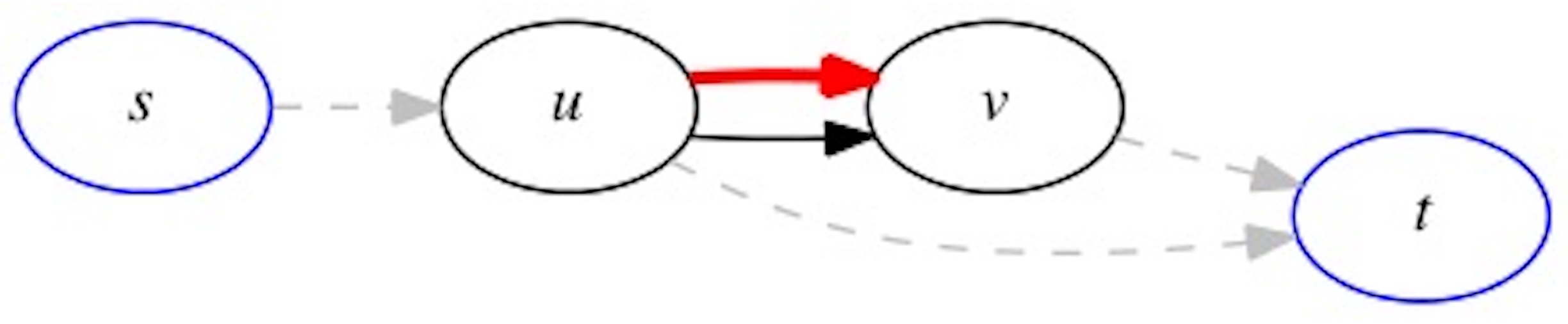
3.1. Single Route Adjustment Policy
A pictorial representation of a single route adjustment policy is shown in
Figure 5, where the route from source
s to destination
t has a single adjustment edge,
. In this policy, the driver takes the shortest path from
s to
u, and observes edge
for traffic. In case of low traffic, driver continues on the edge
and takes the shortest path from
v to
t. In case of high traffic, driver takes an adjustment route from
u to
t. The overall expected travel time for any adjustment edge
is computed using
where
represents the expected travel time of a no-adjustment shortest path from node
i to
j,
represents the expected travel time of a no-adjustment shortest path given edge
is congested, and
represents the expected travel time of a single route adjustment policy using the adjustment edge
. One could determine the adjustment edge that yields minimal expected travel time,
, using complete enumeration, given by
where
represents the overall minimum expected travel time from
s to
t due to the single-route adjustment policy. An equivalent integer programming formulation is presented in
Appendix A.1.
3.2. Multiple Route Adjustment Policy
There are several potential models for multiple route adjustments. We present and explore three different strategies that we call the series unforced, series forced, and parallel models. We develop dynamic programming-based algorithms to solve these route adjustment models, and, finally, compare their performances.
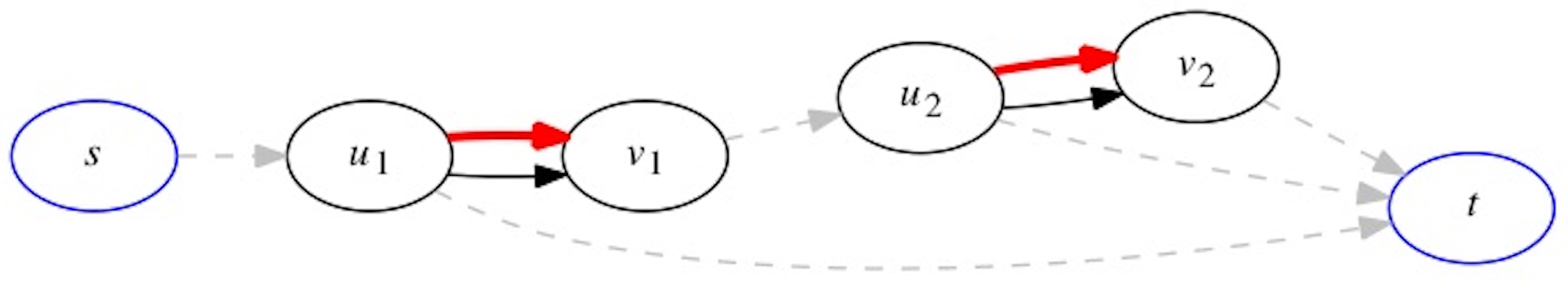
3.2.1. Series Unforced Model
Let us start with two adjustment edges as shown in
Figure 6, which follow what we call a
series unforced model. In this model, once the driver makes a route adjustment, he loses the potential to observe the other edges for traffic. Say, for instance, the source
s and destination
t nodes are connected by a highway. The driver enters the highway from source
s, and, upon arriving at
, observes edge
for traffic. In case of high traffic, driver adjusts the route to reach the destination
t and never gets to make any other route adjustments. In case of low traffic, driver traverses the edge
, and continues on the highway until
where they observe edge
for traffic. In case of high traffic at
, driver adjusts the route to destination
t. In case of low traffic, driver traverses the edge
, and continues on the highway to reach the destination
t.
Let
denote the expected travel time with respect to the adjustment edges
and
. One could find a pair of edges that yield a minimum expected travel time through complete enumeration,
, using
The first summand is the expected travel time from
s to
. The second summand is the expected travel time from
to
t if high traffic is observed at
. The third summand is the travel time from
to
t if low traffic is observed at
. This third summand includes within it a version of (
1), computing the travel time from
to
t that is dependent on the observation of traffic at edge
. Similarly, one could express the computation of the minimum expected travel time with
k adjustment edges recursively with the equation for
adjustment edges as follows. Let
denote the overall minimum expected travel time when
k adjustment edges are observed for traffic. We can then write
The basecase
represents the minimum expected travel time for a single adjustment edge. The recursive equation to compute
includes a
in case it is unnecessary to observe
k edges. The second term involves picking the first edge
for observation, and the remaining length of the paths to destination is based on the probabilities of that observation.
The recursive Equation (
4) yields a dynamic programming algorithm for computing the best set of
k adjustment edges. The dynamic programming algorithm reduces the computational effort from
, roughly what is required with complete enumeration using (
3), to
, where
. This brings significant computational savings, though, as is discussed later, this is still insufficient for practical applications.
3.2.2. Series Forced Model
An alternate model with two adjustment edges, which we call
series forced, is depicted in
Figure 7. In this model, the driver is forced to observe all the adjustment edges; hence, they have the potential to adjust the route at every such adjustment edge. Consider the same instance where the driver enters the highway from source
s and observes an edge
for traffic. In case of high traffic, driver adjusts the route but returns to the next source node
to observe adjustment edge
. In case of low traffic, driver traverses the edge
, and continues on the highway until
, where they observe edge
for traffic. In case of high traffic at
, driver adjusts the route to destination
t. In case of low traffic, driver traverses the edge
, and continues on the highway to reach the destination
t. In this model, the driver always observes all the adjustment edges, irrespective of the traffic states of previous adjustment edges.
Let
denote the expected travel time if adjustment edges
and
are selected. One could find a pair of adjustment edges that yield a minimum expected travel time, which is given by
through complete enumeration using
The first summand in (
5) is the expected travel time from
s to
. This first summand includes within it a version of (
1), computing the travel time from
s to
as dependent on the observation of edge
. The second summand is the expected travel time from
to
t with traffic state observed at
. Thus, (
5) can be expressed as a recursive equation for
k adjustment edges as follows:
where
denotes the overall minimum expected travel time obtained using the series forced model when
k adjustment edges are observed for traffic. Though inefficient, an integer programming formulation for this model is presented in
Appendix A.2.
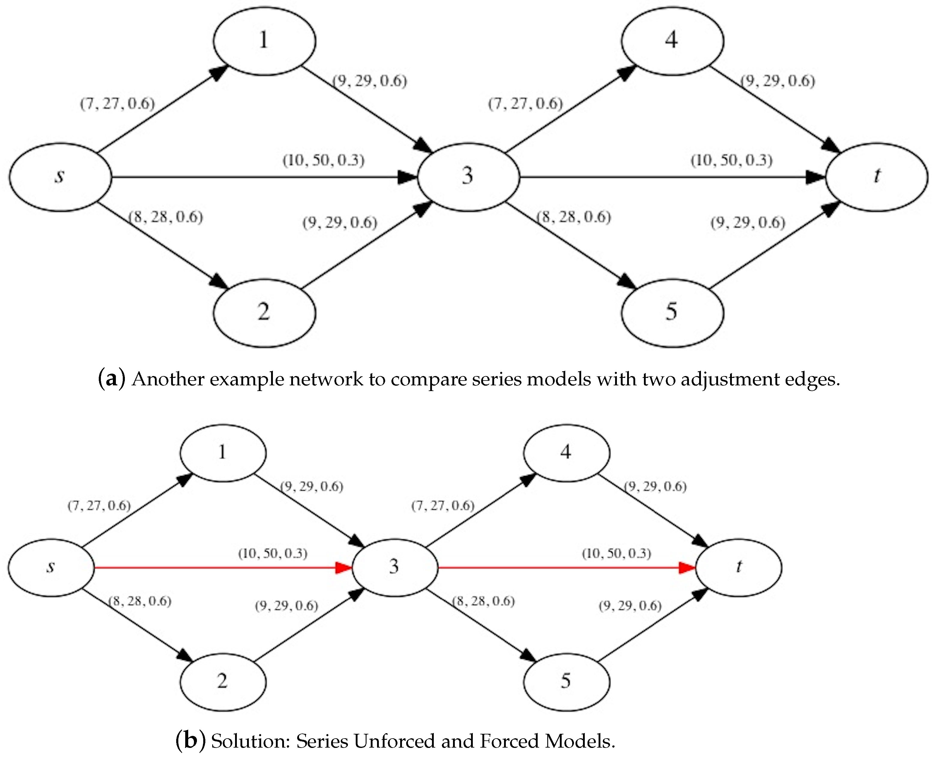
An interesting fact is that there is no evidence to show the superiority of one series model over the other, in terms of reducing expected travel time. To illustrate this, let us consider the example network in
Figure 8a. The edge weights
represent the travel time under low traffic, the travel time under high traffic, and the probability of low traffic, respectively. The expected travel time of the series models are computed using (
4) and (
6), and the resulting best adjustment edges are highlighted in red in
Figure 8b and
Figure 8c, respectively. We obtain
as 34.8 and
as 35.6, with the series unforced model performing better than the series forced model. Let us now consider another example network as in
Figure 9a. We follow the same routine to obtain
as 55.4 and
as 50.8. In this network, the series forced model performs better than the series unforced model. This shows that the performances of the series models are incomparable, and they depend on the network instance considered. Generally, one may think that the series forced model should perform better, because it has the ability to execute several observations in sequence as opposed to just one. However, as these examples demonstrate, it may be too expensive to execute the secondary observations, when unnecessary, as compared to the series unforced model.
3.2.3. Parallel Model
Another model with two adjustment edges, which we call
parallel, is depicted in
Figure 10. In this model, the driver has the potential to observe edges and make route adjustments, in both original and adjustment routes. Consider the same instance where the driver enters the highway from source
s and observes an edge
for traffic. In case of low traffic, driver traverses the edge
, and continues on the highway until
, where they observe edge
for traffic. In case of high traffic at
, driver adjusts the route to reach node
and observes an edge
for traffic in the adjusted route. In case of high traffic at the second adjustment edge (
or
), driver adjusts the route to destination
t. In case of low traffic, driver traverses the edge, and continues on the route to reach the destination
t. Unlike series models, here driver observes different adjustment edges based on the traffic state of previous adjustment edges.
Let
denote the expected travel time if adjustment edges
,
, and
are selected. One could find a set of adjustment edges that yield a minimum expected travel time,
,
,
, through complete enumeration using
The first summand is the expected travel time from
s to
. The second and third summands together represent the weighted sum of expected travel times from
to
t, with weights representing the traffic state at
. The second summand includes within it a version of (
1), computing the travel time from
to
t as dependent on the observation of edge
. The third summand includes within it a modified version of (
1), the difference being the first term, where we compute the expected travel time from
to
given that high traffic is observed at
.
Let
denote the overall minimum expected travel time from
s to
t with
k adjustment edges. It is to be noted that the driver’s policy may include more than
k adjustment edges, but only
k edges will be observed in total as they travel from
s to
t. We now express (
7) as recursive equations as follows:
where
denotes the minimum expected travel time from any
g to
i, given that high traffic is observed at all edges in set
.
It is easy to see that the series models are special cases of parallel model, i.e., a solution to a series model can be expressed as a solution to the corresponding parallel model. Hence, the parallel model always outperforms the series models in terms of reducing travel time, but at the expense of more computational effort. It also follows that a parallel model reduces to a Canadian Traveller Problem (CTP) on directed acyclic graphs (DAGs) when all edges in the network are observed for traffic, i.e.,
k equals
. Thus, the proposed dynamic programming algorithm can be used to solve CTP on DAGs. The dynamic programming algorithm proposed in [
17] differs from our algorithm mainly by the following two points:
- (1)
In [
17], an optimal outgoing edge is computed upon arrival at a node as the graph is traversed. This is different from our dynamic programming approach, where we pre-compute both the original and adjustment routes to the destination;
- (2)
The algorithm [
17] iterates over all the edges in the network, whereas our algorithm is made to stop when observing more adjustment edges no longer reduces the expected travel time.
4. Large Scale Tractable Algorithms
We use the Austin road network (
Figure 11) to evaluate the performance of our proposed dynamic programming algorithms. The travel times
c on the edges are known (Source URL:
http://austintexas.gov/department/gis-and-maps/gis-data, accessed on 2 November 2018), and we assume the probability of low traffic and delay offsets based on the street type, as depicted in
Figure 11. The Austin road network consists of about 100,000 edges and it is impractical to find the best adjustment edges, even in a single route adjustment policy, through complete enumeration. For example, it takes about 6 h to find a single adjustment edge for the example source–destination pair shown in
Figure 11. Inspired by the traditional branch and bound techniques, we develop easily computable lower and upper bounds to first prune the network and then eliminate many possibilities of adjustment edges, in order to reduce the overall problem size and create truly tractable algorithms.
4.1. Network Pruning
We first focus on developing some easily computable upper and lower bounds to prune the network size. This improves the run time of the shortest path procedures and, consequently, the tractability of the proposed dynamic programming algorithms.
Let represent the minimum expected travel time with k adjustment edges and any route adjustment model .
Lemma 1. The minimum expected travel time between two nodes s and t is non-decreasing with k adjustment edges, i.e., .
Proof. The recursive Equation (
8) shows that
, for any
. Recursively, we can write,
. To show
, consider an edge
on the shortest path from
s to
t. Then, the expected travel time of the shortest path,
, can be written as
A term-by-term comparison of (
9) with (
1) shows that
is an upper bound to
because going through a high traffic edge
is one potential routing for
. Thus,
is an upper bound to
. Using similar logic, the lemma can be proven for the series models as well. □
Let us assume that there exists an optimal policy
that includes edge
on one of the paths generated and let
be the corresponding expected travel time. A lower bound on the travel time of any path going through edge
can be given by
where
represents the shortest path from
i to
j with edge lengths
c, i.e., assuming low traffic on all the edges.
Let . In other words, the probabilities of low traffic are bounded away from (0, 1) by at least . Under a single route adjustment, every path occurs in policy with probability of at least . Under k route adjustments, every path occurs with probability of at least . This leads to the following lemma defining a lower bound on any policy that uses edge .
Lemma 2. Every k-route adjustment policy π that includes edge on some path has .
Proof. Any path with edge occurs with probability at least and has length at least . All other paths in the policy have length at least . □
Now, we are ready to present our theorem on network pruning.
Theorem 1. An edge with , for any , will not be on any path in the optimal routing policy.
Proof. Let denote the optimal routing policy. By Lemma 2, we have . If , by Lemma 1, is not an optimal routing policy. Hence, the edge will not be on any path in the optimal policy . □
Using the result of Theorem 1, one can prune the network by eliminating several possibilities. The network pruning procedure is also summarized in Algorithm 1. For the example source-destination pair considered, and for
and
, the network is pruned to 17,328 edges.
| Algorithm 1 Network Pruning |
- Require:
The following are input parameters: - 1.
which denotes city network with latitutde and longitude of nodes, and edges connecting those nodes; - 2.
Edge weights include free flow times , low traffic probability and travel time due to high traffic ; - 3.
Latitude and longitude of source s and destination t, and maximum number of adjustment edges k. - Ensure:
- 1:
function : - 2:
Create an empty network, - 3:
Compute the expected travel time due to shortest path from s to t as - 4:
for every edge do - 5:
Compute lower bound , using ( 10) and Lemma 2 - 6:
if then - 7:
Append edge to - 8:
end if - 9:
end for - 10:
return
|
4.2. Critical Adjustment Edges
In addition to pruning the network size, it is also possible to obtain a set of critical adjustment edges that contain the optimal solution (as summarized in Algorithm 2). For this, we employed different lower bounds, as discussed in this section.
Lemma 3. An optimal single route adjustment policy π with adjustment edge has , where is given by Proof. By definition, we have
. Edge
is an optimal adjustment edge, so using (
1) and (
2) yields
We proceed to complete the proof by contradiction.
Assume . Consider a policy that uses no adjustment edge and the route is followed by . Thus, the policy has length , implying is not optimal. This yields .
Using this result, we have
□
We define the following variables to simplify our notations in the remainder of the section. One can easily pre-compute these quantities and use it in subsequent computations.
Lemma 4. (Series unforced model)
. An optimal route adjustment policy π with edge as its first adjustment edge has , where , is given by Proof. Because
is an optimal policy and edge
is the first adjustment edge, using (
4), we have
We show , by contradiction. Assume . Consider a policy that uses no adjustment edges and the route is followed by . Thus, the policy has length , implying is not optimal. Thus, .
Using this result, we have
This is a valid yet intractable lower bound to
. To alleviate this issue, we derive a lower bound for
. The potential savings in travel time from
i to
j due to the single-route adjustment policy (using (
1) and (
4)) are given by
It is important to note that (
14) holds for all route adjustment models since
.
The potential savings in travel time from
i to
j due to the two-route adjustment policy are given by
The penultimate inequality is due to (
14). Combining this result with (
13) for
, we obtain
Extending this logic to any
k yields
□
Lemma 5. (Series forced model)
. An optimal route adjustment policy π with edge as its last adjustment edge has , where is given by Proof. Because
is an optimal policy and edge
is the last adjustment edge, using (
6), we have
Given edge is the optimal adjustment edge, we show following the same procedure as in the proof of Lemma 4.
Assume . Consider a policy that uses only the first adjustment edges of in the same sequence and does not use the last adjustment edge. In other words, the route is followed by . Thus, the policy has length , implying is not optimal. Thus, , given is the last adjustment edge.
Using this result, we have
We now proceed to obtain a tractable lower bound on
. The potential savings in travel time from
i to
j due to the two-route adjustment policy using (
6) are given by
The penultimate inequality is due to (
14). Combining this result with (
16) for
yields
By extending the logic to a generic
k, we obtain
□
Lemma 6. (Parallel model)
. An optimal route adjustment policy π with edge as its first adjustment edge has and , where is given by Proof. Because
is an optimal policy and edge
is the first adjustment edge, using (
8), we have
We show by contradiction. Assume . Consider a policy that uses the adjustment edges of the first adjusted route of (in the same sequence) and does not use any other adjustment edges. In other words, route is followed by . Thus, the policy has length , implying is not optimal. Thus, .
Using this result, we have
We follow the same procedure as in the proofs of Lemmas 4 and 5 to obtain a lower bound on
. The potential savings in travel time from
i to
j due to the two-route adjustment policy using (
8) are given by
The penultimate inequality is due to the fact that
and due to (
14).
Similarly, the potential savings in travel time from
i to
j due to the three-route adjustment policy are given by
The penultimate inequality is due to
and
. Using the above results in (
18) for
, we obtain
By similar logic, we derive, for any
k,
Since by definition, is a valid lower bound to . □
Now, we present our theorem to obtain a set of feasible adjustment edges.
Theorem 2. An edge with or cannot be the first adjustment edge (for M being series unforced or parallel models) or the last adjustment edge (for M being series forced model) in an optimal routing policy.
Proof. Let be a routing policy using series unforced model and edge as the first adjustment edge.
We show that is not optimal if .
If is optimal, we have , using the result of Lemma 4. Since (by assumption), we have , implying is not optimal. This completes our proof. Similar logic can be used along with Lemmas 5 and 6 to prove this claim for the series forced and parallel route adjustment models. □
| Algorithm 2 Critial Adjustment Edges |
- Require:
The following are input parameters: - 1.
A road network with edge weights , depicting free flow times , low traffic probability and travel time due to high traffic ; - 2.
Source s, destination t and number of adjustment edges k; - 3.
Routing model type , where ; and - 4.
Optimal expected travel time for route adjustment policy . Here, recursive term , from Algorithm 3 with respect to routing model and adjustment edges. - Ensure:
Set - 1:
function : - 2:
Create an empty set - 3:
if (Single route adjustment policy) then - 4:
for every edge do - 5:
Compute lower bound , as in Lemma 3 - 6:
if then - 7:
Append edge to set - 8:
end if - 9:
end for - 10:
end if - 11:
if , Multiple route adjustment policy then - 12:
for every edge do - 13:
Compute lower bound : (a) If model is Series Unforced Model, , as in Lemma 4 using ( 11) and ( 12) (b) If model is Series Forced Model, , as in Lemma 5 using ( 11) and ( 15) (c) If model is Parallel Model, , as in Lemma 6 using ( 11) and ( 17) - 14:
if then - 15:
Append edge to set - 16:
end if - 17:
end for - 18:
end if - 19:
return
|
These two pre-processing algorithms for pruning the network size and eliminating the possibilities of adjustment edges reduce the computation time from several hours to seconds. Specifically, it takes about 10 s to prune the network from 108,000 edges to 17,328 edges and to find a set of 21 feasible edges for a single route adjustment policy, which is depicted in
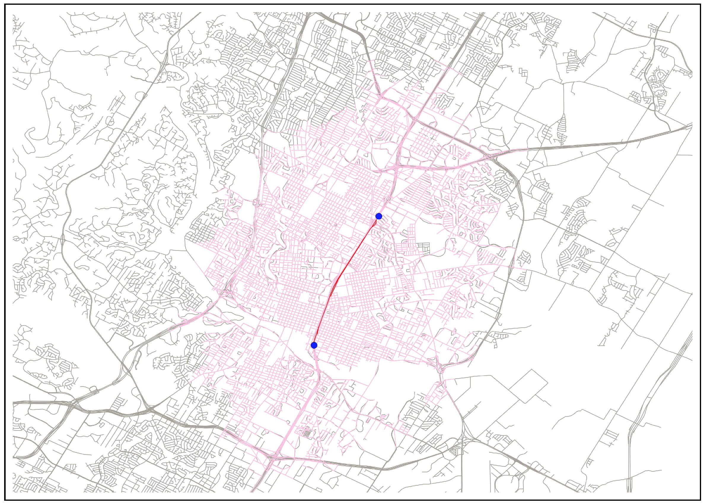
Figure 12. As a result of these pruning processes, the algorithm is able to compute an optimal single-route adjustment policy in less than 15 s. The solution pertaining to the example considered is presented in
Figure 13.
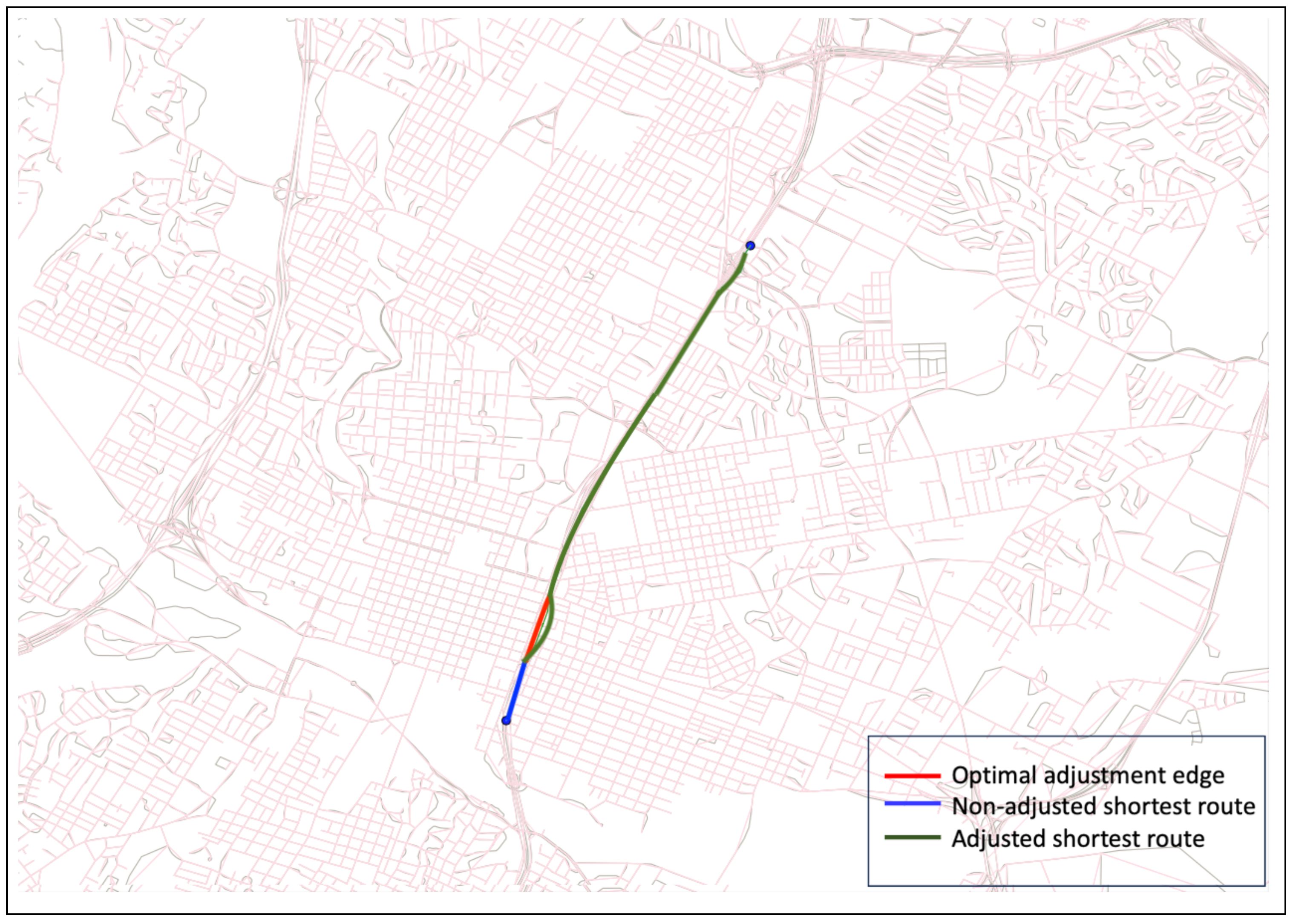
For the same source–destination pair,
and
, Theorem 1 prunes the original network to 50,628 edges and Theorem 2 yields a set of 2091 feasible adjustment edges. The routing algorithm(s) is (are) summarized in Algorithm 3 and the solutions are presented in
Figure 14. In the final steps of Algorithm 3, we use the popular Dijkstra’s shortest path algorithm to compute the shortest paths for original and adjusted routes.
| Algorithm 3 Non-Aggressive Adaptive Routing—Recursive Algorithm |
- Require:
The following are input parameters: - 1.
A road network with edge weights , depicting free flow times , low traffic probability and travel time due to high traffic ; - 2.
Source s, destination t, and maximum number of adjustment edges k; and - 3.
Routing model type , where - Ensure:
Optimal routing policy that minimizes expected travel time - 1:
function : - 2:
Create an empty set - 3:
for every do - 4:
Compute ,using Algorithm 1 - 5:
Compute set , using Algorithm 2 - 6:
Find an optimal edge that minimizes the expected travel time : (a) If model is Series Unforced Model, use ( 4) to compute (b) If model is Series Forced Model, use ( 6) to compute (c) If model is Parallel Model, use ( 8) to compute - 7:
if then - 8:
Append the optimal adjustment edge to - 9:
else Terminate - 10:
end if - 11:
end for - 12:
Derive that combines the shortest paths from source s to start node of every adjustment edge and finally to the destination t. Here, edge is adjustment edge with weight . Remaining edges assume expected times as their edge weights. - 13:
Derive for every adjustment edge, that combines the shortest paths from source s to destination t via the adjustment edge following the design presented in Section 3. Here, adjustment edge with weight . Remaining edges assume expected times as their edge weights. - 14:
return Optimal policy
|
4.3. Performance Evaluation
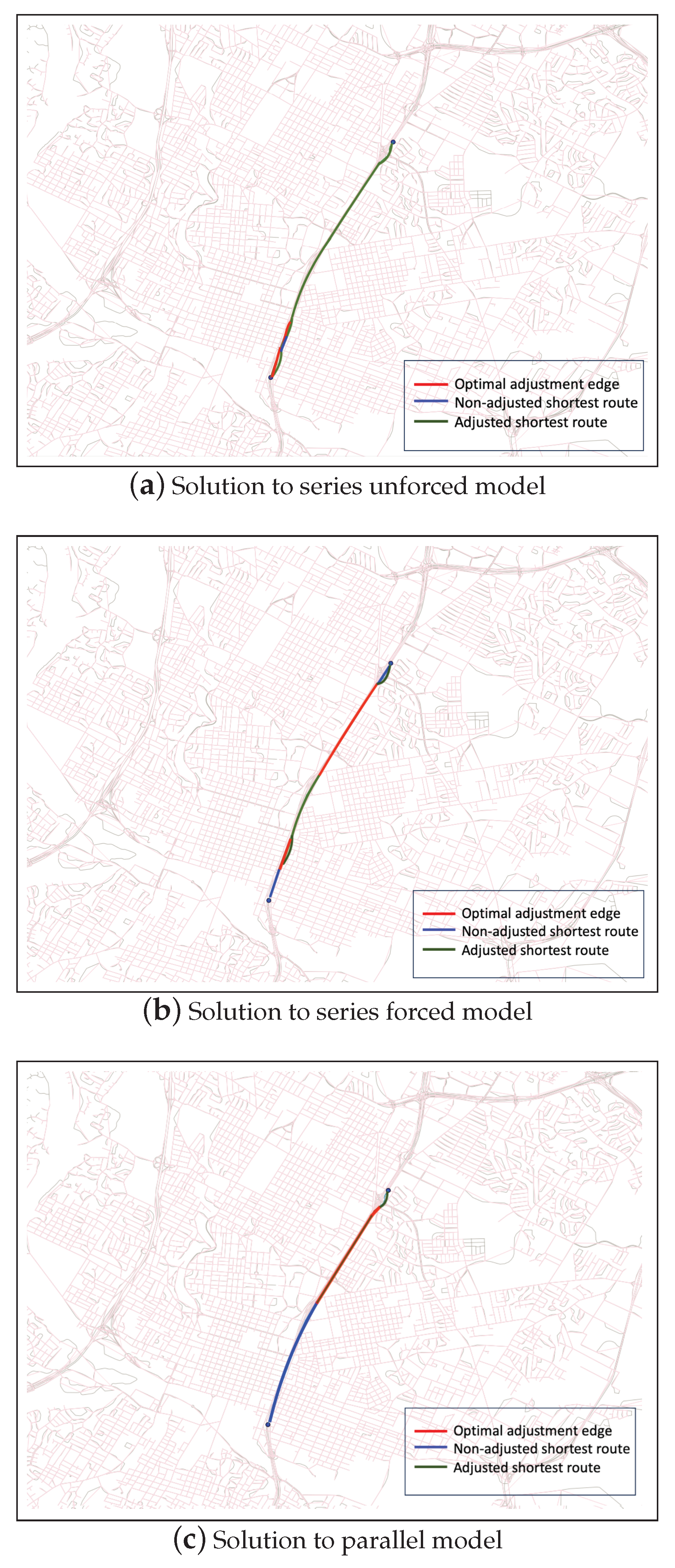
We conducted several computational experiments by implementing our algorithms in Python and solving it using MacOS 2.6 GHz Intel i5 processor with 8 GB RAM. We summarize the performance of our algorithms with respect to two adjustment edges, using the same example network as in
Figure 12, the parallel model performs the best in terms of reducing expected travel time. We save about 7% of travel time when compared to the single-route adjustment policy and about 13% compared to the fixed (non-adaptive) shortest path. Followed by parallel model, the series forced model performs better yielding about 3% savings compared to single-route policy and 9.5% savings compared to fixed path. Finally, the series unforced model provides the least savings, of less than
and 7%, respectively.
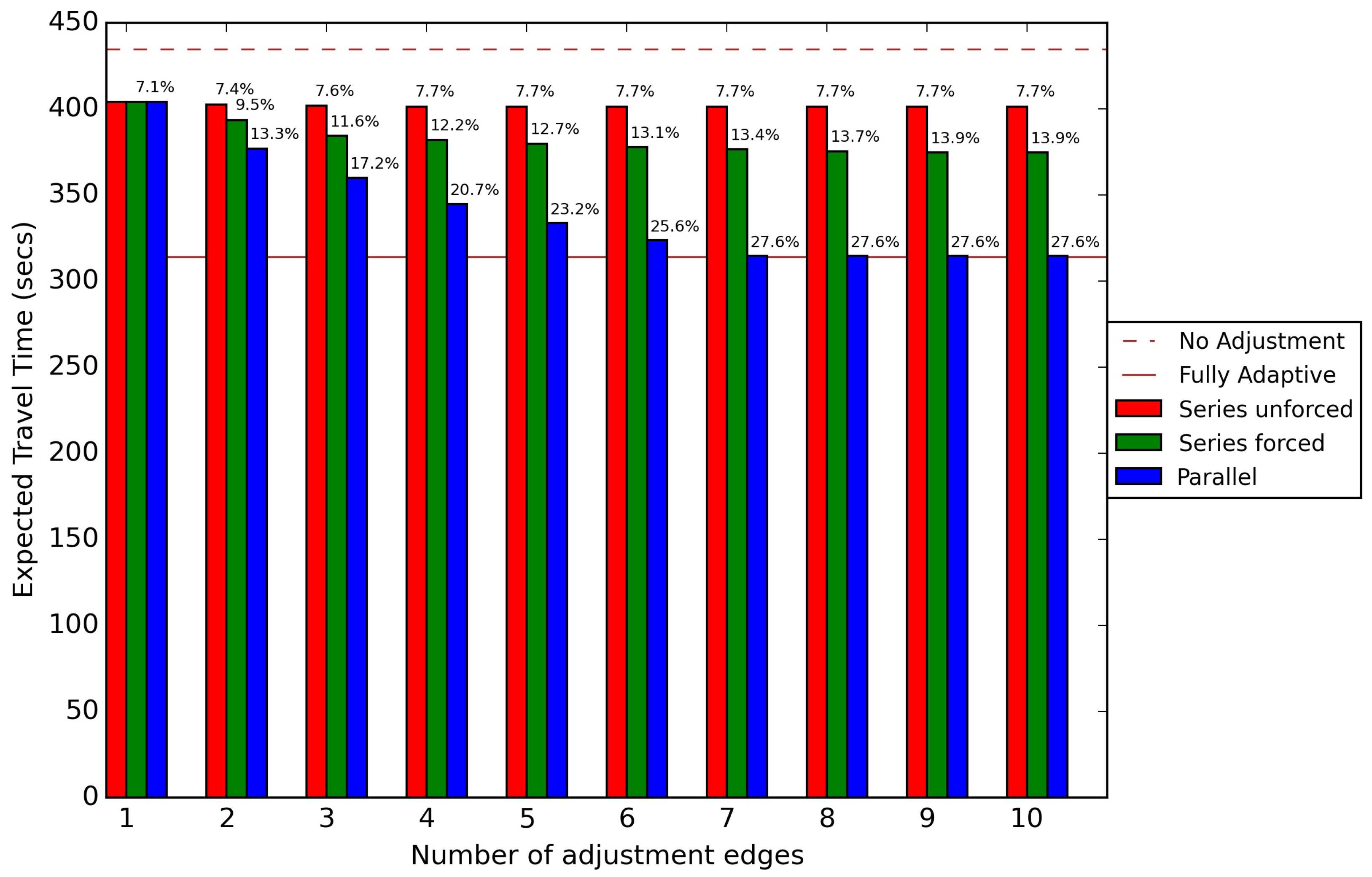
One can achieve more savings by increasing the number of route adjustments, albeit with a large increase in the computational effort. For the above example, the pruned network size for two adjustment edges is about 50% of the original network size and that of the three edges is almost the same as the original network, increasing the computational effort drastically. Thus, a trade-off arises between the number of edges to be observed for traffic and potential savings in expected travel times. In order to understand this trade-off, we solved our dynamic programming algorithms for different route adjustment models, on a smaller network consisting of 17,328 edges (given by the pruned network of the single-route adjustment model). The graph summarizing the benefit of adaptability is presented in
Figure 15.
It can be inferred from the graph that there is not much improvement in the expected travel time beyond two adjustment edges using the series unforced model. However, the series forced model yields about 2% reduction in expected travel time with three adjustment edges, after which the reduction deteriorates and tends to saturate. Similarly, the parallel model results in 3–5% reduction in the travel time up to seven adjustment edges, after which the reduction saturates. Thus, we can conclude that observing more than seven edges in this network instance, as opposed to CTP where all edges are decision points, does not contribute significantly to the reduction in travel time. We emphasize the fact that this summary is specific to the problem instance considered and the performance graph is likely to vary for different instances. Thus, choosing the right adjustment strategy and the right number of adjustments is a decision to be made by the user, based on the trade-off between the computational effort required and the anticipated reduction in expected travel times.
5. Conclusions
In this paper, we present a new way to route traffic in large networks. Our approach is called non-aggressive adaptive routing, and it allows the driver to make limited adjustments to routes while still minimizing the expected travel times. We propose three different routing strategies: series unforced, series forced, and parallel models. In every strategy, the driver observes the optimal adjustment edges for traffic and makes route adjustments in case of high traffic on the observing edge(s). However, where and how these adjustments are performed is the key differentiating factor to choose the right strategy.
We develop exact mathematical models to generate an optimal routing policy from each proposed strategy. In spite of our proposed dynamic programming algorithms being polynomially solvable, the algorithms may get intractable for medium to large sized networks. To alleviate this problem, we design some efficient bounds and present several theorems, to reduce the network size and compute a reduced feasible set of adjustment edges, leading to tractable algorithms.
Finally, we numerically assess the performance of our tractable algorithms using single- and two-route adjustment policies, and present the benefit of adaptability graph for an example source-destination pair in the Austin road network.
In terms of future extensions of this work, there is still scope to improve the tractability of our algorithms by developing even tighter lower bounds. There is also scope to studying other multiple route adjustment strategies; for example, one can consider a model where the driver is constrained to switching back and forth between two or more pre-computed routes. One can extend this model to account for correlation in traffic states between different edges. Another area of exploration will be using real-time traffic data from suitable sources, like unmanned aerial vehicles. Detecting tassels with imagery can provide instantaneous traffic information, in fact, factoring in the traffic information for different times of day might yield better results. Another possible future extension is to consider microscopic traffic factors like an individual vehicle’s position and velocity to further optimize the routing policies. We strongly believe that these extensions require significant additional research and therefore we defer their investigation to future work.


