Evaluation and Analysis of Heuristic Intelligent Optimization Algorithms for PSO, WDO, GWO and OOBO

Abstract

In order to comprehensively evaluate and analyze the effectiveness of various heuristic intelligent optimization algorithms, this research employed particle swarm optimization, wind driven optimization, grey wolf optimization, and one-to-one-based optimizer as the basis. It applied 22 benchmark test functions to conduct a comparison and analysis of performance for these algorithms, considering descriptive statistics such as convergence speed, accuracy, and stability. Additionally, time and space complexity calculations were employed, alongside the nonparametric Friedman test, to further assess the algorithms. Furthermore, an investigation into the impact of control parameters on the algorithms’ output was conducted to compare and analyze the test results under different algorithms. The experimental findings demonstrate the efficacy of the aforementioned approaches in comprehensively analyzing and comparing the performance on different types of intelligent optimization algorithms. These results illustrate that algorithm performance can vary across different test functions. The one-to-one-based optimizer algorithm exhibited superior accuracy, stability, and relatively lower complexity.

1. Introduction

In the realm of natural phenomena, diverse biological populations undergo evolutionary processes, resulting in the emergence of distinct sets of operational principles and behavioral patterns. To tackle complex optimization problems arising in practical applications, heuristic intelligent optimization algorithms are harnessed. These algorithms derive inspiration from the collective behavior observed in multi-biological populations encompassing avian, lupine, and botanical entities. By emulating information exchange mechanisms observed during group foraging, the heuristic intelligent optimization algorithm facilitates information interaction among individuals.

The inception of the heuristic intelligent optimization algorithm can be traced back to 1989, marked by the pioneering proposal of the ‘swarm intelligence’ concept by Gerardo Beni and Jing Wang [1]. By studying a large ensemble of uncomplicated individuals, researchers avoid the need for an intricate and elaborate internal design of the group system. Relying on simple rules, this method exhibits enhanced adaptability, stability, and robustness. The heuristic intelligent algorithm possesses the following distinctive characteristics: accelerated optimization speed and the ability to effectively explore global optimal solutions for complex optimization problems. The individuals constituting the studied population are spatially distributed, devoid of central control, and extensible. The distribution of individuals is straightforward, allowing for convenient functional realization [2]. Particle swarm optimization (PSO) [3,4,5], wind driven optimization (WDO) [6,7], and grey wolf optimizer (GWO) [8,9] constitute a subset of commonly employed heuristic intelligent optimization algorithms. These algorithms offer researchers the means to tackle a wide range of problems including the determination of the optimal function values (e.g., the traveling salesman problem), objective assignment, and job scheduling, among others. The heuristic intelligent optimization algorithm represents a particular type of optimization method that often encounters challenges when seeking a precise or even feasible solution in complex real-world scenarios. As a result, it is applied to approximate the optimal solution and serve as a representation of the final results.

As time passes, a variety of heuristic intelligent optimization algorithms have emerged. However, the accurate evaluation of optimization performance and the determination of suitable circumstances for using corresponding intelligent optimization algorithms remain significant challenges in the development of these algorithms. Currently, the widely adopted approach for evaluating heuristic intelligent optimization algorithms involves utilizing different types of test functions, running the algorithms independently, and then calculating statistical parameters such as the average value, standard deviation, best value, and worst value for comparison and evaluation. However, this analysis method tends to provide one-sided results and lacks a unified qualitative analysis, especially when dealing with multiple unimodal and multimodal test functions. Due to the abundance of test data results, accurately evaluating and comparing the performance of heuristic intelligent optimization algorithms becomes more difficult, rendering this method of limited significance in guiding practical applications [10].

Therefore, this study aimed to compare and evaluate the performance of four heuristic intelligent optimization algorithms, namely particle swarm optimization (PSO), wind driven optimization algorithm (WDO), grey wolf optimizer (GWO), and one-to-one-based optimizer (OOBO), from four perspectives. These perspectives include conducting descriptive statistical analysis of the algorithms in terms of stability and convergence, discussing the algorithms’ complexity in terms of space and time, and employing the Friedman test in nonparametric statistics to assess whether there are significant differences be-tween the algorithms. Simultaneously, this paper also analyzed the influence of the algorithm control parameters on the optimization results. Finally, through comprehensive comparison, the strengths and weaknesses of the four algorithms are summarized.

2. Algorithm Description

This paper conducted an analysis of three prominent intelligent optimization algorithms: particle swarm optimization (PSO), wind driven optimization (WDO), and grey wolf optimization (GWO) algorithms.

2.1. Particle Swarm Optimization

The particle swarm optimization (PSO) algorithm was developed by American academics to emulate the foraging behavior observed in birds and other animals [11,12,13]. In the wild, birds often demonstrate both interpersonal and group cooperation during foraging. While some birds forage alone, others engage in collective foraging. During this process, certain dominant birds possess valuable information and guide the others to food sources.

In the particle swarm optimization technique, each solution within the target space is represented by a bird or particle. The goal of the flock is to find the desired food source, which corresponds to the optimal solution for the problem at hand. Each particle exhibits individual and collective behaviors while seeking the best answer. To determine the optimal solution, each particle learns from the experiences of both its peers and itself. It adapts its velocity and position based on its own history and the overall best value attained by the entire swarm. The quality of each position is evaluated using a fitness value, which aligns with the objective function of the optimization problem [14,15].

The particle swarm optimization technique adheres to the following three guidelines for ongoing optimization and adjustment [16]:

• Particles maintain a safe distance from the nearest individual to prevent collisions between particles.
• Each particle aims to approach the target value as closely as possible.
• The particles strive to converge toward the center of the target population.

2.1.1. Parameter Setting for Particle Swarm Optimization Algorithm

A particle swarm in an E-dimensional target search space consists of M particles. Each particle is represented by an E-dimensional vector, and its position x_i in space can be described by Formula (1) [17].

$$x_i=\{x_{i1},x_{i2},\cdots ,x_{iE}\},i=1,2,\cdots ,M$$

(1)

The spatial position of a particle represents a solution to the target optimization problem. This position can be evaluated by inputting it into the fitness function, resulting in a fitness value that indicates the quality of the particle. Additionally, the flying speed K_i of a particle is represented by an E-dimensional vector, which can be obtained from the target optimization problem solution and calculated using Formula (2).

$$K_i=\{K_{i1},K_{i2},\cdots ,K_{iE}\},i=1,2,\cdots ,M$$

(2)

Within a specified border range, the position and speed of the particle are created at random.

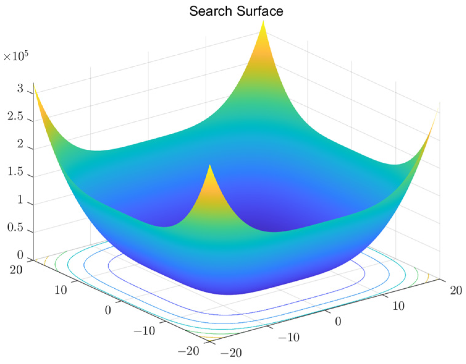
2.1.2. Physical Model Building and Particle Swarm Updating Method

Formula (3) can be utilized to express the individual i particle’s historical best position P_best, which indicates the position it has traversed through with the best fitness value.

$$p_{best}=\{p_{besti1},p_{besti2},\cdots ,p_{bestiE}\},i=1,2,\cdots ,M$$

(3)

Formula (4) can be employed to denote the global historical best position q_best, which represents the best location that the entire particle swarm has traversed through.

$$q_{best}=\{q_{besti1},q_{besti2},\cdots ,q_{bestiE}\},i=1,2,\cdots ,M$$

(4)

Position update and velocity update are two fundamental operations employed in particle swarm optimization. The velocity update can be described using Formula (5) [18].

$$K_{ij}(t+1)=w{K}_{ij}(t)+c_1{r}_1(p_{bestij}(t)-x_{ij}(t))+c_2{r}_2(q_{bestj}-x_{ij}(t))$$

(5)

Formula (6) can be utilized to describe the process by which a particle swarm updates its positions.

$$x_{ij}(t+1)=x_{ij}(t)+K_{ij}(t+1)$$

(6)

In Formula (5), the subscript i represents the i particle, while the subscript j represents the j dimension of the particle’s position. The value t corresponds to the current iteration count. The acceleration constant parameters c₁ and c₂ typically fall within the range of 0 and 2. The values of the mutually independent parameters r₁ and r₂, which range between 0 and 1, are randomly generated. As can be deduced from the representation of Formula (5), particles adeptly acquire knowledge from their individual exploration as well as their collective search encounters to gradually approach the most optimal solution. The synergetic effect of parameters c₁ and c₂ facilitates the amalgamation of insights gained through individual learning and group dynamics. w is the inertia coefficient, which takes the value of 1 for the particle swarm optimization algorithm in this paper.

2.1.3. Algorithm for Particle Swarm Optimization: Fitness Function Selection

The evaluation of individuals (or solutions) is carried out based on their objective function values throughout the entirety of the particle swarm optimization search process. An iterative scheme is then employed to adapt the positions and velocities of the particle swarm, leveraging these values as guiding principles for updates. This systematic integration of objective function values ensures the continuous enhancement of initial solutions toward the attainment of the global optimum.

2.1.4. Identify the Particle Swarm Optimization Algorithm’s Border Range

In order to maintain the integrity of particle placements and speeds within the particle swarm optimization, boundaries are defined. Consequently, particle units are restricted to the upper boundary value when surpassing the upper limit, and limited to the lower boundary value when falling below the lower limit. This adherence to boundary conditions is expressed by Equation (7), which serves to capture constraints imposed on particle swarm units.

$$u_{new}=\left\{\begin{array}{l}ub,u>u_{\max }\\ Ib,u<u_{\min }\end{array}\right.$$

(7)

where ub and Ib in Equation (7) stand for the variable’s upper and lower bounds, respectively.

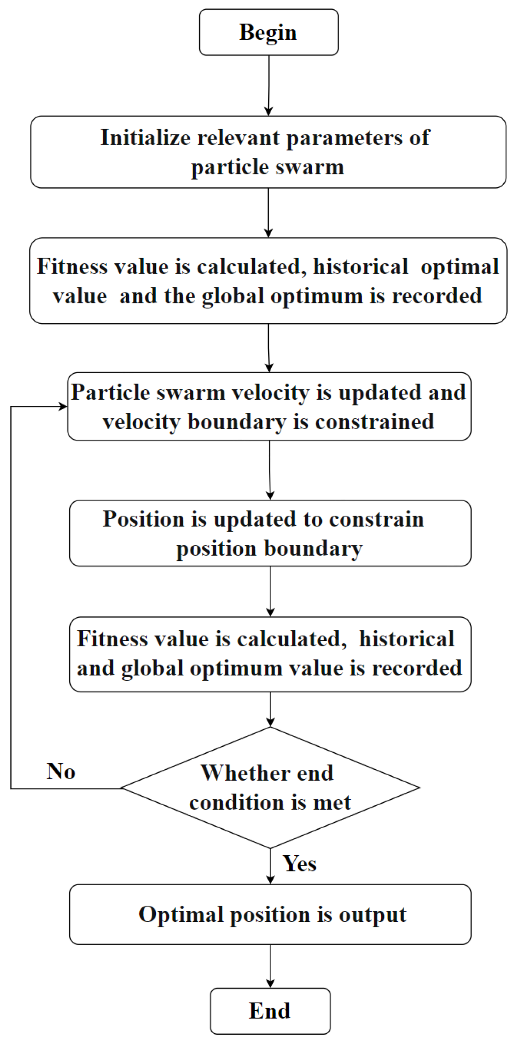
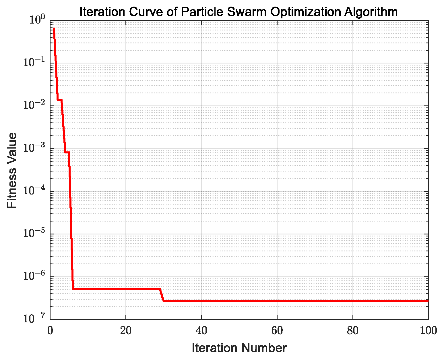
2.1.5. The Particle Swarm Optimization Algorithm’s Process

Figure 1 illustrates the flowchart of the particle swarm optimization algorithm, providing a detailed outline of the precise computational steps involved. Here is a refined expression of the algorithm:

Step 1: Set the necessary parameters for the particle swarm, which include the maximum number of iterations, position boundary range, and velocity boundary range.

Step 2: Calculate the fitness value of each particle based on the given fitness function and record both the historical best value and the global best value encountered.

Step 3: Update the particle velocities, restricting them within the defined bounds to prevent exceeding barriers.

Step 4: Update the positions of the particles, constraining them within the specified boundary limits.

Step 5: Recalculate the fitness value for each particle using the fitness function.

Step 6: For each individual particle, compare its fitness value to its previous best value. If the new value is greater, update the historical best value accordingly.

Step 7: For each particle, compare its fitness value to the best value encountered by the entire swarm. If the current value is higher, update the global best value accordingly.

Step 8: Check if the termination condition has been met. If the maximum number of iterations has been reached, output the optimal position. If not, repeat Steps 3–8 for further iterations.

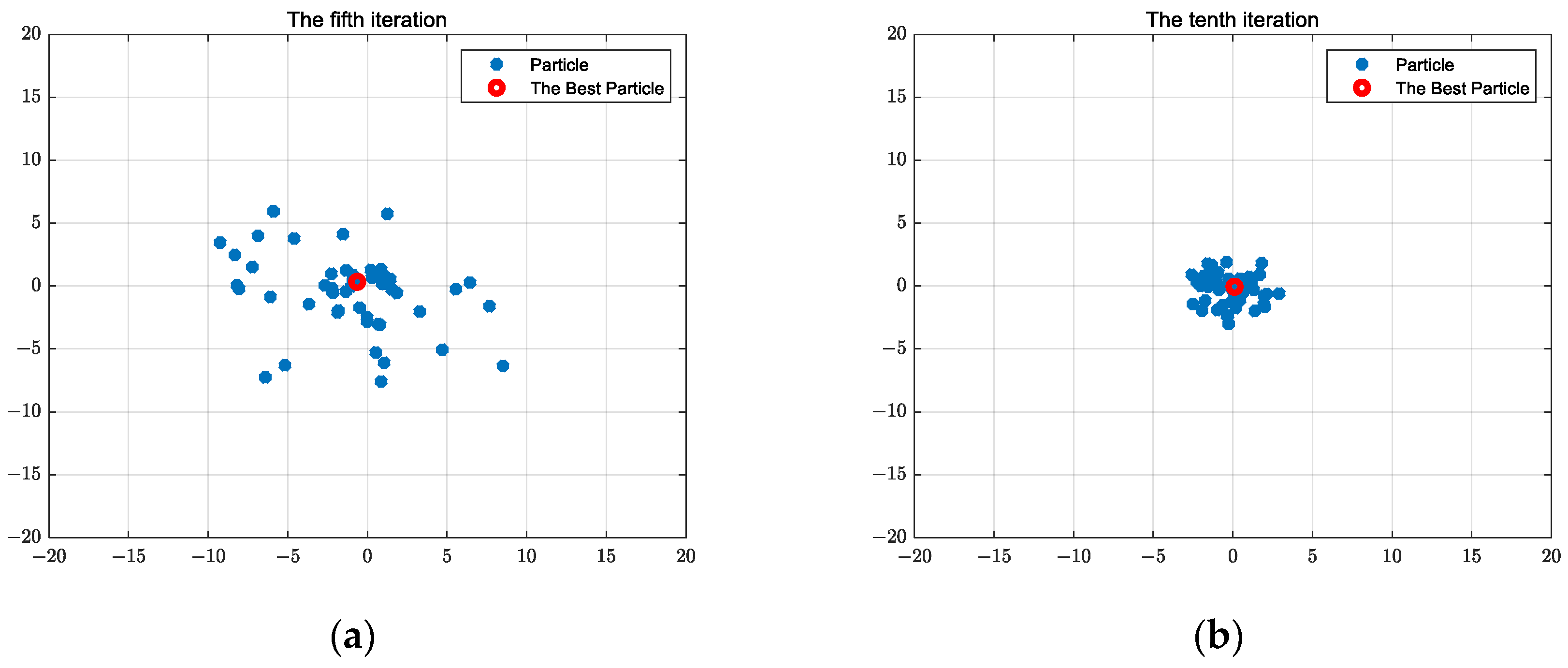
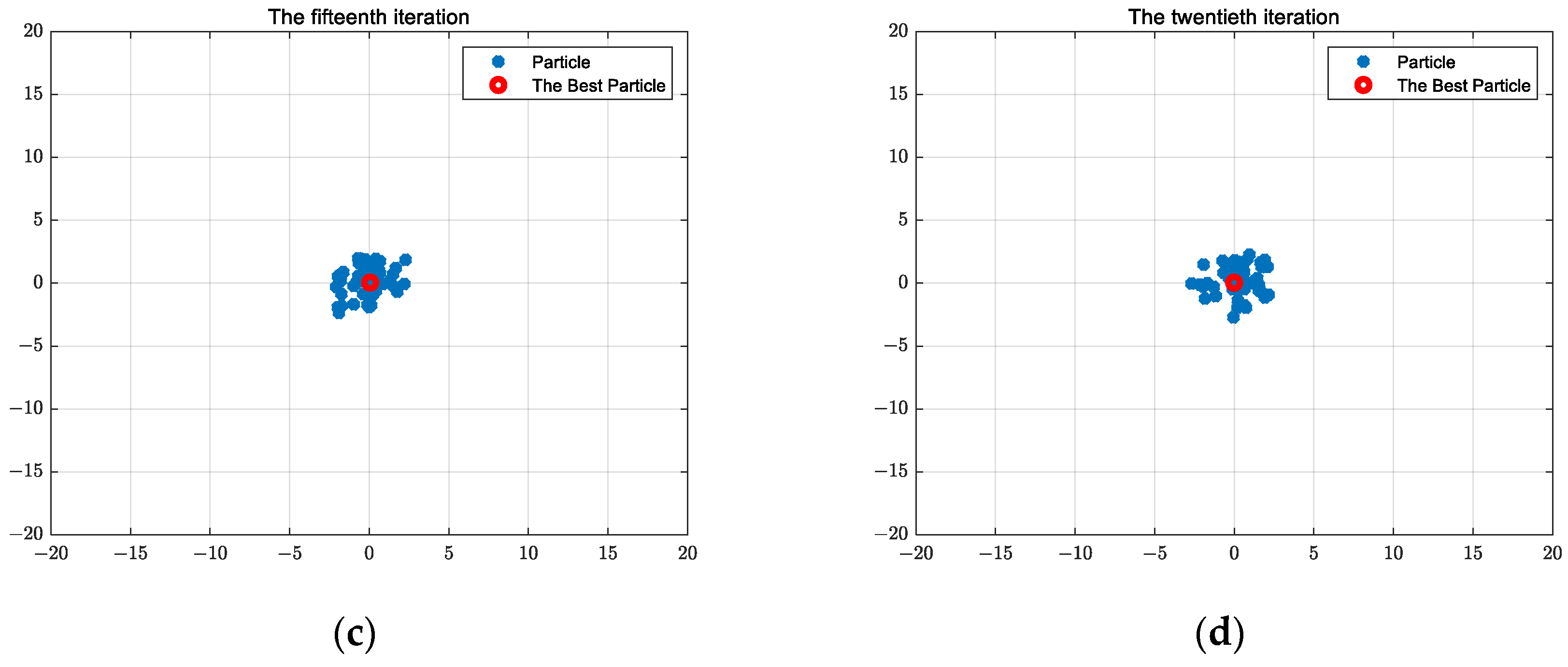
2.1.6. Particle Swarm Optimization Algorithm Calculation Results

By incorporating the aforementioned computational steps, we can leverage the particle swarm optimization approach to tackle the following problem: Determine the values of x₁ and x₂ that minimize the function represented by Equation (8).

$$f(x_1,x_2)=x_1{}^4+x_2{}^4$$

(8)

In Equation (8), the variables x₁ and x₂ are confined within the range of [–20, 20]. Figure 2 visually depicts the search space of the function represented by Formula (8).

According to Figure 2, intently scrutinizing the function expression and the corresponding search space, it becomes evident that the function’s minimum value is 0. This finding implies that the optimal solution for this problem is achieved when variables x₁ and x₂ attain values of 0 each. To facilitate the particle swarm optimization technique’s implementation in tackling this problem, certain parameters were set. These include a population size of 50 and a maximum number of iterations capped at 100. Given that x₁ and x₂ are the variables being solved, the particle dimension was fixed at 2. Furthermore, the upper and lower limits for the particles were established as ub = [20, 20] and lb = [−20, −20], respectively. The velocity of the particles was also controlled within specific bounds, with the upper and lower limits being set as K_max = [2, 2] and K_min = [−2, −2], respectively.

Figure 2 represents the fitness function designed to align with the optimization objective at hand. On the other hand, Figure 3 depicts the iteration curve of the program, showcasing the progression of the particle swarm optimization technique over time. After running the optimization algorithm, the obtained results indicate that x₁ was approximately equal to −0.010188, and x₂ was approximately equal to −0.0028668. The function value corresponding to this ideal solution was calculated to be 1.0841 × 10⁻⁸, suggesting a highly accurate approximation. The final position coordinates (−0.010188, −0.0028668) derived through the particle swarm optimization algorithm closely approached the theoretically ideal values of (0, 0), demonstrating the effectiveness of the algorithm in yielding close-to-optimal solutions.

Figure 4 offers intermediate results that aid in understanding the dispersion of particles within each generation during the optimization process. It provides insightful visuals of the particle positions in each generation including the position of the best particle at each step. Additionally, Figure 4 highlights that the whole particle swarm gradually converged toward the optimal position of (0, 0). This clearly demonstrates the persistent movement of the particle swarm toward the globally optimal solution.

2.2. Wind Driven Optimization Algorithm

The wind driven optimization method, proposed by Bayraktar Z and others in 2010 [19,20], is an intelligent optimization algorithm that incorporates Newton’s Second Law of motion force acceleration and the ideal gas equation. By simulating the motion of air particles under the influence of forces, this method constructs a simplified model representing the movement of particles in the air. These equations govern the updates of velocity and the position of air particles throughout each iteration cycle. As a technique inspired by the study of forces and the motion of air particles in the atmosphere, wind driven optimization exhibits a strong physical basis. It possesses the ability to strike a balance between global exploration and local exploitation, effectively enhancing its optimization capabilities.

2.2.1. Parameterization of the Wind Driven Optimization Algorithm

Given the assumption that the dimension of each air particle in the population X pop is denoted as E, the population can be represented by a matrix of dimensions pop × E. This matrix, as described by Formula (9), encapsulates the configuration of the population, where each row corresponds to an individual particle and its E-dimensional position.

$$X=\left(\begin{array}{ccc}{x}_1^1& \dots & x_1^E\\ ⋮& \ddots & ⋮\\ x_{pop}^1& \cdots & x_{pop}^E\end{array}\right)$$

(9)

Considering the influence of location on air particles, the selection of parameter values should be based on the specific context of the real-world application. It is customary to determine the range of values for each parameter that reflects the problem’s characteristics. In Section 2.2.4, a precise set of ranges is delineated for the parameters, enabling the generation of the initial air particles. The values for these particles were randomly selected from their respective ranges, facilitating the exploration of diverse regions within the search space.

2.2.2. Method for Establishing Physical Models and Updating Air Units

The wind driven optimization technique is a mathematical algorithm that aims to replicate the movement of the atmosphere caused by changes in the local air pressure. Eventually, a state of equilibrium is reached through this process. This algorithm models the motion of an abstract air particle unit, taking into account four forces: gravity, Coriolis force (resulting from the rotation of the Earth), the air pressure gradient force (directed from high pressure to low pressure), and the frictional force acting on the air pressure gradient force. By incorporating Newton’s Second Law and the ideal gas equation, these four forces are combined into a set of equations. Through this process, a position updating formula for the wind driven optimization method can be derived [21]. The detailed procedure is outlined as follows.

Varied air densities and pressures will occur from varied regional temperatures. Air will go from a high-pressure area to a low-pressure area due to differences in atmospheric pressure. Pressure gradient, which may be determined by changes in distance, is what causes gas flow. In the Cartesian coordinate system, this is denoted by Formula (10).

$$\Delta P=\left(\frac{\delta P}{\delta x},\frac{\delta P}{\delta y},\frac{\delta P}{\delta z}\right)$$

(10)

Equation (11) is modified by adding a negative sign to represent the direction of decreasing pressure gradient when air moves from a high-pressure to a low-pressure region. Equation (11) can be used to depict the pressure gradient F_PG while taking into account the restricted mass and air volume.

To incorporate the directionality of air moving from a high-pressure region to a low-pressure region, Equation (11) is modified by adding a negative sign. This modification reflects the decreasing nature of the pressure gradient in such cases. Equation (11) can be utilized to represent the pressure gradient, denoted as F_PG, while considering the restricted mass and air volume.

$$F_{PG}=-\Delta P\delta V$$

(11)

In an abstract wind model, we make the assumption that the atmosphere is uniform and the fluids are in hydrostatic equilibrium. In a Cartesian coordinate system, the fluid dynamics equation states that the horizontal airflow is more prominent than the vertical airflow. This implies that we consider the wind to predominantly move in the horizontal direction, and changes in horizontal pressure are the primary driver of wind movement. According to Newton’s Second Law of Motion, the magnitude of the acceleration vector, denoted as a, operating in the direction of the net force on an air unit, can be expressed as follows.

$$\rho a={\displaystyle \sum F_i}$$

(12)

In this context, we can employ an equation that establishes the relationship between air pressure, density, and temperature, allowing us to apply the gas laws. The density of a small air unit can be denoted as ρ, while the force acting on it is represented by F_i. By utilizing the following gas laws, we can determine the interconnections among air pressure, density, and temperature.

$$P=\rho RT$$

(13)

In Equation (13), let P represent pressure, R denote the universal gas constant, and T symbolize temperature.

Equation (14) simplifies the friction force acting on the atmosphere, which serves as the resistance to the movement of an air parcel, despite the pressure gradient force being the fundamental force that initiates the movement.

Equation (14) succinctly represents the complex friction force acting on the atmosphere, which opposes the movement of an air parcel. It is important to note that the primary force responsible for the motion of an air parcel is the pressure gradient force.

$$F_F=-\rho au$$

(14)

In Equation (14), let a symbolize the vector velocity of the wind, and u represent the friction coefficient.

Gravity, denoted as F_G, is a force that acts perpendicular to the Earth’s surface in three-dimensional space. However, to simplify its representation, we can assume the origin of the rectangular coordinate system to be located at the center of the Earth.

$$F_G=\rho \delta Vg$$

(15)

The rotation of the Earth induces rotation of the reference coordinate system, leading to an amplification of Coriolis force. The Coriolis force results in the deflection of wind direction from its original path, with the deflection angle being directly influenced by the Earth’s rotation. This phenomenon is also influenced by the latitude of the atmosphere and the velocity of the air unit. The definition of the Coriolis force is as follows.

$$F_G=-2\mathrm{\Omega }\times u$$

(16)

In Equation (16), let Ω symbolize the rotation of the Earth.

By considering various forces acting on the air parcel including the Coriolis force, gravitational force, frictional force, and pressure gradient, we can substitute Equations (11), (14)–(16) into the right-hand side of Equation (12) to obtain the expression.

$$\rho \frac{\Delta u}{\Delta t}=(\rho \delta Vg)+(-\Delta P\delta V)+(-\rho au)+(-2\mathrm{\Omega }u)$$

(17)

Equation (9) can be simplified to Equation (18) by introducing the assumption of a temporal difference.

$$\rho \Delta u=\rho g+(-\Delta P)+(-\rho au)+(-2\mathrm{\Omega }u)$$

(18)

Utilizing Equation (6), the relationship between density ρ and pressure can be established. This allows us to express density in terms of pressure. Furthermore, in Equation (19), the substitution of temperature and the universal gas constant is made.

$$\frac{P_{cur}}{RT}\Delta u=(\frac{P_{cur}}{RT}g)-\Delta P-\frac{P_{cur}}{RT}au+(-2\mathrm{\Omega }u)$$

(19)

The variable P_cur represents current pressure in this context. Equation (20) is derived by dividing both sides of Equation (11) by the term P_cur/RT.

$$\Delta u=g-\Delta P\frac{P_{cur}}{RT}-au+(-2\mathrm{\Omega }uRT/P_{cur})$$

(20)

The parameter u_cur represents the current velocity value, indicating the velocity for the present iteration. Equation (21) is obtained by substituting the value of variable w into Equation (12).

$$u_{new}=(1-a)u_{cur}+g+(-\Delta P\times RT/P_{cur})+(-2\mathrm{\Omega }\times uRT/P_{cur})$$

(21)

The vector representing the force of gravity, denoted as g, is given by g = |g|(0 − x_cur). A pressure gradient, denoted as P, can be defined as the force that propels an air unit toward its ideal pressure point. Hence, the magnitude of P is equal to the difference between the air unit’s current pressure, P_cur, and its ideal pressure, P_opt. The direction of the pressure gradient points from the current position x_cur to the ideal position x_opt. Equations (22) and (23) offer a clear and concise representation of this concept.

$$\Delta P=\left|P_{new}-P_{opt}\right|(x_{cur}-x_{opt})$$

(22)

$$u_{new}=(1-a)u_{cur}+g{x}_{cur}-\left|P_{new}-P_{opt}\right|(x_{cur}-x_{opt})\times RT/P_{cur}-2\mathrm{\Omega }\times uRT/P_{cur}$$

(23)

The Coriolis force, as defined in Formula (23), is given by the vector product of the Earth’s rotational speed and the unit air acceleration. To illustrate the influence of the Coriolis force, we can consider replacing it with another air unit that possesses the same velocity $u_{cur}^{other\dim }$. By substituting the simplified Coriolis force into Formula (23), the resulting Formula (24) yields relevant outcomes.

$$u_{new}=(1-a)u_{cur}+g{x}_{cur}-\left|P_{new}-P_{opt}\right|(x_{cur}-x_{opt})\times RT/P_{cur}+(\frac{c\times u_{cur}^{other\dim }}{i})$$

(24)

The efficiency of the wind driven optimization algorithm can potentially be affected when there is an increase in wind speed to avoid excessively high pressure values. To address this, all air units can be organized in descending order based on their pressure values [22]. This arrangement allows us to express Equation (16) as Equation (25), presented below.

$$u_{new}=(1-a)u_{cur}+g{x}_{cur}+(x_{cur}-x_{opt})\times RT\left|1/i-1\right|+(\frac{c\times u_{cur}^{other\dim }}{i})$$

(25)

In Equation (25), the variable i represents the ranking of each individual air unit. From this, we can derive the subsequent equation for updating the positions of the air units.

$$x_{new}=x_{cur}+(u_{new}\Delta t)$$

(26)

In Formula (26), the variable x_cur represents the current position of the air unit in the search space. On the other hand, u_new represents the newly updated position of the cycle state. During each iteration, all air units within the search area move in random directions and speeds. The speed and position of each air unit, as given in Equations (17) and (18), are modified to ensure that it continuously approaches the ideal position.

2.2.3. Algorithm for the Wind Driven Optimization: Fitness Function Selection

In the wind driven optimization algorithm, the value of the pressure function, also referred to as the fitness function, plays a crucial role. It not only helps in evaluating the advantages and disadvantages of a candidate solution, but also forms the basis for updating the position of the air unit in subsequent iterations. As the algorithm progresses, the initial solution gradually moves closer to the optimal solution based on the information provided by the pressure fitness.

2.2.4. Identify the Wind Driven Optimization Algorithm’s Boundary Range

Air units should be able to move within a specific range for each dimension. When the position of the air unit is above the upper limit, only the upper boundary value is used. The boundary value is only used when the air unit is lower than the boundary below. As a result, Formula (27) illustrates the air unit position limits.

To ensure that the movement of the air units remains within a predetermined range for each dimension, certain constraints are implemented. If the position of an air unit exceeds the upper limit, the value is set to the upper boundary limit. Similarly, if the position falls below the lower boundary, only the lower boundary value is taken into account. This arrangement is illustrated by Formula (27), which captures the position limits imposed on the air units.

$$u_{new}=\left\{\begin{array}{l}ub,u>u_{\max }\\ Ib,u<u_{\min }\end{array}\right.$$

(27)

The upper and lower limits of the air unit dimension in Equation (27) are denoted by ub and Ib, respectively.

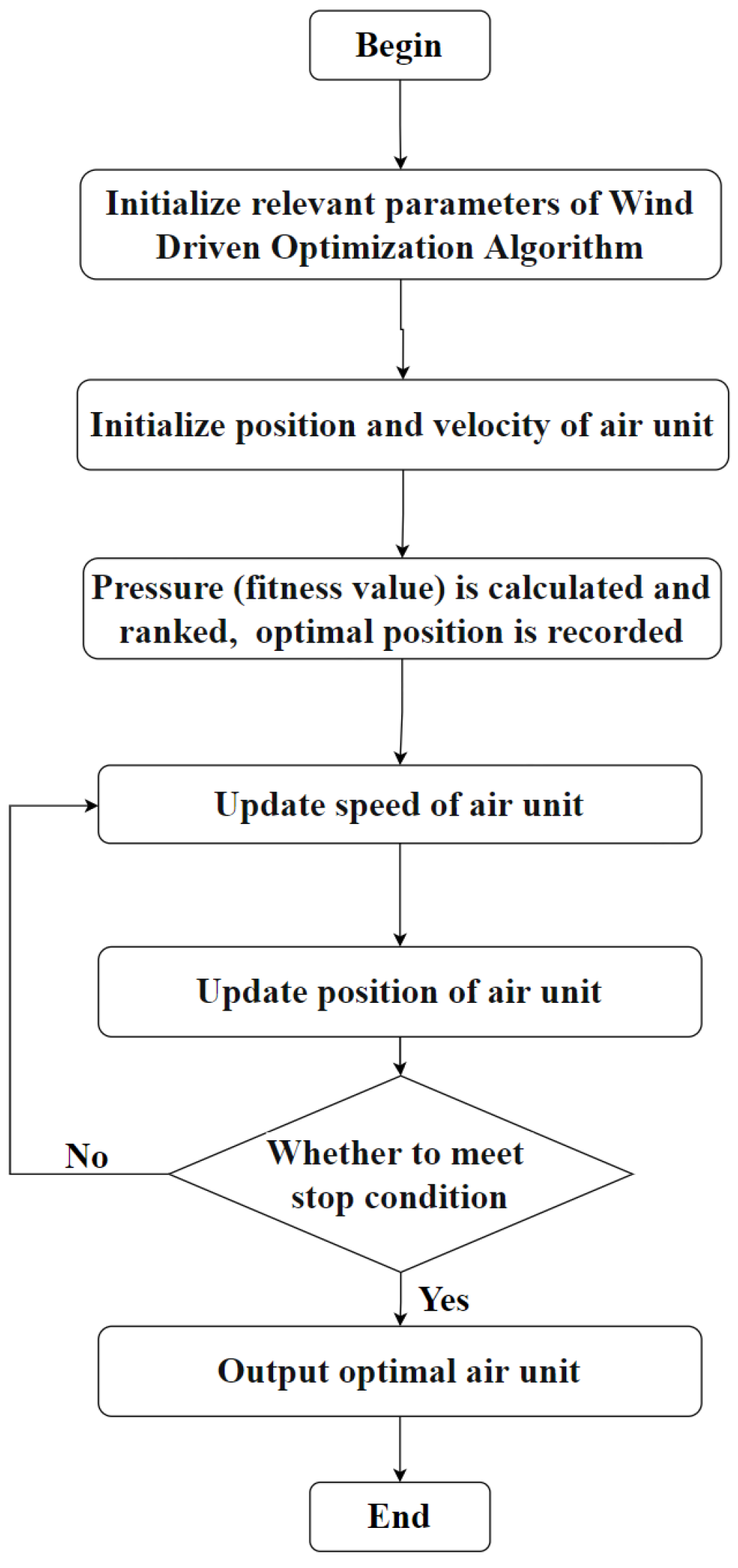
2.2.5. The Wind Driven Optimization Algorithm’s Process

Figure 5 represents the flowchart for the wind driven optimization algorithm. It outlines the precise calculation steps as follows.

Step 1: Initialize the population size, define the pressure function (fitness function), set the maximum number of iterations and relevant parameters, and establish the search boundaries.

Step 2: Set the initial position and speed of each air unit to zero.

Step 3: Calculate the position and velocity of each air unit for the current iteration.

Step 4: Update the speed of each air unit based on certain criteria.

Step 5: Adjust the positions of the air units according to their updated speed.

Step 6: Verify whether all constraint conditions are met. If yes, determine the best air unit. If not, repeat Steps 2 to 5 until the conditions are satisfied.

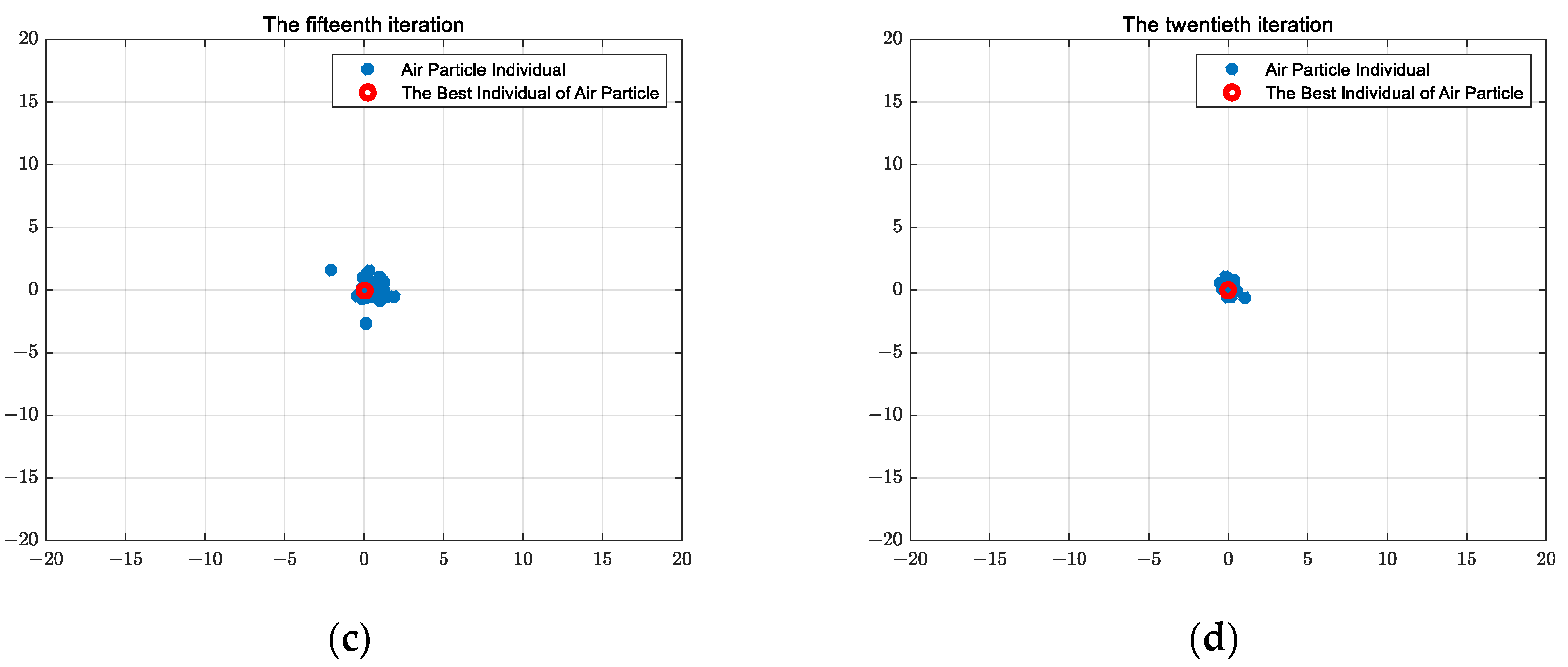
2.2.6. Wind Driven Optimization Algorithm Calculation Results

In addition to the computational framework described previously, the wind driven optimization algorithm was employed to tackle the given optimization problem, which involves minimizing the value of the following function (Formula (8)) with respect to a pair of variables, x₁ and x₂.

The value ranges of x₁ and x₂ in Formula (8) can be represented as [−20, 20]. To visualize the search space for the function in Formula (8), refer to Figure 2.

The minimal value of the Formula (8) function is 0, and the optimal solution is obtained when x₁ = 0 and x₂ = 0, as evident from both the function expression and the search space depicted in Figure 2. To address this problem, we can employ a technique called wind driven optimization. In this approach, the maximum number of iterations is set to 100, and the population size is 50. Each individual air unit is characterized by a dimension of 2, with an upper boundary of [20, 20] and a lower boundary of [−20, −20], as the values of x₁ and x₂ have already been determined. To facilitate the wind driven optimization, certain constants are employed such as the gravitational constant g = 0.2, RT = 3 and other relevant constants associated with this technique. The constant in the update formula is set to 0.4, and the Coriolis force is denoted as c = 0.4. Additionally, the lower and upper velocity boundaries are defined as 0.3 times the upper bound (ub) and lower bound (Ib), respectively.

The fitness function, Formula (8), was devised to align with the objective of the optimization problem. The program’s iteration curve is depicted in Figure 6. Ultimately, the optimal solution is achieved with a function value of 7.782 × 10⁻³⁴ and the corresponding values of x₁ = −1.0462 × 10⁻⁹ and x₂ = −5.2797 × 10⁻⁹, as obtained from the output of the wind driven optimization method. Notably, the final solution (−1.0462 × 10⁻⁹, −5.2797 × 10⁻⁹) determined by the wind driven optimization technique closely approximates the theoretical optimal value (0, 0). This indicates that the wind driven optimization algorithm exhibits strong optimization capabilities.

In order to gain a deeper insight into the distribution of air units within each generation during both the initial and subsequent iterations, it is beneficial to examine the changes in the positions of individuals within the air units. These variations are illustrated in Figure 7, along with the intermediate discoveries made by the algorithm. Additionally, the positions of the individuals in each generation’s air units can be observed simultaneously. Figure 7 effectively demonstrates that as the number of iterations increases, the individuals within the air units progressively converge toward the optimal location (0, 0). This observation indicates that the air units consistently move toward their ideal positions, showcasing the algorithm’s ability to converge toward the optimal solution.

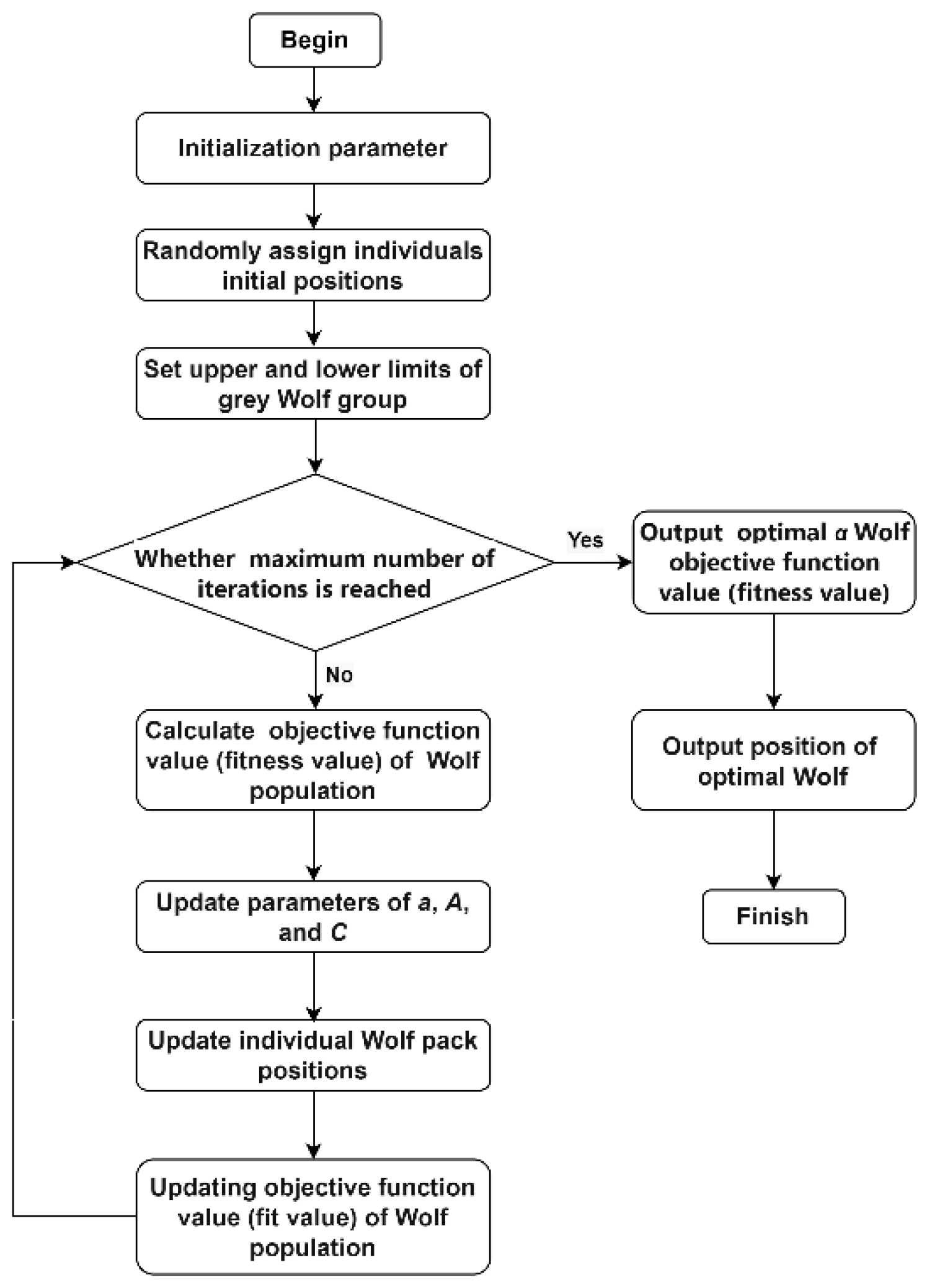
2.3. Grey Wolf Optimization Algorithm

The grey wolf optimizer algorithm (GWO) was introduced by Seyedali Mirjalili, an esteemed researcher from Australia [23,24]. Inspired by the natural patterns of predation observed in grey wolf groups, this algorithm utilizes a cooperative process among wolves to accomplish its optimization objectives. By simulating the behavior of wolves, the GWO algorithm leverages their hunting strategies and social dynamics to achieve efficient optimization.

The grey wolf optimizer method is built upon the hierarchical social structure observed in a grey wolf population, which consists of four levels shaped like pyramids. At the apex of the hierarchy is the highest-ranking α₁ wolf, followed by the α₂ wolf, α₃ wolf, and finally the lowest-ranking α₄ wolf. The α₁ wolf, being the leader of the pack, holds authority over the α₂ wolf, α₃ Wolf, and α₄ wolf. The α₂ wolf, as the second-in-command, is responsible for overseeing the α₃ wolf and α₄ wolf, while also providing assistance to the α₁ wolf. The α₃ wolf supports the α₁ wolf and α₂ wolf, and serves as the foundation of the wolf pack. The majority of the pack consists of α₄ wolves, who are subordinate to the α₁ wolf, α₂ wolf, and α₃ wolf [25].

2.3.1. Trapping Prey

Formulas (28)–(32) are integral components of the grey wolf optimizer algorithm, serving the purpose of iteratively updating the positions of the wolves.

$$\mathit{B}=\left|\mathit{C}\mathbf{•}{\mathit{Y}}_{\mathit{p}}\mathbf{\left(}\mathit{t}\mathbf{\right)}\mathbf{-}\mathit{Y}\mathbf{\left(}\mathit{t}\mathbf{\right)}\right|$$

(28)

$$\mathit{Y}\left(\mathit{t}\mathbf{+}\mathbf{1}\right){\mathbf{=}\mathit{Y}}_{\mathit{p}}\mathbf{\left(}\mathit{t}\mathbf{\right)}\mathbf{-}\mathit{A}\mathbf{•}\mathit{B}$$

(29)

$$\mathit{A}=2a\times {\mathit{r}}_1-a$$

(30)

$${\mathit{C}\mathbf{=}\mathbf{2}\mathit{r}}_{\mathbf{2}}$$

(31)

$$a=2-\frac{2t}{t_{max}}$$

(32)

In the grey wolf optimizer algorithm, the prey’s position vector is denoted as Y_p, and it is updated using Formulas (28) to (32). On the other hand, the position vector of the grey wolf population is represented by Y. The current iteration number is denoted as t. The random vectors r₁ and r₂ follow a uniform distribution and range between 0 and 1. The convergence factors, denoted as a, linearly decrease from 2 to 0 as the number of iterations, t, increases. The distance between a grey wolf and the prey is calculated using Formula (28). The modified group position of the grey wolves is determined using Formula (29). The coefficient vectors involved in the calculations are denoted as A and C.

2.3.2. Hunting Prey

During the iterative calculation process, the movements of the ω wolf are guided to achieve the global optimum. In Equation (33), positions of other members of the pack are updated based on the positions of the α₁ wolf, α₂ wolf, and α₃ wolf. This equation governs the updating process, ensuring that remaining members of the pack adjust their positions in accordance with leaders of the pack to enhance the exploration and exploitation capabilities of the algorithm.

$$\left\{\begin{array}{l}{\mathit{B}}_{{\mathsf{\alpha }}_{\mathbf{1}}}=\left|{\mathit{C}}_{\mathbf{1}}{\mathbf{\ast }\mathit{Y}}_{{\mathsf{\alpha }}_{\mathbf{1}}}\mathbf{-}\mathit{Y}\right|\\ {\mathit{B}}_{{\mathsf{\alpha }}_{\mathbf{2}}}=\left|{\mathit{C}}_{\mathbf{2}}{\mathbf{\ast }\mathit{X}}_{{\mathsf{\alpha }}_{\mathbf{2}}}\mathbf{-}\mathit{Y}\right|\\ {\mathit{B}}_{{\mathsf{\alpha }}_{\mathbf{3}}}=\left|{\mathit{C}}_{\mathbf{3}}{\mathbf{\ast }\mathit{Y}}_{{\mathsf{\alpha }}_{\mathbf{3}}}\mathbf{-}\mathit{Y}\right|\end{array}\right.$$

(33)

In Formula (33), $B_{{\alpha }_1}$, $B_{{\alpha }_2}$, $B_{{\alpha }_3}$ represent the distances between α₄ wolves and α₁ wolves, α₂ wolves, and α₃ wolves, respectively, within the wolf pack. This equation calculates specific positions of individuals in the wolf pack after the update. Furthermore, Formula (34) describes the particular position of an individual within the wolf pack after the renewal process. Finally, by averaging the values of Y₁, Y₂, and Y₃, Formula (35) is derived.

$$\left\{\begin{array}{l}{\mathit{Y}}_{\mathbf{1}}\mathbf{=}\left|{\mathit{Y}}_{{\mathsf{\alpha }}_{\mathbf{1}}}{\mathbf{-}\mathit{A}}_{\mathbf{1}}{\mathit{B}}_{{\mathsf{\alpha }}_{\mathbf{1}}}\right|\\ {\mathit{Y}}_{\mathbf{2}}\mathbf{=}\left|{\mathit{Y}}_{{\mathsf{\alpha }}_{\mathbf{2}}}{\mathbf{-}\mathit{A}}_{\mathbf{2}}{\mathit{B}}_{{\mathsf{\alpha }}_{\mathbf{2}}}\right|\\ {\mathit{Y}}_{\mathbf{3}}=\left|{\mathit{Y}}_{{\mathsf{\alpha }}_{\mathbf{3}}}{\mathbf{-}\mathit{A}}_{\mathbf{3}}{\mathit{B}}_{{\mathsf{\alpha }}_{\mathbf{3}}}\right|\end{array}\right.$$

(34)

$$\mathit{Y}\mathbf{(}\mathit{t}\mathbf{+}\mathbf{1}\mathbf{)}\mathbf{=}\frac{{\mathit{Y}}_{\mathbf{1}}{\mathbf{+}\mathit{Y}}_{\mathbf{2}}{\mathbf{+}\mathit{Y}}_{\mathbf{3}}}{\mathbf{3}}$$

(35)

2.3.3. Attacking Prey

The grey wolf pack utilizes a hunting strategy to capture prey. As wolves gradually approach the prey, the value of A undergoes changes. In the iterative calculation process, Formula (35) indicates that as the value of a decreases from 2 to 0, the corresponding value within the range of [−a, a] also changes accordingly. This dynamic adjustment allows the wolf pack’s position to be anywhere between its current position and the position of the prey in the subsequent iteration, provided that the wolf pack value falls within the interval of [−1, 1]. This ability enables the wolves to continuously pursue and attack the prey. However, if the value of A falls outside the range of [−1, 1], the wolves will cease their pursuit of the prey and resume their search for other potential targets.

2.3.4. Searching Prey

In the grey wolf pack, the α₁ wolf assumes the role of the leader, while the other wolves (α₂ wolf, α₃ wolf) collaborate with the α₁ wolf to encircle, hunt, and attack the prey. They also search for potential prey based on the positional information provided by the α₁ wolf, α₂ wolf, and α₃ Wolf. If the value of A exceeds the range of [−1, 1], the wolf pack disengages from its current prey target and moves away from the prey. This behavior aids the wolf pack in exploring and finding the best possible solution when searching for prey, preventing the iterative process from getting trapped in the local optima. Additionally, Formula (30) represents a randomly generated vector within the range of [0, 2]. This randomness allows the wolf pack to perform random searches, further enhancing the exploration capability of the grey wolf optimizer method and preventing it from getting stuck in suboptimal solutions.

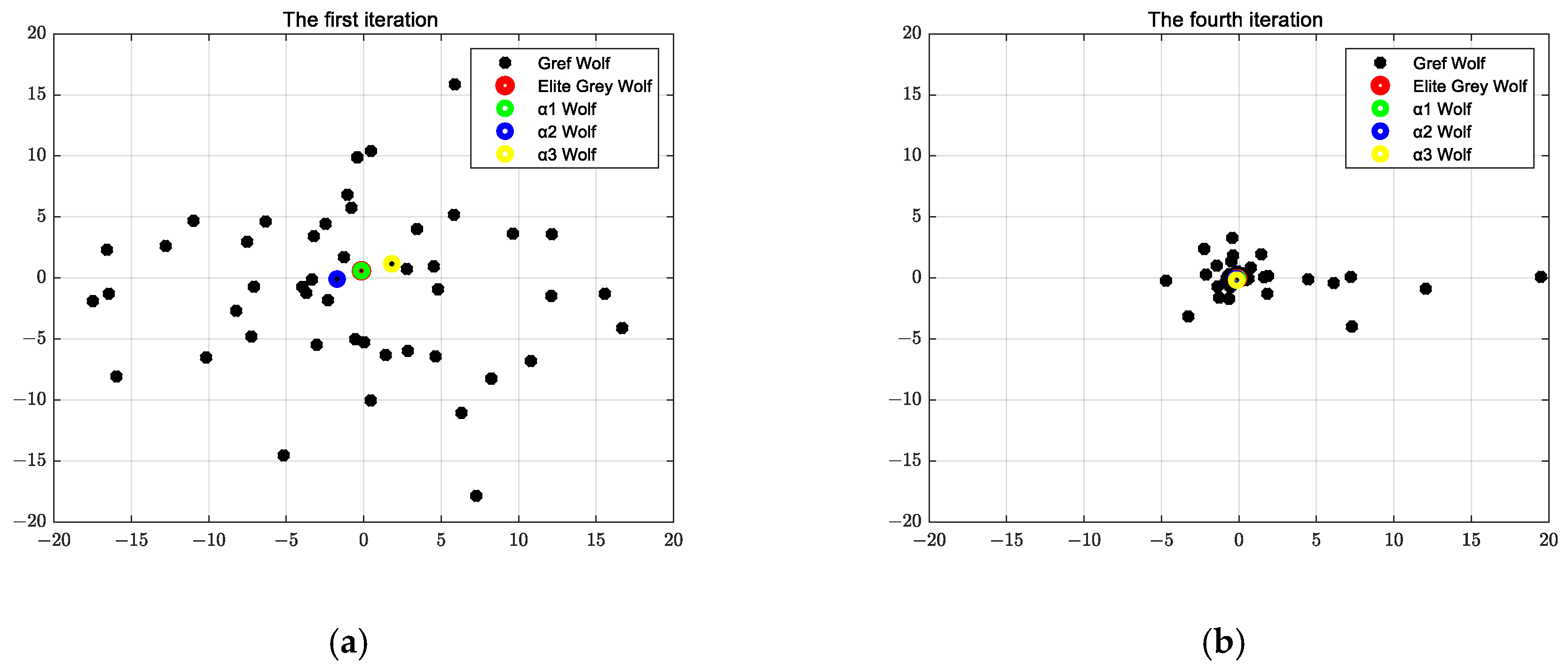
2.3.5. Application of the Grey Wolf Optimization Algorithm

Figure 8 presents the flowchart for the grey wolf optimizer method, outlining the individual steps involved in the calculation. The detailed description of each step is provided below [26].

Step 1: Set the initial values for the maximum iteration count, population size, and variable dimension in the grey wolf optimization algorithm.

Step 2: Randomly assign positions to the members of the grey wolf group within the specified upper and lower bound conditions, based on the real application scenario.

Step 3: Calculate the fitness score for each grey wolf and store the position of the grey wolf with the best (smallest) fitness score as $Y_{{\alpha }_1}$. Retain the position information of a grey wolf with a lower fitness value (sub-optimal) as $Y_{{\alpha }_2}$. Keep the position information of a grey wolf with slightly better fitness value as $Y_{{\alpha }_3}$.

Step 4: Iterate to update the positions of individuals in the pack.

Step 5: Continuously update parameters a, A, and C.

Step 6: Update the ideal positions for three-headed wolves and calculate the fitness values of grey wolves in the pack.

Step 7: Verify whether the maximum number of iterations, t_max, for the optimization algorithm has been reached. If so, use the $Y_{{\alpha }_1}$ value obtained during the optimization process as the best solution. If the maximum number of iterations has not been reached, repeat the process by returning to Step 4.

2.3.6. Grey Wolf Optimization Algorithm Calculation Results

In addition to the aforementioned calculations, the grey wolf optimization technique is employed to tackle the following problems. The objective is to minimize the function value in Formula (8) by finding the optimal values for a pair of variables, x₁ and x₂.

The variables x₁ and x₂ in Formula (8) are constrained within the range of [−20, 20].

The minimum value of this function is 0, and the optimal solution is obtained when x₁ = 0 and x₂ = 0, as indicated by the function expression and the search space depicted in Figure 2. The grey wolf optimization technique can be employed to address this problem. The maximum number of iterations was set to 100, and the population size was 50. The dimension of each individual in the grey wolf population was set to 2, corresponding to the variables x₁ and x₂. The upper boundaries for x₁ and x₂ were both 20, while the lower boundaries were −20 for both variables.

To address the optimization objective, Formula (35) was formulated as the fitness function. The program’s iteration curve is depicted in Figure 9. At the end of the optimization process, the grey wolf optimization algorithm yielded the output values x₁ = −7.7382 × 10⁻³⁶, x₂ = −7.4891 × 10⁻³⁶, and a function value of 6.7313 × 10⁻¹⁴¹, which represents the optimal solution. The obtained value (−7.7382 × 10⁻³⁶, −7.4891 × 10⁻³⁶), as determined by the grey wolf optimization algorithm, was remarkably close to the theoretical optimal value (0, 0). This result serves as evidence of the remarkable optimization capabilities of the grey wolf optimization algorithm.

To gain a better understanding of the distribution of grey wolf individuals in each generation, it is helpful to observe how their positions evolve during the initial and subsequent iterations of the algorithm. Figure 10 provides a visual representation of the shifting positions of individual grey wolves as intermediate results are obtained.

In each generation, it is possible to simultaneously track the best position, also known as the elite grey wolf as well as the overall location of the wolf group. Additionally, the positions of the α₁ wolf, α₂ wolf, and α₃ wolf can be recorded in every generation. As the number of iterations increases, the positions of these wolves gradually converge toward their ideal locations, which in this case is (0, 0). According to the wolf technique, the optimal position (0, 0) can be achieved with a relatively small number of iterations. The grey wolf optimization algorithm demonstrates a tendency to approach its ideal position more closely with each iteration.

When conducting the same number of iterations, the calculation result of the grey wolf optimization algorithm was the most accurate and closest to the ideal position for function $f(x_1,x_2)=x_1{}^4+x_2{}^4$ within the interval of [−20, 20]. It has been demonstrated that the grey wolf optimization algorithm outperforms the wind driven optimization method and the particle swarm optimization algorithm in terms of its strong global optimum ability. Additionally, even with a relatively low number of iterations (10 times), the grey wolf optimization algorithm can achieve a position that is extremely close to the optimal solution while maintaining good computational efficiency. On the other hand, the particle swarm optimization algorithm requires more than 20 iterations, and the wind driven optimization algorithm requires 20 iterations to achieve comparable results.

2.4. One-to-One-Based Optimizer Algorithm

The concept of the one-to-one-based optimizer algorithm (OOBO) revolves around the notion of enhancing the overall knowledge of individuals within the algorithm population. The objective is to strike a balance between maximizing this knowledge and avoiding excessive reliance on particular individuals within a population such as the optimal, average, or worst performers [27]. By establishing a correspondence between two distinct groups of population individuals and selected individuals, the aim is to facilitate greater involvement of all members in the process of updating the algorithm. Moreover, it is crucial to note that each population individual is exclusively chosen as a bootstrap once and solely utilized to update another individual within the population through this one-to-one interaction.

2.4.1. Boundary Range of OOBO Algorithm

Boundary ranges are set for the OOBO algorithm. When the variable exceeds the upper limit, it can only take the value of the upper boundary. When the variable is lower than the lower limit, it can only take the value of the lower boundary. Therefore, the constraint conditions for the particle swarm unit are shown in Equation (36).

$$u_{new}=\left\{\begin{array}{l}ub,u>u_{\max }\\ Ib,u<u_{\min }\end{array}\right.$$

(36)

In Equation (36), ub and Ib represent the upper and lower bounds of the variable, respectively.

2.4.2. Initialization of Parameters of OOBO Algorithm

In the OOBO algorithm, each group member can participate in the solution of this problem. Each member has a mathematical vector representation with the same number of elements as the number of decision variables. A population member can be used as the initial population to generate the OOBO algorithm. Population members are randomly localized in the search space, as shown in Equations (37) and (38).

$$\overrightarrow{X_i}=\{x_{i1},x_{i2},\cdots ,x_{iC},\cdots ,x_{iE}\},i=1,2,\cdots ,M$$

(37)

$$x_{i,C}=I{b}_C+(u{b}_C-I{b}_C)\times rand(),C=1,2\cdots E$$

(38)

2.4.3. Physical Modeling and Population Updating Methods

Individual positions are regularly updated during the optimization seeking procedure using previous heuristic clever optimization algorithms. The method of population update is heavily reliant on the best individual. However, it frequently leads to a loss in the algorithm exploring capabilities. It is easy to fall into a local optimum, making finding a globally optimal solution in the issue space challenging. Moving the population toward the optimal individual may, in fact, lead to convergence to an incorrect local solution for complex optimization problems. Instead of constantly updating the optimization search process with the best individuals, the OOBO algorithm’s modeling design achieves a global search by transferring the algorithm population to different regions of the search space to boost the OOBO searching capabilities. All individuals in the OOBO algorithm are involved in the population update throughout this step. As a result, each population member is chosen at random just once, guiding the search space to produce various results for population.

The OOBO algorithm is described mathematically below.

(1)

Each individual is a positive integer from 1 to N and is chosen randomly.

(2)

Individuals are not duplicated.

(3)

No member has a value equal to its position in the N tuple.

All individuals in the OOBO algorithm are involved in population update throughout this step. As a result, each population member is chosen at random just once, guiding the search space to produce various results for population. As demonstrated in Equation (39), utilize matrix $\overrightarrow{K}$ to bootstrap a set of member locations using aggregate as the stochastic process.

$$\overrightarrow{K}=\{[k_1,\cdots ,k_q,\cdots ,k_N]\in P_{\overline{N}};\forall q\in \overline{N}:k_q\ne q\}$$

(39)

In the above equation, $\overline{N}$ represents the $\{1,2,\cdots ,N\}$ set. $P_{\overline{N}}$ is the arrangement of all $\overline{N}$ sets. In the OOBO algorithm, the process of calculating new states of population members in the search space is modeled, as shown in Equations (40) and (41).

$$x_{i,C}^{new}=\left\{\begin{array}{l}{x}_{i.C}+rand()\cdot (x_{k_i,C}-I{x}_{i,C}),f_{k_i}<f_i\\ x_{i.C}+rand()\cdot (x_{i,C}-x_{k_i,C}),otherwise\end{array}\right.$$

(40)

$$I=round(1+rand())$$

(41)

In the above equation, $x_{i,C}^{new}$ is the new state of the ith individual member in the C dimension. $x_{k_i,C}$ is the ith individual member guided by the selected member under the C dimension. $f_i$ denotes the value of the objective function based on $X_i$. The variable I takes the value of 1 or 2.

A member’s proposed new state is acceptable if it improves the value of the objective function. Otherwise, the proposed new status is rejected, and the individual remains in the existing position. Equation (42) represents the selection process.

$$X_i=\left\{\begin{array}{l}{X}_i^{new},f_i^{new}<f_i\\ X_i,otherwise\end{array}\right.$$

(42)

where $X_i^{new}$ represents the new state of the individual member of the ith population in the search space in the preceding Equation (42). $f_i^{new}$ is the objective function’s value.

2.4.4. Selection of Fitness Function for One-to-One-Based Optimizer

The OOBO optimization algorithm assesses the fitness value of each population member by monitoring changes made to them. The number of unique objective function values recorded in each iteration is equivalent to the number of population members.

2.4.5. Calculation Results of One-to-One-Based Optimizer Algorithm

Combined with the calculation idea of the OOBO algorithm above-mentioned, the OOBO algorithm was used to solve the following problems: solve a group of x₁ and x₂ to minimize the function value as the same as Formula (8).

In Formula (8), the value ranges of x₁ and x₂ were [−20, 20] and [−20, 20], respectively.

From the function expression and search space in Figure 2, the minimum value of this function was 0, and the optimal solution was x₁ = 0 and x₂ = 0. The OOBO algorithm can be used to solve this problem. The population number was 50 and the maximum iteration number was 100. Since x₁ and x₂ were solved, the dimension of individual units was set as 2, the upper boundary of individual units was set as ub = [20, 20], and the lower boundary was set as Ib = [−20, −20].

According to the optimization objective problem, the fitness function designed can be seen in Formula (8). The iteration curve of the program is shown in Figure 11. Finally, the output result of the OOBO algorithm was x₁ = 1.3085 × 10⁻¹⁷, x₂ = 1.2944 × 10⁻¹⁷, and the function value corresponding to optimal solution was 5.7381 × 10⁻⁶⁸. According to the results calculated by the OOBO algorithm, the final value (1.3085 × 10⁻¹⁷, 1.2944 × 10⁻¹⁷) was obviously close to the theoretical optimal value (0, 0). This indicates that the OOBO algorithm has strong optimization ability.

3. Performance Comparison and Study of Various Algorithms

3.1. Descriptive Statistical Analysis

We first wanted to fully compare the performance of four intelligent algorithms: particle swarm optimization (PSO), wind driven optimization (WDO), grey wolf optimization (GWO), and the one-to-one-based optimizer (OOBO). For specific parameters, the population number was set to 100 and the maximum iteration number was set to 1000, as shown in

Table 1. Parameters set by the four algorithms.

Algorithm Name	Set Value of the Algorithm Parameters
Particle Swarm Optimization (PSO)	The population size was set to 100 individuals, the maximum number of iterations was 1000, and the speed range was confined to the interval [−2, 2].
Wind Driven Optimization (WDO)	The population size was set to 100 individuals, the maximum number of iterations was 1000.
Grey Wolf Optimization (GWO)	The population size was set to 100 individuals, the maximum number of iterations was 1000.
One-to-One-Based Optimizer (OOBO)	The population size was set to 100 individuals, the maximum number of iterations was 1000.

.

Benchmark functions (M1–M12) were selected to compare and analyze the performance of the algorithms [28,29], as shown in

Table 2. The unimodal and multimodal experimental test functions (M1–M12).

Test Function	Dimension n	Variables Range	Optimal Solution
$M_1={\displaystyle \sum _{k=1}^n{x}^2{}_k}$	30	[−100, 100]	0
$M_2={\displaystyle \sum _{k=1}^n\left|x_k\right|}+{\displaystyle \prod _{k=1}^n}\left|x_k\right|$	30	[−10, 10]	0
$M_3={\displaystyle \sum _{k=1}^n({\displaystyle \sum _{i=1}^k{x}_i}}{)}^2$	30	[−100, 100]	0
$M_4=\max \left|x_k\right|,(1\le k\le n)$	30	[−10, 10]	0
$M_5={\displaystyle \sum _{k=1}^{n-1}[100{(x_{k+1}-x^2{}_k)}^2+{(x_k-1)}^2]}$	30	[−30, 30]	0
$M_6={\displaystyle \sum _{k=1}^n{(\left|x_k+0.5\right|)}^2}$	30	[−100, 100]	0
$M_7={\displaystyle \sum _{k=1}^{n}k{x}^4{}_k+random(0,1)}$	30	[−1.28, 1.28]	0
$M_8={\displaystyle \sum _{k=1}^n[x_1^2-10\cos (2\pi x_k)+10}]$	30	[−5.12, 5.12]	0
$M_9=-20e^{-0.2\sqrt{\frac{1}{n}{\displaystyle \sum _{k=1}^n{x}_k^2}}}-e^{\frac{1}{n}{\displaystyle \sum _{k=1}^n\cos (2\pi x_k)}}+20+e$	30	[−32, 32]	0
$M_{10}=\frac{1}{4000}{\displaystyle \sum _{k=1}^n{x}_k^2-{\Pi }_{k=1}^n\cos (\frac{x_k}{\sqrt{k}})+1}$	30	[−600, 600]	0
$\begin{array}{l}{M}_{11}=\frac{\pi }{n}\{10\sin (\pi z_1)+{\displaystyle \sum _{k=1}^n{(z_k-1)}^2[1+10\sin (\pi z_{k+1})]}+{(z_n-1)}^2\}\\ +{\displaystyle \sum _{k=1}^{n}U(x_k,10,100,4)}\\ \\ z_k=1+\frac{x_k+1}{4},U(x_k,p,q,r)=\left\{\begin{array}{l}q{(x_k-p)}^r,x_k>p\\ 0,-p<x_k<p\\ q{(-x_k-p)}^r,x_k<-p\end{array}\right.\end{array}$	30	[−50, 50]	0
$\begin{array}{l}{M}_{12}=0.1\{{\sin }^2(3\pi x_1)+{\displaystyle \sum _{k=1}^n{(x_k-1)}^2[1+{\sin }^2(3\pi x_k+1)]+}\\ {(x_n-1)}^2[1+{\sin }^2(2\pi x_n)]\}+{\displaystyle \sum _{k=1}^{n}U(x_k,5,100,4)}\end{array}$	30	[−50, 50]	0

. Unimodal test functions (M1–M7) can be used to evaluate the development ability of intelligent algorithms. The variable dimension of the test function was 30. These functions only contain one global optimal value and are in the form of single peak. Multimodal test functions (M8–M12) have multi-peak forms with a variable dimension of 30. These functions contain multiple local optima and can be used to test the algorithm’s ability to find the global optimum.

In

Table 3. Experimental test functions (M13–M22).

Test Function	Dimension n	Variables Range	Optimal Solution
$M_{13}={[\frac{1}{500}+{\displaystyle \sum _{i=1}^{25}\frac{1}{i+{\displaystyle \sum _{k=1}^2{(x_k-a_{ki})}^6}}}]}^{-1}$	2	[−65, 65]	1
$M_{14}={\displaystyle \sum _{k=1}^{11}{[a_k-\frac{x_1(b_k^2+b_k{x}_2)}{b_k^2+b_k{x}_3+x_4}]}^2}$	4	[−5, 5]	0.0003
$M_{15}=4x_1^2-2.1x_1^4+\frac{1}{3}{x}_1^6+x_1{x}_2-4x_2^2+4x_2^4$	2	[−5, 5]	−1.0316
$M_{16}={(x_2-\frac{5.1}{4{\pi }^2}{x}_1^2+\frac{5}{\pi }{x}_1-6)}^2+10(1-\frac{1}{8\pi })\cos x_1+10$	2	[−5, 5]	0.398
$\begin{array}{l}{M}_{17}=[1+{(x_1+x_2+1)}^2(19-14x_1+3x_1^2-14x_2+6x_1{x}_2+3x_{{}_2}^2)]\\ \times [30+{(2x_1-3x_2)}^2(18-32x_1+12x_1^2+48x_2-36x_1{x}_2+27x_{{}_2}^2)]\end{array}$	2	[−2, 2]	3
$M_{18}=-{\displaystyle \sum _{k=1}^4{d}_k}{e}^{-{\displaystyle \sum _{i=1}^3{p}_{ki}{(x_i-o_{ki})}^2}}$	3	[0, 1]	−3.86
$M_{19}=-{\displaystyle \sum _{k=1}^4{d}_k}{e}^{-{\displaystyle \sum _{i=1}^6{p}_{ki}{(x_i-o_{ki})}^2}}$	6	[0, 1]	-3.32
$M_{20}=-{\displaystyle \sum _{k=1}^5{[(Y-p_k){(Y-p_k)}^T+d_k]}^{-1}}$	4	[0, 10]	−10.1532
$M_{21}=-{\displaystyle \sum _{k=1}^7{[(Y-p_k){(Y-p_k)}^T+d_k]}^{-1}}$	4	[0, 10]	−10.4028
$M_{22}=-{\displaystyle \sum _{k=1}^{10}{[(Y-p_k){(Y-p_k)}^T+d_k]}^{-1}}$	4	[0, 10]	−10.5363

, the M13–M22 test functions are fixed-dimensional multimodal functions [30] that can be used to test the algorithms’ ability to find the global optimum more comprehensively.

In Table 2 and Table 3, each test function (M1–M22) was run 50 times repeatedly. The optimal value, worst value, average fitness value, and standard deviation results were calculated statistically to compare the calculation performance of the four algorithms.

(1)

The optimal value [31]

The ideal value represents the best performance achieved by the algorithms after multiple function tests. When comparing the optimal values obtained by different algorithms after running for the same number of iterations, if one algorithm consistently outperforms the others, it suggests that the algorithm has the ability to discover superior solutions in similar situations.

Equation (43) elegantly formulates the optimal solution that effectively tackles the minimal problem at hand.

$$Optimal Value=\min \{x_1,x_2,x_3,\cdots ,x_n\}$$

(43)

Equation (44) precisely characterizes the optimal solution that effectively resolves the maximum problem under consideration.

$$Optimal Value=\max \{x_1,x_2,x_3,\cdots ,x_n\}$$

(44)

(2)

The worst value [32]

The algorithm’s worst performance can be quantified by the maximum value obtained across multiple test function trials. When subjected to an equal number of iterations, this algorithm consistently yields a higher worst value compared to other algorithms. This observation implies that under identical conditions, this particular algorithm tends to produce inferior solutions.

Equation (45) elegantly formulates the worst solution that effectively tackles the minimal problem at hand.

$$Worst Value=\max \{x_1,x_2,x_3,\cdots ,x_n\}$$

(45)

Equation (46) precisely characterizes the worst solution that effectively resolves the maximum problem under consideration.

$$Worst Value=\min \{x_1,x_2,x_3,\cdots ,x_n\}$$

(46)

(3)

The average value [33]

In the realm of data analysis, the concept of average value serves as a valuable metric in capturing the central tendency of the dataset. This essential statistical measure is computed by summing up all values present in a given dataset and subsequently dividing the sum by the total number of data points. The mathematical formula that articulates this calculation is represented as Formula (47).

$$\overline{X}=\frac{{\displaystyle \sum _{k=1}^n{x}_k}}{n}$$

(47)

Let n denote the total number of data points, and let $\overline{X}$ denote the average value of data. In scenarios where the mean values computed from multiple datasets are all positive, and the optimal solution of the objective function is 0, the dataset with a lower mean value is considered more desirable. Average value serves as a measure of the algorithm’s convergence accuracy.

(4)

The standard deviation [34]

In the domain of mathematics, standard deviation, symbolized by σ, assumes a significant role as it characterizes the dispersion present within a particular dataset. Its definition involves the computation of the arithmetic mean of squared differences between every individual data point and the mean value of the dataset. To mathematically determine standard deviation, one must square deviations, sum them, divide the result by the total number of data points in the set, and ultimately extract the square root. The precise expression of this relationship is elegantly captured in Formula (48).

$$\sigma =\sqrt{\frac{{\displaystyle \sum _{k=1}^n{(x_k-\overline{x})}^2}}{n}}$$

(48)

Let n denote the number of data points, and $\overline{X}$ represent the average value of the dataset. The standard deviation, denoted as σ, provides a measure of dispersion or scatter within the data. A larger standard deviation indicates greater variability in data points, resulting in poorer repetition performance. Conversely, a smaller standard deviation suggests that data points are more closely clustered, leading to better repetition performance.

Table 4. Results obtained from conducting tests on each test function using different algorithms.

Test Function	Algorithm Name	Optimal Value	Worst Value	Average Value	Standard Deviation
M1	PSO	8.80 × 100	1.49 × 101	1.19 × 101	1.42 × 100
	WDO	5.67 × 10−47	1.66 × 10−37	3.42 × 10−39	2.35 × 10−38
	GWO	9.22 × 10−88	2.81 × 10−84	3.11 × 10−85	5.64 × 10−85
	OOBO	1.91 × 10−185	3.01 × 10−183	4.53 × 10−184	0
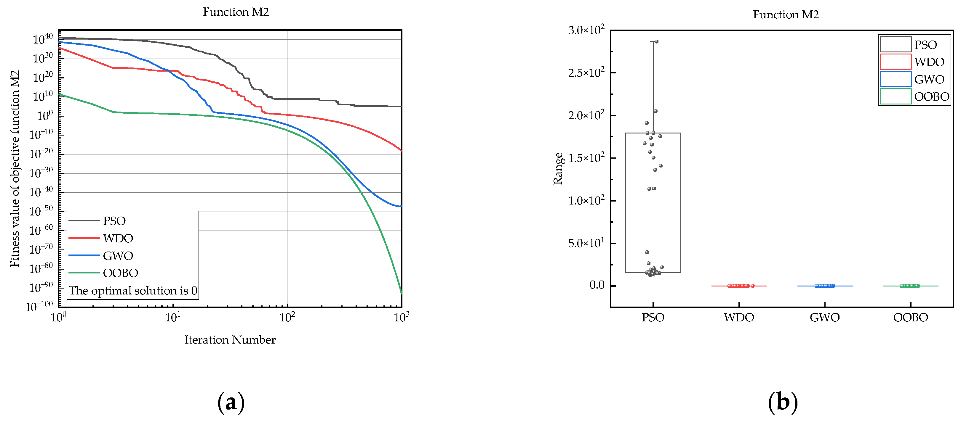
M2	PSO	1.31 × 101	4.57 × 106	1.05 × 105	6.47 × 105
	WDO	4.08 × 10−22	2.45 × 10−17	6.50 × 10−19	3.48 × 10−18
	GWO	4.00 × 10−49	1.90 × 10−47	5.09 × 10−48	4.29 × 10−48
	OOBO	1.49 × 10−94	2.84 × 10−93	7.47 × 10−94	5.19 × 10−94
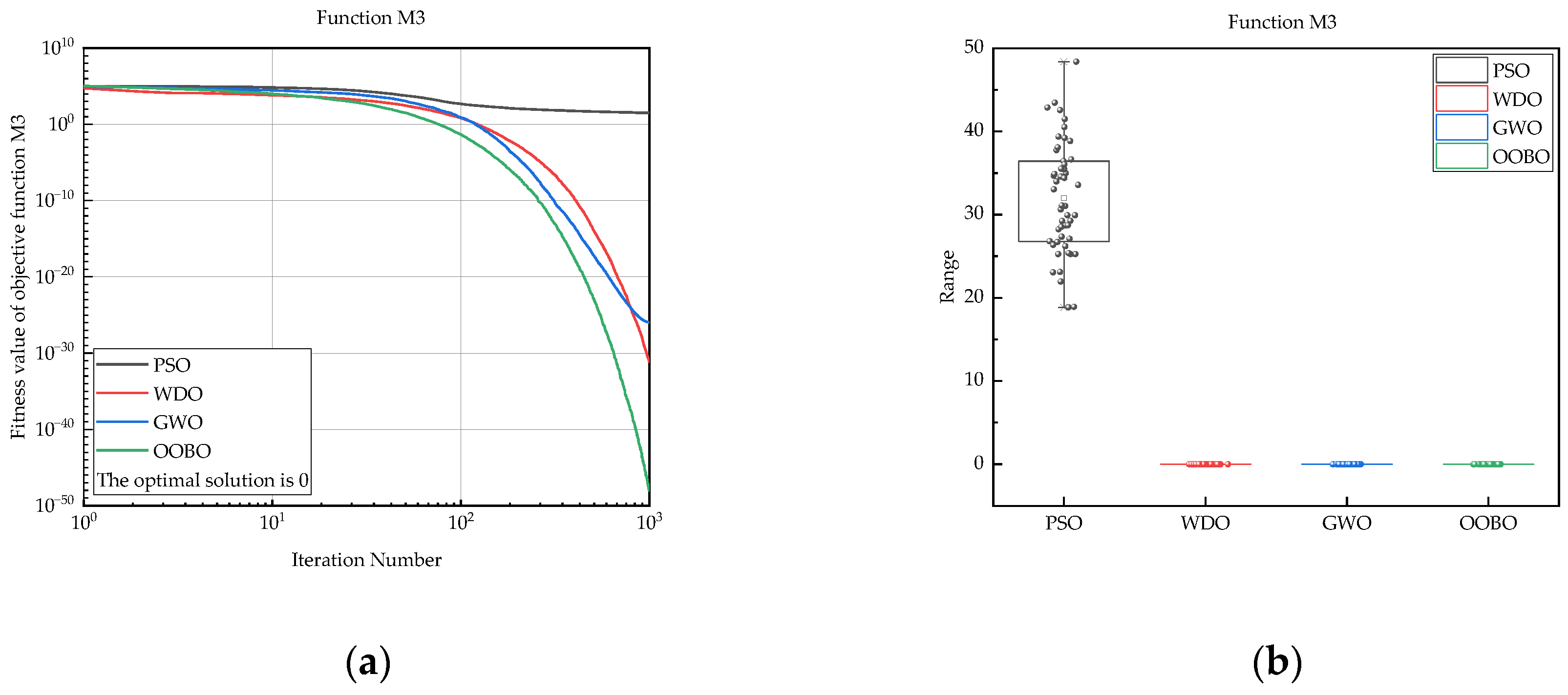
M3	PSO	1.89 × 101	4.84 × 101	3.20 × 101	6.65 × 100
	WDO	9.65 × 10−38	1.84 × 10−30	7.09 × 10−32	2.67 × 10−31
	GWO	4.02 × 10−33	2.57 × 10−25	1.10 × 10−26	4.18 × 10−26
	OOBO	1.45 × 10−57	4.77 × 10−47	9.62 × 10−49	6.74 × 10−48
M4	PSO	1.18 × 100	1.52 × 100	1.36 × 100	7.98 × 10−2
	WDO	1.80 × 10−22	6.05 × 10−18	2.98 × 10−19	9.13 × 10−19
	GWO	2.98 × 10−23	3.53 × 10−21	7.11 × 10−22	7.30 × 10−22
	OOBO	6.04 × 10−79	1.23 × 10−77	5.03 × 10−78	2.99 × 10−78
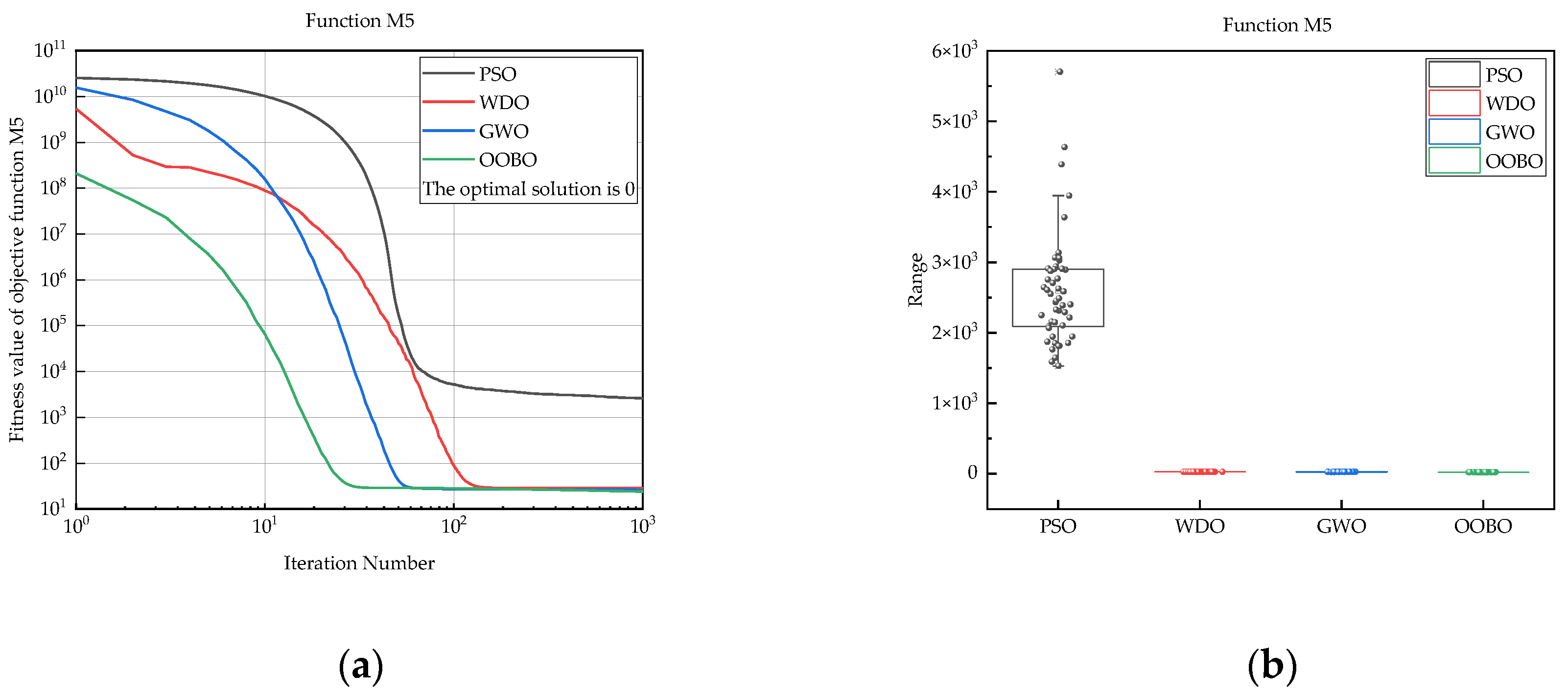
M5	PSO	1.53 × 103	5.70 × 103	2.60 × 103	7.93 × 102
	WDO	2.79 × 101	2.87 × 101	2.84 × 101	3.17 × 10−1
	GWO	2.48 × 101	2.79 × 101	2.63 × 101	7.58 × 10−1
	OOBO	2.30 × 101	2.47 × 101	2.40 × 101	2.17 × 10−1
M6	PSO	7.49 × 100	1.53 × 101	1.19 × 101	1.65 × 100
	WDO	5.41 × 10−2	3.12 × 10−1	1.53 × 10−1	5.77 × 10−2
	GWO	2.05 × 10−6	7.11 × 10−1	1.74 × 10−1	2.01 × 10−1
	OOBO	2.54 × 10−10	1.77 × 10−8	3.65 × 10−9	3.99 × 10−9
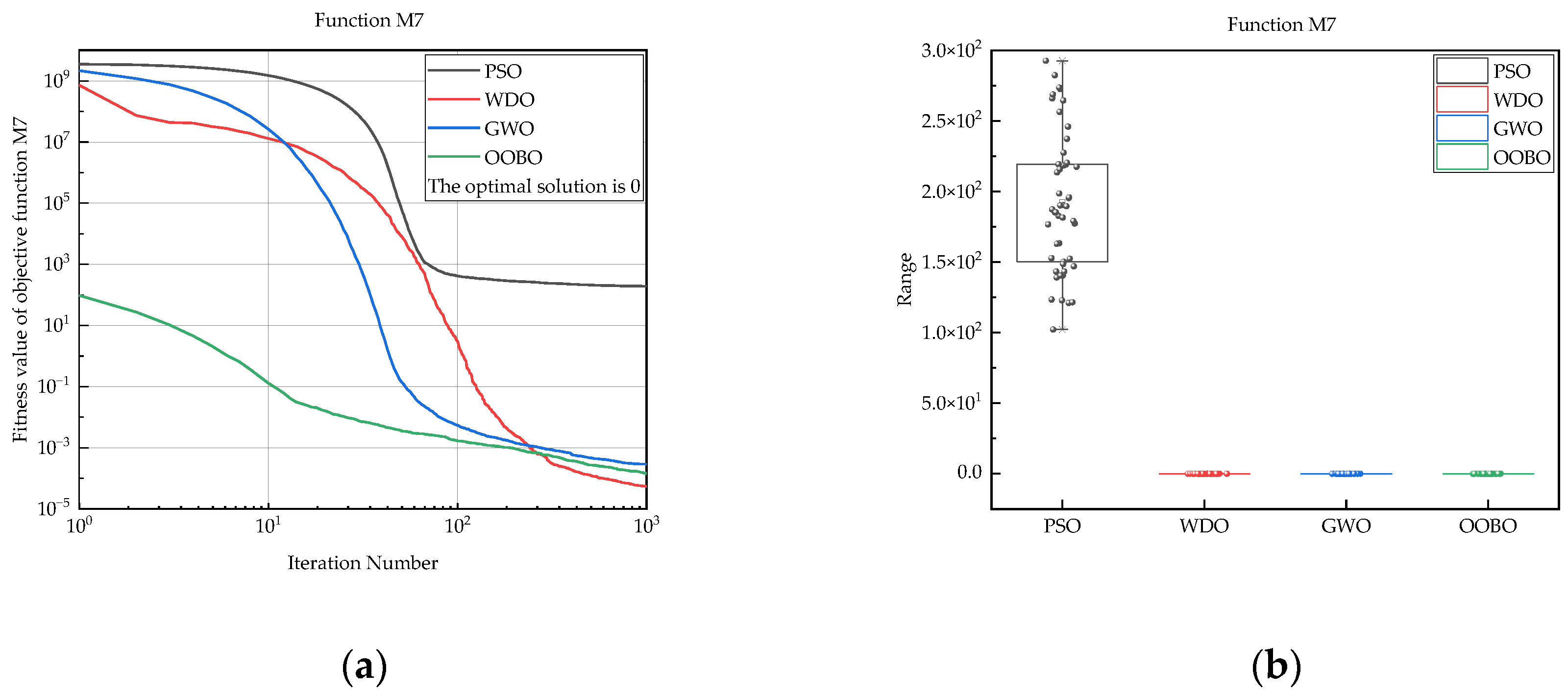
M7	PSO	1.02 × 102	2.93 × 102	1.92 × 102	4.86 × 101
	WDO	9.14 × 10−6	1.50 × 10−4	5.44 × 10−5	3.69 × 10−5
	GWO	4.70 × 10−5	1.10 × 10−3	2.89 × 10−4	1.94 × 10−4
	OOBO	1.95 × 10−5	2.72 × 10−4	1.44 × 10−4	6.59 × 10−5
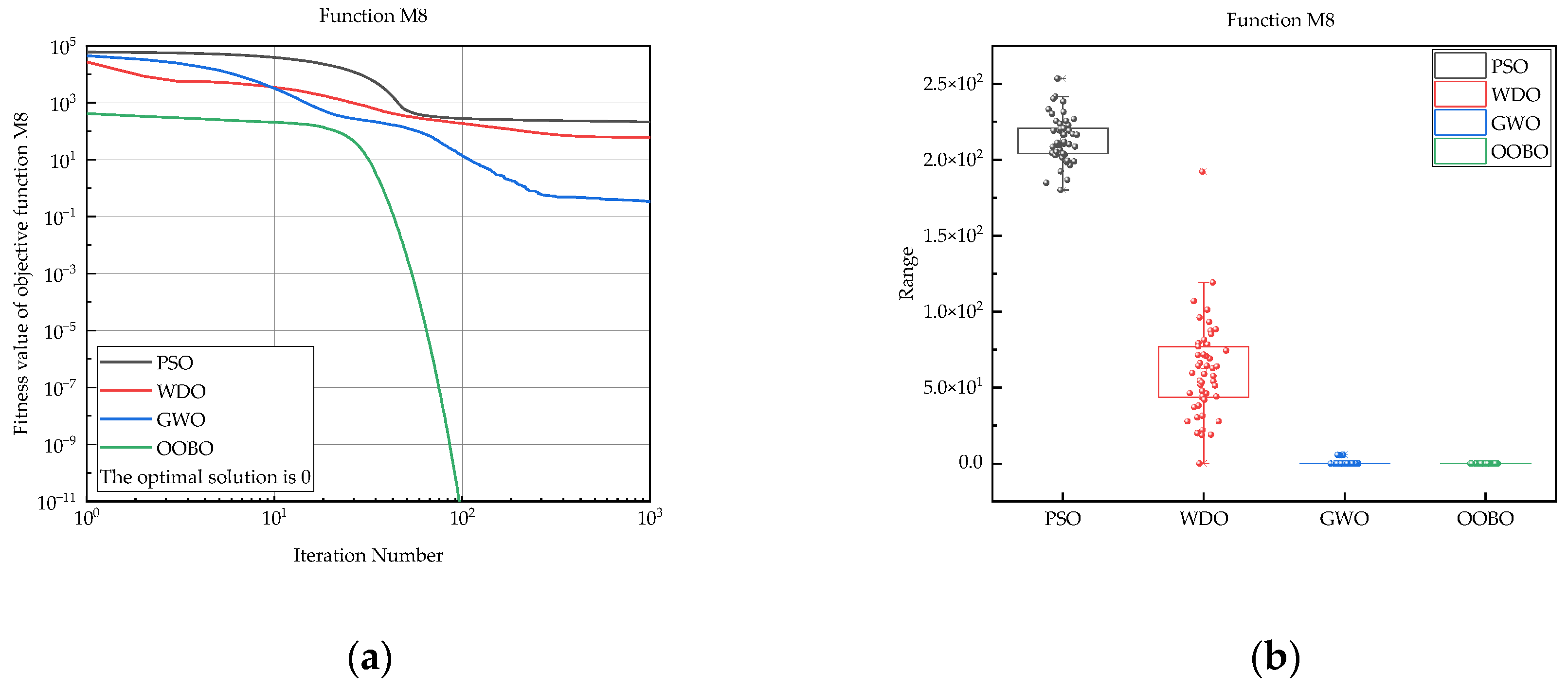
M8	PSO	1.80 × 102	2.53 × 102	2.13 × 102	1.48 × 101
	WDO	0	1.92 × 102	6.07 × 101	3.15 × 101
	GWO	0	5.70 × 100	3.39 × 10−1	1.36 × 100
	OOBO	0	0	0	0
M9	PSO	3.81 × 100	2.10 × 101	1.35 × 101	8.41 × 100
	WDO	0	2.09 × 101	4.19 × 10−1	2.96 × 100
	GWO	2.06 × 101	2.09 × 101	2.08 × 101	7.97 × 10−2
	OOBO	4.00 × 10−15	7.55 × 10−15	4.85 × 10−15	1.53 × 10−15
M10	PSO	3.12 × 10−1	5.87 × 10−1	4.74 × 10−1	4.52 × 10−2
	WDO	0	6.91 × 10−2	2.70 × 10−3	1.04 × 10−2
	GWO	0	1.29 × 10−2	9.00 × 10−4	3.10 × 10−3
	OOBO	0	0	0	0
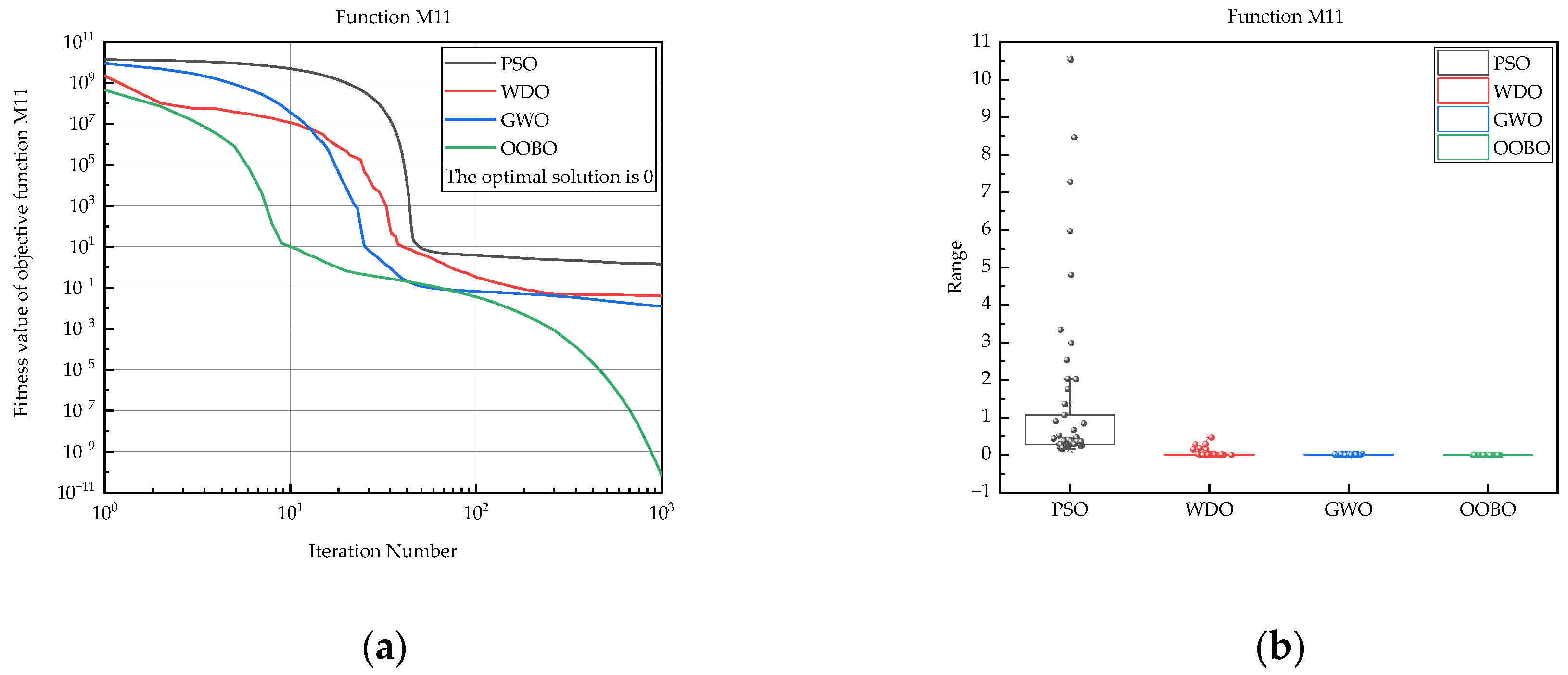
M11	PSO	1.55 × 10−1	1.05 × 101	1.35 × 100	2.26 × 100
	WDO	2.80 × 10−3	4.66 × 10−1	4.03 × 10−2	8.85 × 10−2
	GWO	2.64 × 10−7	3.32 × 10−2	1.27 × 10−2	9.06 × 10−3
	OOBO	1.32 × 10−11	4.44 × 10−10	6.61 × 10−11	6.56 × 10−11
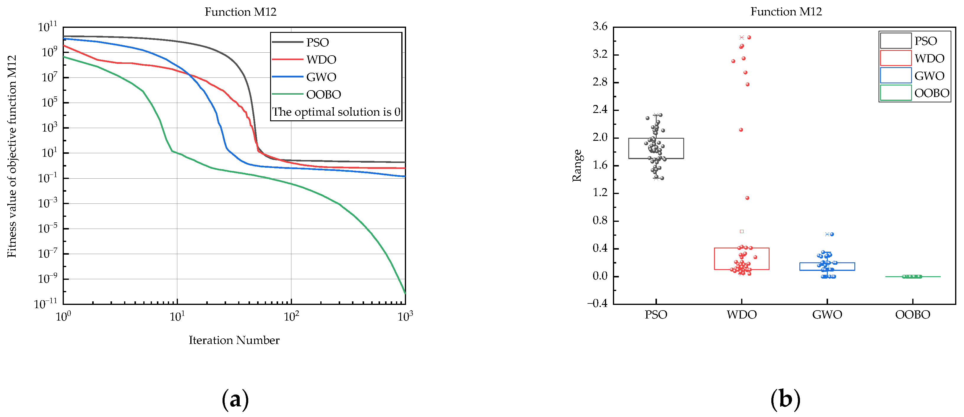
M12	PSO	1.42 × 100	2.33 × 100	1.87 × 100	2.24 × 10−1
	WDO	3.99 × 10−2	3.45 × 100	6.51 × 10−1	1.07 × 100
	GWO	4.18 × 10−6	6.10 × 10−1	1.43 × 10−1	1.22 × 10−1
	OOBO	1.32 × 10−11	4.44 × 10−10	6.61 × 10−11	6.56 × 10−11
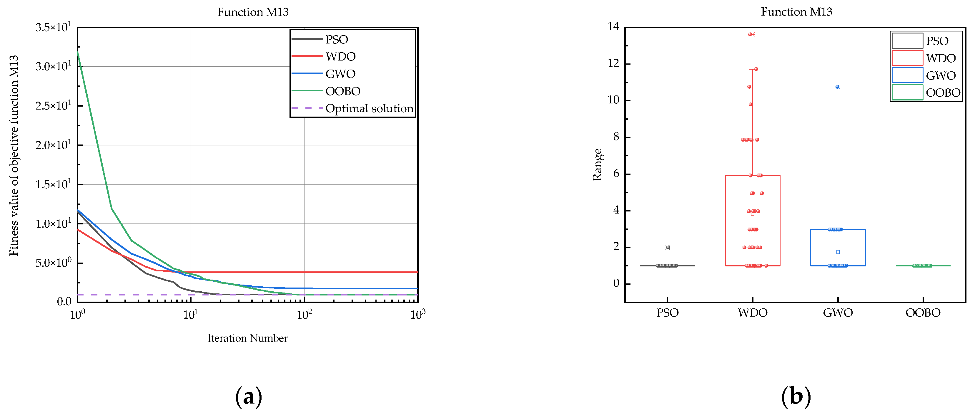
M13	PSO	9.98 × 10−1	1.99 × 100	1.02 × 100	1.41 × 10−1
	WDO	9.98 × 10−1	1.36 × 101	3.83 × 100	3.25 × 100
	GWO	9.98 × 10−1	1.08 × 101	1.75 × 100	1.58 × 100
	OOBO	9.98 × 10−1	9.98 × 10−1	9.98 × 10−1	0
M14	PSO	5.03 × 10−4	1.23 × 10−3	7.89 × 10−4	1.33 × 10−4
	WDO	3.08 × 10−4	2.04 × 10−2	1.20 × 10−3	3.96 × 10−3
	GWO	3.07 × 10−4	5.65 × 10−2	2.25 × 10−3	8.78 × 10−3
	OOBO	3.07 × 10−4	3.07 × 10−4	3.07 × 10−4	4.16 × 10−18
M15	PSO	−1.03 × 100	−1.03 × 100	−1.03 × 100	8.04 × 10−5
	WDO	−1.03 × 100	−1.03 × 100	−1.03 × 100	2.39 × 10−5
	GWO	−1.03 × 100	−1.03 × 100	−1.03 × 100	4.31 × 10−10
	OOBO	−1.03 × 100	−1.03 × 100	−1.03 × 100	2.56 × 10−16
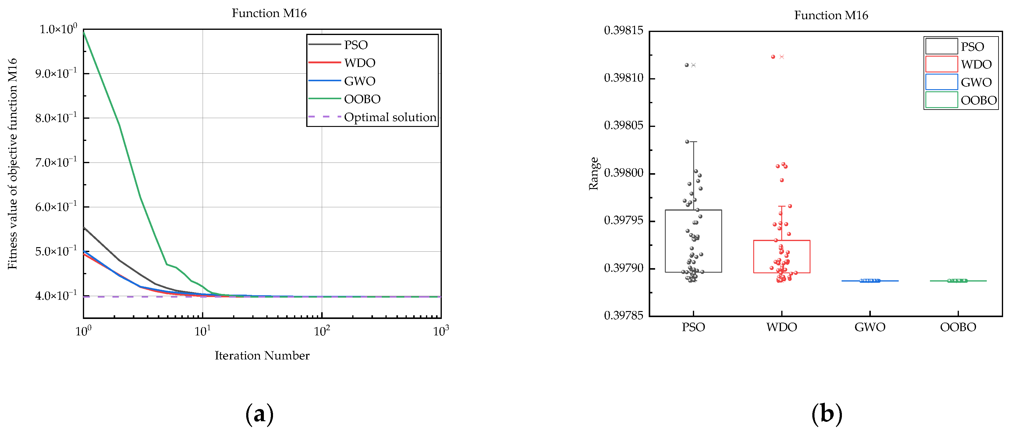
M16	PSO	3.98 × 10−1	3.98 × 10−1	3.98 × 10−1	4.63 × 10−5
	WDO	3.98 × 10−1	3.98 × 10−1	3.98 × 10−1	4.36 × 10−5
	GWO	3.98 × 10−1	3.98 × 10−1	3.98 × 10−1	2.04 × 10−8
	OOBO	3.98 × 10−1	3.98 × 10−1	3.98 × 10−1	0
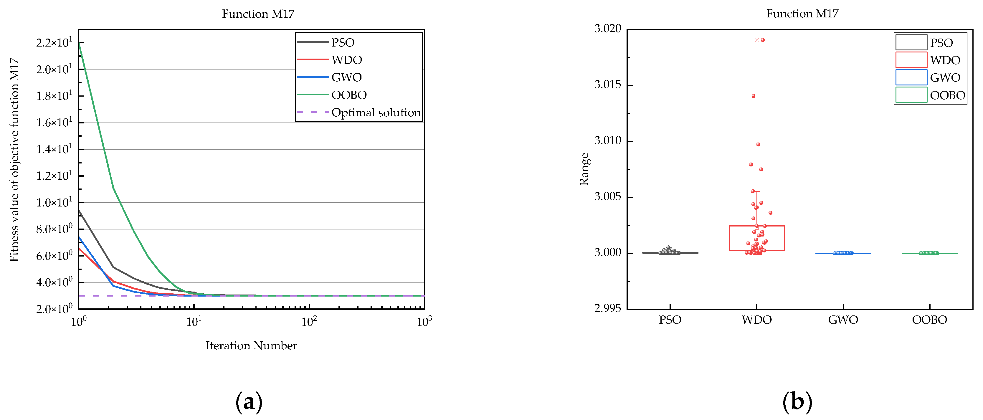
M17	PSO	3.00 × 100	3.00 × 100	3.00 × 100	1.05 × 10−4
	WDO	3.00 × 100	3.02 × 100	3.00 × 100	3.73 × 10−3
	GWO	3.00 × 100	3.00 × 100	3.00 × 100	8.14 × 10−7
	OOBO	3.00 × 100	3.00 × 100	3.00 × 100	5.46 × 10−16
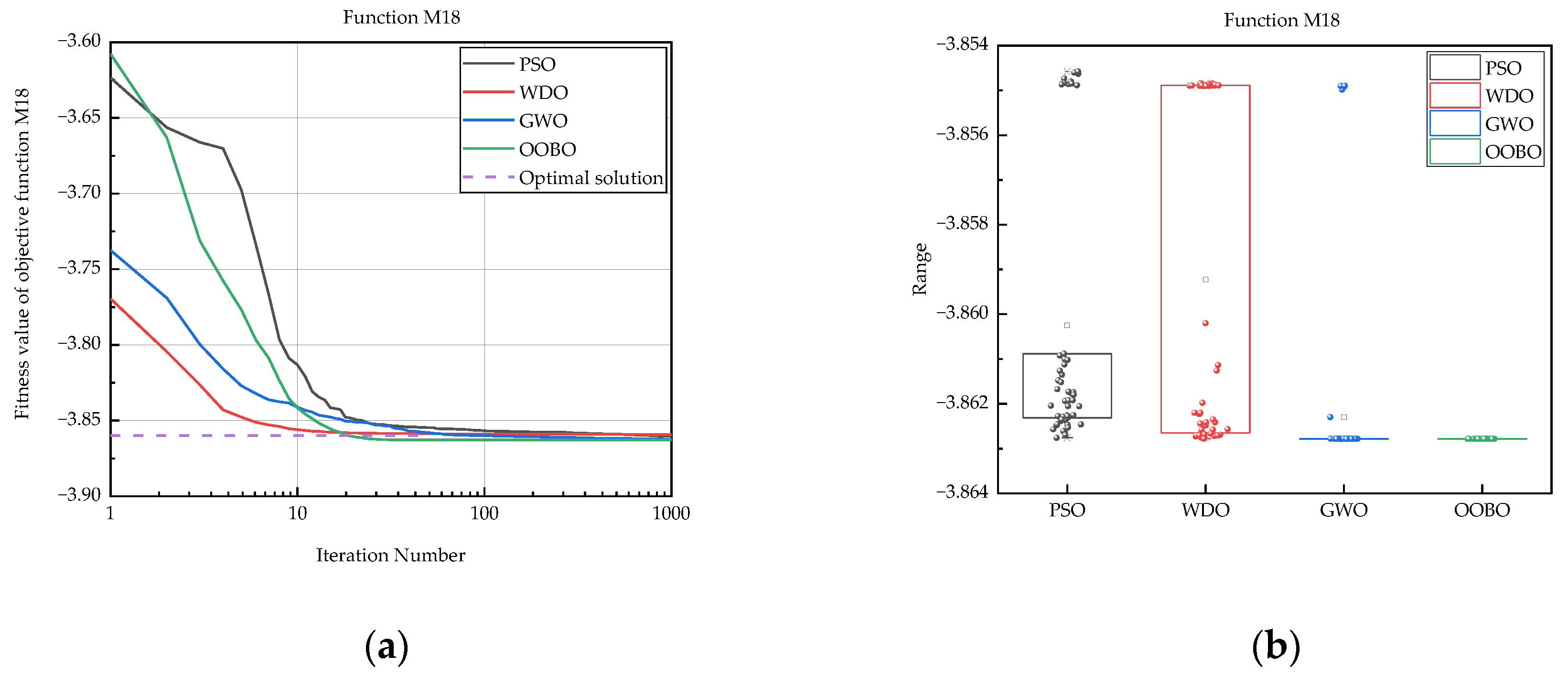
M18	PSO	−3.86 × 100	−3.85 × 100	−3.86 × 100	3.14 × 10−3
	WDO	−3.86 × 100	−3.85 × 100	−3.86 × 100	3.76 × 10−3
	GWO	−3.86 × 100	−3.85 × 100	−3.86 × 100	1.88 × 10−3
	OOBO	−3.86 × 100	−3.86 × 100	−3.86 × 100	1.28 × 10−15
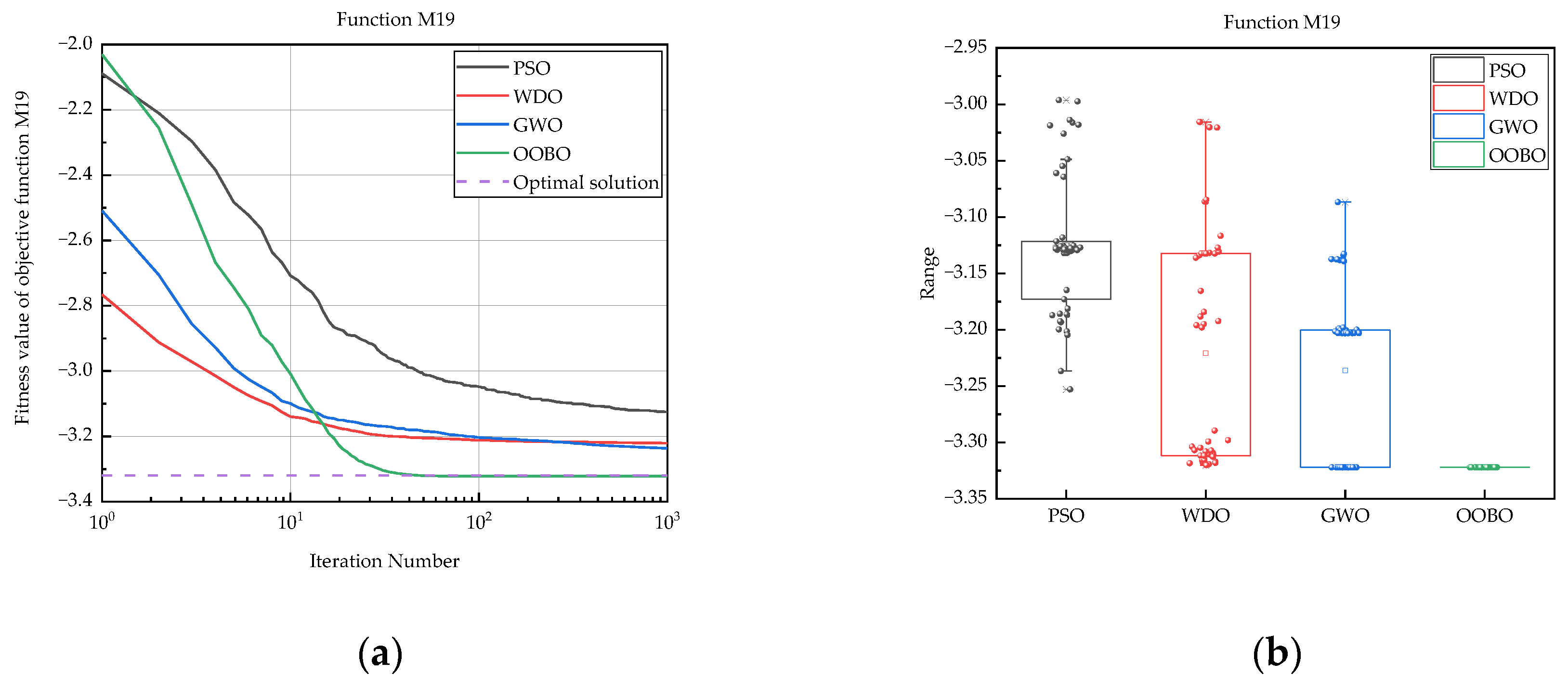
M19	PSO	−3.25 × 100	−3.00 × 100	−3.13 × 100	6.17 × 10−2
	WDO	−3.32 × 100	−3.02 × 100	−3.22 × 100	1.03 × 10−1
	GWO	−3.32 × 100	−3.09 × 100	−3.24 × 100	7.27 × 10−2
	OOBO	−3.32 × 100	−3.32 × 100	−3.32 × 100	9.19 × 10−16
M20	PSO	−1.00 × 101	−2.57 × 100	−7.83 × 100	2.32 × 100
	WDO	−1.00 × 101	−2.43 × 100	−6.78 × 100	2.25 × 100
	GWO	−1.02 × 101	−5.10 × 100	−9.75 × 100	1.38 × 100
	OOBO	−1.02 × 101	−1.02 × 101	−1.02 × 101	3.31 × 10−15
M21	PSO	−1.03 × 101	−2.69 × 100	−8.91 × 100	1.93 × 100
	WDO	−1.02 × 101	−2.73 × 100	−7.21 × 100	2.28 × 100
	GWO	−1.04 × 101	−5.09 × 100	−9.98 × 100	1.46 × 100
	OOBO	−1.04 × 101	−1.04 × 101	−1.04 × 101	1.32 × 10−15
M22	PSO	−1.05 × 101	−5.05 × 100	−9.71 × 100	1.01 × 100
	WDO	−1.04 × 101	−2.24 × 100	−7.66 × 100	2.28 × 100
	GWO	−1.05 × 101	−1.05 × 101	−1.05 × 101	2.30 × 10−5
	OOBO	−1.05 × 101	−1.05 × 101	−1.05 × 101	1.78 × 10−15

Note: The bold results in Table 4 are the minimum values of the three algorithms under different indicators.

presents a comprehensive overview of the performance metrics for various algorithms, specifically their optimal, worst, mean values, and standard deviations. These metrics were obtained by executing 50 independent test functions denoted as M1 to M22. Notably, the most exceptional results achieved by the four distinct algorithms for each test function are highlighted in bold within the table. To gain further insight into the convergence behavior of these algorithms, Figure 12, Figure 13, Figure 14, Figure 15, Figure 16, Figure 17, Figure 18, Figure 19, Figure 20, Figure 21, Figure 22, Figure 23, Figure 24, Figure 25, Figure 26, Figure 27, Figure 28, Figure 29, Figure 30, Figure 31, Figure 32 and Figure 33 visually illustrate the changing patterns of the convergence curves across the test functions (M1–M22).

According to the comprehensive analysis conducted in this study, the convergence curves presented from Figure 12, Figure 13, Figure 14, Figure 15, Figure 16, Figure 17, Figure 18, Figure 19, Figure 20, Figure 21, Figure 22, Figure 23, Figure 24, Figure 25, Figure 26, Figure 27, Figure 28, Figure 29, Figure 30, Figure 31, Figure 32 and Figure 33 as well as the corresponding test results in Table 4, specifically, when considering the unimodal test functions M1–M7, it is evident that the OOBO algorithm exhibited the fastest convergence rate. This conclusion is supported by the observation that the convergence curves of the OOBO algorithm were consistently below those of other algorithms. In other words, at any given moment, the fitness value obtained by the OOBO optimization algorithm was comparatively smaller. Focusing on the performance of the OOBO algorithm in optimizing test functions M1–M6, the final results indicate that the average fitness value achieved by this algorithm was closer to the theoretical optimal value of 0. In contrast, the particle swarm optimization algorithm displayed a tendency to prematurely halt its convergence process, resulting in poor performance. Additionally, the fitness value of the particle swarm optimization algorithm exhibited instability, and the numerical distribution was more discrete in nature. Further analysis considering the optimal value, worst value, and standard deviation results revealed that the OOBO algorithm consistently yielded the smallest values throughout the 50 test iterations. This finding signifies the robustness of the OOBO algorithm in locating the optimum for functions M1–M6. Moreover, the repeatability accuracy of the OOBO algorithm surpassed that of other algorithms. As for the optimization results of test function M7, the wind driven optimization algorithm (WDO) demonstrated the highest level of stability, while the one-to-one-based optimizer (OOBO) was the second-best algorithm in terms of stability.

In the context of multimodal test functions M8–M12, the convergence curves exhibited similarities to those observed in the unimodal test functions. Remarkably, the OOBO optimization algorithm continued to outperform other algorithms, also showcasing its superiority in these scenarios. The convergence speed of the curves became even more pronounced, emphasizing the effectiveness of the OOBO algorithm. In the case of the M8 and M10 functions, the OOBO optimization algorithm displayed an exceptional capability to converge directly to 0, achieving the optimal results. Regarding the M9, M11, and M12 functions, the OOBO algorithm outshone the other algorithms with its remarkable performance. The convergence values attained by the OOBO algorithm were at least four orders of magnitude lower compared to the alternative optimization algorithms, underscoring its unmatched efficacy.

In the study conducted to analyze the performance of various heuristic intelligent optimization algorithms, specifically for test functions M13–M22, it was observed that the OOBO algorithm outperformed other algorithms in terms of convergence speed, convergence optimal value, and result stability. This finding suggests that the OOBO algorithm demonstrates superior capabilities in optimizing these test functions.

Through meticulous analysis of the boxplot diagrams presented in Figure 12, Figure 13, Figure 14, Figure 15, Figure 16, Figure 17, Figure 18, Figure 19, Figure 20, Figure 21, Figure 22, Figure 23, Figure 24, Figure 25, Figure 26, Figure 27, Figure 28, Figure 29, Figure 30, Figure 31, Figure 32 and Figure 33, it is apparent that the optimization outcomes obtained from the OOBO algorithm showcase an exceptional concentration degree and remarkably narrow range. This observation implies that the OOBO algorithm attained the highest level of stability among the examined heuristic intelligent optimization algorithms. Conversely, manifestations of the grey wolf optimization algorithm demonstrated a suboptimal level of stability, whereas the wind driven optimization algorithm manifested a moderately stable behavior. Notably, the particle swarm optimization algorithm exhibited the lowest stability, as evidenced by its wider range of optimization results.

Further analysis revealed that the particle swarm optimization algorithm tended to suffer from premature convergence during the calculation process of test functions, resulting in lower accuracy. The convergence curve of the fitness degree for the particle swarm optimization algorithm was significantly inferior to that of wind driven optimization algorithm, grey wolf optimization algorithm, and one-to-one-based optimizer algorithm. In comparison to the other three optimization algorithms, the particle swarm optimization algorithm was more prone to becoming trapped in the local optima, exhibiting a relatively poor ability to escape from local regions. Conversely, the convergence speed of the grey wolf optimization algorithm experienced a slowdown after approximately 600 iterations in test functions. Similarly, the wind driven optimization algorithm also encountered a deceleration after approximately 50 iterations in the test functions. The convergence curve of the grey wolf optimization algorithm showcased a rapid convergence rate in the initial iterations and demonstrated a commendable ability to escape from local extremums. This can be attributed to the presence of a random variable in the grey wolf optimization algorithm, which assumes a random value within the interval of [0, 2]. The incorporation of this variable influences the wolves’ positional adjustments toward the target prey, facilitating a more randomized search. As a result, the algorithm avoids falling into the local optima during the optimization iteration process [35]. Remarkably, the one-to-one-based optimizer algorithm exhibited the capability to approach the optimal solution when the number of iterations reached about 100.

3.2. Complexity Analysis of Algorithms

In this paper, the computational complexity of the algorithms was focused on analyzing, specifically, in terms of space complexity and time complexity [36]. To investigate this, the average optimization time of three algorithms was compared: particle swarm optimization (PSO), wind driven optimization (WDO), grey wolf optimization (GWO), and one-to-one-based optimizer (OOBO). The analysis was conducted for all four algorithms, and additionally, the average optimization time of GWO in various spatial dimensions were examined. To perform computational analysis, MATLAB R2023a was utilized as the software platform. The hardware configuration of the computer used for analysis consisted of 12th Gen Intel(R) Core (TM) i7-12700H CPU @ 2.30 GHz @ 15.7 GB RAM.

The optimization time of the different algorithms is presented in

Table 5. Total optimization time for the PSO, WDO, GWO, and OOBO algorithms.

Test Function	PSO	WDO	GWO	OOBO
M1	124.84	141.64	252.19	18.21
M2	164.82	189.57	288.32	19.24
M3	83.69	88.55	359.98	46.03
M4	67.19	75.68	252.44	50.33
M5	152.42	170.51	239.31	19.78
M6	52.03	58.68	248.02	39.56
M7	65.53	70.62	295.72	32.71
M8	55.89	61.67	283.99	40.12
M9	54.09	58.45	189.70	17.11
M10	55.59	59.49	286.42	179.16
M11	56.51	61.22	404.10	193.20
M12	301.68	328.69	429.65	377.48
M13	94.61	99.99	88.67	130.31
M14	58.38	70.73	51.73	17.83
M15	27.21	31.41	27.01	17.90
M16	84.24	108.38	63.63	62.39
M17	19.14	22.58	16.75	52.94
M18	50.07	62.08	41.34	18.46
M19	89.01	104.55	83.23	18.73
M20	37.61	42.93	36.26	26.64
M21	27.77	33.27	28.82	23.18
M22	30.88	35.25	32.29	23.83

. The optimization time was measured in seconds. From Table 5, it is evident that the particle swarm optimization algorithm exhibited the shortest optimization time for test functions M10–M13 and M17. The OOBO algorithm takes the least optimization time for test functions M1–M9, M14–M16 and M18–M22. The wind Driven Optimization algorithm and grey wolf optimization algorithm took a longer time to optimize. It was observed that the OOBO algorithm, being a newer heuristic optimization algorithm, possessed superior control capabilities during the optimization process. The calculation process of the OOBO algorithm is simple. Furthermore, the time required to run the algorithm is also related to the number of times the objective function is called during the algorithm optimization.

Table 6. The optimization time in different dimensions.

Test Function	Five Dimensions	Ten Dimensions	Fifteen Dimensions	Twenty Dimensions	Twenty-Five Dimensions	Thirty Dimensions
M1	74.64	132.27	169.67	193.74	212.27	252.19
M2	83.31	140.04	151.74	140.8	247.75	288.32
M3	107.39	154.49	175.64	224.92	312.99	359.98
M4	78.59	120.41	150.56	186.84	250.18	252.44
M5	86.99	144.78	160.22	164.93	172.09	239.31
M6	41.44	129.24	139.13	185.97	190.61	248.02
M7	87.47	87.81	135.67	195.84	204.18	295.72
M8	79.57	97.59	120.83	151.63	236.02	283.99
M9	87.28	94.01	109.18	109.40	184.07	189.70
M10	112.66	140.00	165.53	176.59	270.12	286.42
M11	153.39	176.45	195.9	265.19	324.81	404.10
M12	157.78	214.7	245.1	302.79	393.51	429.65

provides the optimization time required by the grey wolf optimization algorithm in various dimensions for each test function. It can be seen from Table 6 that as the spatial dimension increased, the algorithm progressively faced more challenging optimization tasks, resulting in longer optimization times. The time complexity serves as a metric for quantifying the running time of an algorithm. It is not only evaluated based on the specific calculated time, but can also be expressed by using the O notation, which represents asymptotic complexity. Different algorithms exhibit various forms of time complexity representations such as constant time O(1), linear time O(n), and so on.

Upon analyzing the specific data presented in Table 6, we can provide a detailed analysis of the time complexity of grey wolf optimization algorithm. The GWO algorithm consists of three main components: population initialization, searching for prey (including encircling, pursuing and attacking), and termination judgment. N represents the number of individuals in the initialized wolf population, t denotes the maximum number of algorithm iterations, and n represents the dimension of the space. During the population initialization process, each individual grey wolf’s value is initialized in each dimension, resulting in the time complexity of O(N × n). The process of encircling, pursuing, attacking, and searching for prey within grey wolf population involves nested loops that are dependent on the number of algorithm iterations. Thus, the time complexity of this part of the algorithm involves N, t, and n, resulting in the time complexity of O(t × N × n). The termination judgment process does not involve a loop, resulting in the time complexity of O (1). Therefore, the overall time complexity of the grey wolf optimization algorithm is given by O(t × N × n) + O(N × n) + O(1). Furthermore, the time complexity is influenced by the number of objective functions called during the optimization process. Additionally, the algorithm’s running time is impacted not only by the algorithm itself, but also by the environment in which it operates, the computer hardware performance, programming language, code structure, and other factors.

The space complexity reflects the memory occupied by the algorithm during runtime and serves as an important indicator of its complexity. In the grey wolf optimization algorithm, the number of individuals in the initialized wolf population is N, and the dimension of space is n. Throughout the optimization process, the number of individuals in the wolf population remains constant, and the space dimension is fixed at n. Consequently, the space complexity of the grey wolf optimization algorithm is O(N × n).

3.3. Nonparametric Test Evaluation of Algorithms

When comparing the optimization performance of different heuristic intelligent optimization algorithms across various test functions, there is a lack of a standardized measure, and the presentation of algorithm results may not be visually intuitive. To address this issue, this paper introduced a nonparametric test method known as the Friedman test, which provides an accurate and reliable assessment of the algorithm optimization performance. Nonparametric tests are essential statistical tests that are particularly suitable when the overall distribution of data is unknown or when the assumption of specific distribution is not required. These tests enable a comparison of the overall distributions of multiple samples to determine whether there are any significant differences. The nonparametric test is more flexible and applicable in scenarios involving non-normal and small sample sizes as it has wider range of application and less restriction compared to the parametric test [37].

The Friedman test method is based on the fundamental principle of assigning ranks (sorting) to indicate the relative positions of each sample within each group category. It then calculates the average rank for each group category and determines the presence of significant difference in the overall distribution of samples based on the differences between the rank. The underlying assumption of the Friedman test method is that there is no significant difference in the overall distribution of multiple samples. This assumption can be expressed mathematically as Formula (49).

$$\begin{array}{l}{H}_0:Z_1=Z_2=\cdots Z_n\\ H_1:\exists i,j,Z_i\ne Z_j\end{array}$$

(49)

In Equation (49), Z_i represents the rank ordering of the i sample ($i=1,2,\cdots ,n$), where i represents the number of samples under consideration. The null hypothesis, denoted as H₀, implies that multiple samples are drawn from populations that are not significantly different. On the other hand, H₁ represents the rejection of the null hypothesis, indicating that multiple samples are derived from populations that exhibit significant differences.

The specific steps of the Friedman test method are as follows.

Step 1: First, the ranks of samples in each degree of freedom are calculated. Then, the ranks of the degrees of freedom in each sample are added. For instance, if there are k samples with n freedom degrees to be tested, it can be represented in Equation (50). By arranging data in a matrix form, Equation (51) is obtained.

$$x_{ij}(i=1,2,\cdots ,n;j=1,2,\cdots ,k)$$

(50)

$$X=\left[\begin{array}{ccc}{x}_{11}& \cdots & x_{1k}\\ ⋮& \ddots & ⋮\\ x_{n1}& \cdots & x_{nk}\end{array}\right]$$

(51)

Data groups are sequentially sorted with n degrees of freedom in sample matrix X. That is, first sort $x_{11},\cdots ,x_{1k}$, then sort $x_{21},\cdots ,x_{2k}$, and so on, until the sort $x_{n1},\cdots ,x_{nk}$ is carried out. Finally, n groups of rank data (the number of k in each group) can be obtained, as shown in Equation (52).

$$r_{ij}(i=1,2,\cdots ,n;j=1,2,\cdots ,k)$$

(52)

The rank sum of k samples is seen in Formula (53).

$$R_j={\displaystyle \sum _{i=1}^n{r}_{ij}}(j=1,2,\cdots ,k)$$

(53)

Step 2: Next, we calculate the Friedman statistic. The value of this statistic can be calculated according to Formula (54), containing the rank sum number, the number of freedom degrees, and the number of samples.

$$Y^2=[\frac{12}{nk(k+1)}{\displaystyle \sum _{j=1}^k{R}_j^2}]-3n(k+1)$$

(54)

Step 3: When the sample size is large, it theoretically follows the ${\chi }^2$ distribution of the number of groups minus one, as shown in Equation (55). When the sample size is small (typically less than 40), the results deviate from the ${\chi }^2$ distribution, so a special F-test threshold table can be used to compare with the statistics, as shown in Equation (56).

$$Y^2>{\chi }_{{}_{\theta (k-1)}}^2$$

(55)

$$Y^2>F_{\theta (n,k)}$$

(56)

According to significance level θ, the number of sample groups k, and the number of freedom degrees n, the critical value can be queried. If the calculated statistic is greater than the critical value (or significance level corresponding to statistic is less than the set significance level θ), the null hypothesis H₀ is rejected and hypothesis H₁ is accepted, and the difference of each sample is considered to be significant. Otherwise, the null hypothesis H₀ is accepted and hypothesis H₁ is accepted, and the difference of each sample can be considered as insignificant.

The testing procedure described in the previous section was followed. The hypothesis proposed in this paper based on the Friedman test method is shown in Equation (57).

$$\begin{array}{l}{H}_0:Z_1=Z_2=Z_3\\ H_1:\exists i,j,Z_i\ne Z_j\end{array}$$

(57)

where H₀ represents no significant difference between the four optimization algorithms (PSO, WDO, GWO, OOBO). H₁represents a significant difference between the four optimization algorithms (PSO, WDO, GWO). The average value and standard deviation of the results of the four optimization algorithms described in this paper were sorted independently, the rank was obtained, and then the rank sum of each group’s samples was calculated. As shown in

Table 7. The rank results of the average and standard deviation of the algorithms.

		Average Value			Standard Deviation Value
	Test Function	PSO	WDO	GWO	PSO	WDO	GWO
rij	M1	4	3	2	1	4	3
	M2	4	3	2	1	4	3
	M3	4	2	3	1	4	2
	M4	4	3	2	1	4	3
	M5	4	3	2	1	4	2
	M6	4	2	3	1	4	2
	M7	4	1	3	2	4	1
	M8	4	3	2	1	4	3
	M9	2	4	3	1	4	3
	M10	4	3	2	1	4	3
	M11	4	3	2	1	4	3
	M12	4	3	2	1	3	4
	M13	2	4	3	1	2	4
	M14	2	3	4	1	2	3
	M15	4	3	2	1	4	3
	M16	4	3	2	1	4	3
	M17	4	3	2	1	3	4
	M18	4	3	2	1	3	4
	M19	4	3	2	1	2	4
	M20	4	3	2	1	4	3
	M21	3	4	2	1	3	4
	M22	3	4	2	1	3	4
Rj		35	21	16	34	23	15

, the freedom degree of n was equal to 12 and the sample size k was equal to 4.

The statistical value of the mean and standard deviation for the different algorithms were calculated separately according to Table 7.

$$\mathrm{Average}:Y_1{}^2=\frac{12}{22\times 4\times 5}\times ({80}^2+{66}^2+{51}^2+{23}^2)-3\times 22\times 5=48.71$$

$$\mathrm{Standard} \mathrm{deviation}:Y_2{}^2=\frac{12}{22\times 4\times 5}\times ({77}^2+{68}^2+{50}^2+{25}^2)-3\times 22\times 5=43.04$$

The sample size was small, so it was not suitable to use the ${\chi }^2$ distribution and the Friedman test critical value was used, as shown in

Table 8. The evaluation results of the Friedman test.

Algorithm Name	Sample Size k	Freedom Degree n	Significance Level Set θ	F-Test Critical Value Fθ (n, k)	Statistics Calculated Value
Friedman test result (Average value)	4	22	0.05	5.79	48.71
Friedman test result (Standard deviation value)	4	22			43.04

. The calculated statistic value was greater than the critical value, so null hypothesis could be rejected at a significance level of 0.05. Four algorithms (PSO, WDO, GWO, and OOBO) were significantly different.

In addition,

Table 9. The optimization results in rank-mean ordering with the mean and standard deviation.

	PSO	WDO	GWO	OOBO
Mean-rank ordering (Mean)	3.64	3.00	2.32	1.04
Mean-rank ordering (Standard deviation)	3.50	3.09	2.27	1.14

shows that the rank mean of the OOBO algorithm was the smallest in terms of the mean and standard deviation of the optimization results for the different algorithms. Combined with the results of the three algorithms in Table 4 after optimizing 22 test functions, 50 times, it can be found that the OOBO algorithm had the largest amount of data highlighted in bold. In conclusion, compared with the other optimization algorithms, the OOBO algorithm had the best algorithm optimization ability.

3.4. Algorithmic Control Parameters Effect on Results

In this section, the particle swarm optimization algorithm was delved to elucidate the impact of the algorithm control parameters on the heuristic intelligent optimization outcomes. Based on the previous exposition on the particle swarm optimization algorithm, it can be ascertained that the optimization efficacy of the algorithms is contingent upon several factors including but not limited to the number of populations, particle dimensions, iteration counts, inertia weights, and learning factors. These considerations play a crucial role in influencing the overall performance of the algorithms.

In the context of the particle swarm optimization algorithm, the parameter denoting the number of population M assumes the paramount importance. It is worth noting that a smaller population size renders the algorithm susceptible to local optimization, whereby suboptimal solutions are obtained. Conversely, a larger population size facilitates the enhanced convergence of the optimization curve, enabling algorithms to swiftly converge upon the global optimal solution. However, it is imperative to consider that an augmented population size amplifies the computational burden per iteration. Beyond a certain threshold, augmenting the population size yields diminishing returns [38]. To navigate this trade-off effectively, it is recommended to select a population size from the range of values [20, 1000]. For simpler problems, a population size of 20–100 is generally deemed appropriate, whereas more intricate or class-specific problems necessitate a population size of 100–1000.

The particle dimension E represents the dimension of the particle search space, and this parameter is related to the space in which the actual problem is solved.

The number of iterations, denoted as Q, signifies the frequency at which the heuristic intelligent optimization algorithm executes. If the number of iterations is too limited, it may lead to unstable solution outcomes. Conversely, an excessively large number of iterations will result in a time-consuming solution process, yielding only marginal improvements to the final result [39]. Consequently, it is crucial to adjust the number of iterations based on the specific circumstances of optimization calculation. The recommended range for the number of iterations is typically between 50 and 100, with exemplary values such as 60, 70, and 100. By analyzing the iteration patterns of various algorithms on distinct test functions, it becomes apparent that when the number of iterations approaches approximately 100, the solutions converge significantly toward the desired target.

Researchers Yuhui Shi and Russell Eberhart [40] introduced the notion of the inertia coefficient w within the elementary particle swarm algorithm. Their proposal involves dynamically adjusting this coefficient to achieve a balance between the global convergence capabilities and convergence speed [41]. The inertia coefficient plays a vital role in determining the impact of the particle velocities of the previous generations on the current velocities. Essentially, it reflects the level of confidence particles have in their current motion state and influences their inertial movements based on their own velocities. By preserving the inertia of motion and promoting an inclination for exploring an extended solution space, the particle is able to strike a harmonious balance between global exploration and local convergence. The magnitude of the inertia coefficient directly influences the particle’s ability to explore novel regions, thus affecting its global optimization capabilities. A higher inertia coefficient value enhances the particle’s capacity to traverse unexplored territories, thereby bolstering its global optimization prowess. However, this comes at the expense of weaker local optimization abilities. Conversely, a lower inertia coefficient value strengthens the particle’s proficiency in a local search, facilitating faster convergence toward the optimal solution. Larger inertia coefficient values are particularly advantageous for conducting a global search, enabling particles to venture beyond the local optima and avoid being trapped within them. On the other hand, smaller inertia coefficient values excel at a local search, facilitating rapid convergence to an optimal solution. When confronted with a vast problem search space, it is essential to strike a balance between the search speed and search accuracy. In such cases, optimization algorithms can be designed to emphasize high global search abilities during the initial stages in order to obtain suitable particles. Subsequently, in later stages, greater emphasis can be placed on local search capabilities to enhance the convergence accuracy [42]. By adopting this approach, a harmonious trade-off between the search speed and search accuracy can be achieved, leading to superior optimization outcomes in a complex search space.

When w is 1, the algorithm is an elementary particle swarm algorithm. When w is 0, particles themselves loses the thought of experience. The recommended range of values for the inertia coefficient is [0.4, 2], with typical values such as 0.9, 1.2, 1.5, and 1.8.

In the context of optimization problems for practical engineering applications, it is common to employ a two-step approach: a global search followed by a local fine search. This strategy allows the search space to converge swiftly to a specific region using the global search, and subsequently, a local fine search can be conducted to obtain a highly accurate solution. To enhance the algorithm’s adaptive ability, an adaptive tuning strategy can be implemented, which involves linearly reducing the value of the inertia coefficient as the iterations progress. The adjustment of the inertia coefficient, as depicted in Equation (58) of this paper, follows a linear change strategy commonly employed in such scenarios. Specifically, the inertia coefficient decreases with an increase in the number of iterations [43]. This approach endows the particle swarm optimization algorithm with a robust global convergence ability during the initial stage, and a potent local convergence ability during the later stage. Consequently, the algorithm’s searching adaptive ability is significantly improved. By incorporating this adaptive tuning strategy, the particle swarm optimization algorithm becomes more effective in solving optimization problems for practical engineering applications.

$$w=w_{\max }-(w_{\max }-w_{\min })\frac{Q}{Q_{\max }}$$

(58)

The learning factors, c₁ and c₂, play a crucial role in the particle swarm optimization algorithm. Formula (5) provides insight into their significance. Specifically, c₁ represents the influence of an individual particle’s own experience, guiding it toward its personal optimal position. On the other hand, c₂ represents the impact of the collective experience of other particles, encouraging the particle to move toward the group’s optimal position. When c₁ is set to 0, the algorithm becomes a selfless particle swarm algorithm, prioritizing the collective welfare over individual gains. This may lead to a rapid loss in group diversity, making the algorithm susceptible to becoming trapped in the local optima and restricting its ability to escape. Conversely, setting c₂ to 0 transforms the algorithm into a self-cognizant particle swarm algorithm, emphasizing individual exploration without any social information sharing. Consequently, convergence of the algorithm becomes slow due to the absence of collaborative learning. To strike a balance between individual and collective learning, it is recommended to set both c₁ and c₂ to non-zero values, forming a complete particle swarm algorithm. This choice enables the algorithm to maintain a reasonable convergence speed while preserving an effective search capability. It is important to note that setting learning factors too low may cause particles to remain outside the target area, while excessively high values may result in particles crossing the target area directly [44]. Learning factors typically fall within the range of [0, 4], with commonly employed values like c₁ = c₂ = 2, c₁ = 1.6, c₂ = 1.8, or c₁ = 1.6, c₂ = 2. These values strike a balance between individual and social learning, facilitating efficient convergence and effective search performance.

The above analysis of factors affecting the particle swarm optimization algorithm shows that a variety of factors can affect the results of the particle swarm optimization algorithm. Upon the identification of a research problem requiring resolution, it becomes imperative to determine the particle dimension, followed by setting appropriate values for the number of populations, iterations, inertia coefficient, and learning factor. Notably, the distinct values assigned to these parameters will invariably influence the outcome of the algorithmic optimization process. In the research conducted by Liu Xinwei [45], the influence of particle population parameters including the population number, inertia coefficient, learning factor, and velocity correlation coefficient on the simulation results of the Xin’anjiang River water conservancy model was studied. Five different levels were considered for each parameter, and an L₂₅(5⁶) orthogonal table was applied to design the orthogonal test. The test results were analyzed to determine the effects of these parameters on the performance of the particle swarm optimization algorithm in this model. Additionally, the optimal parameter combination scheme was derived. This finding highlights the importance of selecting appropriate values for the population size and inertia coefficient when using the particle swarm optimization algorithm in this specific model. Another study conducted by Liu Zhixiong [46] focused on continuous function optimization problems and job shop scheduling problems. Researchers controlled the random parameter variables using the particle swarm optimization algorithm and performed experimental analysis. These results demonstrated that setting different values for random number parameters such as the number of populations, particle dimensions, and iterations in the particle swarm optimization algorithm significantly influenced its optimization performance. Overall, these studies emphasize the need to carefully select and configure the particle swarm optimization algorithm’s parameters to achieve the optimal results in various applications.

Through the aforementioned analysis presented in this research article, it is evident that the particle swarm optimization algorithm’s selection of different control parameters exerts a substantial influence on the optimization outcomes. When a specific research target is established, the number of particle dimensions can be determined, resulting in the recommended range of controlling the number of populations within [20, 1000]. Similarly, the number of iterations should be confined to [50, 100]. By employing a linear variation strategy, the inertia factor can be modulated within the interval [0.4, 2], whereas the learning factor is advised to be set between [0, 4]. In order to address practical application problems, it is suggested to employ heuristic intelligent optimization algorithms as referenced in the literature [45,46]. By employing an orthogonal test design, it becomes possible to identify influential parameter combinations and subsequently analyze the optimization outcomes associated with different combinations. Subsequently, an optimal parameter combination scheme can be derived to enhance the overall effectiveness of the optimization process.

4. Conclusions

The study investigated four heuristic intelligent optimization algorithms and employed a set of twenty-two test functions, comprising seven unimodal test functions, five multimodal test functions, and ten mixed combination test functions. The objective was to analyze and evaluate the algorithms’ performance from four perspectives: descriptive statistics analysis, algorithm complexity, nonparametric statistics, and influence of algorithmic parameters on results. The evaluation results were subsequently presented. Ultimately, this paper is concluded by summarizing the key characteristics of heuristic intelligent optimization algorithms.

By examining the particle swarm optimization algorithm, wind driven optimization algorithm, grey wolf optimization algorithm and one-to-one-based optimizer algorithm, it becomes evident that heuristic intelligent optimization algorithms can be dissected into the following stages from a computational standpoint: population initialization and updating, the establishment of target fitness functions, and the verification of boundary constraint conditions. These algorithms share several common traits, namely each agent is represented by multiple particles, individuals within a population possess a relative sense of independence, solution space exploration occurs through positional changes governed by specific rules, and the addition of random numbers enhances the comprehensiveness of the search process.

In terms of the final average convergence values, the one-to-one-based optimizer algorithm had the lowest optimization result in single-peak test functions M1–M6. The wind driven optimization algorithm had slightly lower results than the one-to-one-based optimizer algorithm in single-peak test function M7. For multi-peak test functions M8–M12 and combined hybrid test functions M13–M22, the one-to-one-based optimizer algorithm had significantly smaller result values than the other algorithms. Combined with the perspectives of stability and convergence speed, the one-to-one-based optimizer algorithm had the best performance compared to other heuristic intelligent optimization algorithms.

Algorithm complexity encompasses two crucial factors regarding space complexity and time complexity. When it comes to the wind driven optimization algorithm and grey wolf optimization algorithm, their time complexities were notably high, and is contingent upon the number of individuals, maximum iteration count, and space dimension. On the other hand, the space complexity of an algorithm is influenced by the number of individuals and the space dimension. It is worth noting that as the space dimension expands, the algorithm’s time complexity will experience an increase. The time complexity and space complexity of the particle swarm optimization algorithm and the one-to-one-based optimizer algorithm were comparatively small. The one-to-one-based optimizer algorithm had the best performance.

In this paper, the Friedman test method of nonparametric statistics was used by introducing parametric statistics and comparing them with statistics under the assumed significance level. It was found that there were significant differences between the particle swarm optimization algorithm, wind driven optimization algorithm, grey wolf optimization algorithm and one-to-one-based optimizer algorithm. At the same time, combined with the nonparametric test results of the mean and standard deviation, the performance of one-to-one-based optimizer algorithm was evaluated to be the best.

The results of the heuristic intelligent optimization algorithm solution are not necessarily for all optimal solutions. It may be one of the local optimal solutions, resulting in falling into the local optimum value. Although the current development of heuristic intelligent optimization algorithms is rapid, the control parameters selected by the algorithms are different for optimization problems in various application contexts. Therefore, specific problems need to be treated with specific analysis.

References

- Yu, J.; Zhou, X.; Chen, M. Research on Representative Algorithms of Swarm Intelligence. Comput. Eng. Appl. 2010, 46, 1–4+74. [Google Scholar]
- Xie, L.; Zheng, Y.; Chen, J. Enabling Technologies in the Problem Solving Environment HED. Commun. Comput. Phys. 2008, 4, 1170–1193. [Google Scholar]
- Kennedy, J.; Eberhart, R. Particle Swarm Optimization. In Proceedings of the ICNN ‘95—International Conference on Neural Networks, Perth, WA, Australia, 27 November–1 December 1995. [Google Scholar]
- Shi, Y.; Eberhart, R. A Modified Particle Swarm Optimizer. In Proceedings of the 1998 IEEE Congress on Evolutionary Computation, Anchorage, AK, USA, 4–9 May 1998; pp. 69–73. [Google Scholar]
- Shi, Y.; Eberhart, R. Empirical Study of Particle Swarm Optimization. In Proceedings of the 1999 IEEE Congress on Evolutionary Computation, Washington, DC, USA, 6–9 July 1999; pp. 1945–1950. [Google Scholar]
- Chen, W.; Wu, X. Improved Wind Driven Optimization Algorithm Based on Multi-Strategy Fusion. J. Chongqing Univ. Sci. Technol. (Nat. Sci. Ed.) 2022, 24, 44–52. [Google Scholar]
- Gu, Q.; Zhang, S.; Liu, S. Application of an Improved Wind Driven Optimization Algorithm in Reservoir Operation. J. China Inst. Water Resour. Hydropower Res. 2022, 20, 237–243+250. [Google Scholar]
- Zhang, S.; Luo, Q.; Zhou, Y. Hybrid Grey Wolf Optimizer Using Elite Opposition-Based Learning Strategy and Simplex Method. Int. J. Comput. Intell. Appl. 2017, 16, 1750012. [Google Scholar] [CrossRef]
- Kong, X.; Yao, Y.; Yang, W.; Yang, Z.; Su, J. Solving the Flexible Job Shop Scheduling Problem Using a Discrete Improved Grey Wolf Optimization Algorithm. Machines 2022, 10, 1100. [Google Scholar] [CrossRef]
- Chen, M.; Chen, J.; Zeng, G. An Improved Artificial Bee Colony Algorithm Combined with Extremal Optimization and Boltzmann Selection Probability. Swarm Evol. Comput. 2019, 49, 158–177. [Google Scholar] [CrossRef]
- Lee, K. Modern Heuristic Optimization Techniques with Applications to Power Systems; John Wiley & Sons: Hoboken, NJ, USA, 2005. [Google Scholar]
- Yang, W.; Li, Q. Survey on PSO Algorithm. Eng. Sci. 2004, 6, 87–94. [Google Scholar]
- Bergh, F.; Engelbrecht, A. A Study of PSO Particle Trajectories. Inf. Sci. 2006, 176, 937–971. [Google Scholar]
- Chen, Q.; Zheng, Y.; Jiang, H. Improved Particle Swarm Optimization Algorithm Based on Neural Network for Dynamic Path Planning. J. Huazhong Univ. Sci. Technol. (Nat. Sci. Ed.) 2021, 49, 51–55. [Google Scholar]
- Liu, H.; Zeng, H.; Zhou, W. Optimization of Job Shop Scheduling Based on Improved Particle Swarm Optimization Algorithm. J. Shandong Univ. (Eng. Sci.) 2019, 49, 75–82. [Google Scholar]
- Chatterjee, A.; Siarry, P. Nonlinear Inertia Weight Variation for Dynamic Adaptation in Particle Swarm Optimization. Comput. Oper. Res. 2006, 33, 859–871. [Google Scholar] [CrossRef]
- Spavieri, G.; Cavalca, D.; Fernandes, R. An Adaptive Individual Inertia Weight Based on Best, Worst and Individual Particle Performances for the PSO Algorithm. In Proceedings of the 17th International Conference on Artificial Intelligence and Soft Computing, ICAISC 2018, Zakopane, Poland, 3–7 June 2018; pp. 536–547. [Google Scholar]
- An, P. Particle Swarm Optimization Algorithm Based on Chaotic Theory and Adaptive Inertia Weight. J. Nanoelectron. Optoelectron. 2017, 12, 404–408. [Google Scholar]
- Bayraktar, Z.; Komurcu, M.; Werner, D. Wind Driven Optimization (WDO): A Novel Nature-inspired Optimization Algorithm and Its Application to Electromagnetic. In Proceedings of the Antennas and Propagation Society International Symposium (APSURSI), Toronto, ON, Canada, 11–17 July 2010; pp. 1–4. [Google Scholar]
- Ren, Z.; Zhang, R.; Tian, Y. Wind Driven Optimization Algorithm. J. Jiangsu Univ. Sci. Technol. (Nat. Sci. Ed.) 2015, 29, 153–158. [Google Scholar]
- Yanxia, S.; Chikomborero, S.; OdunAyo, I. OFDM Network Optimization Using a QPSK Based on a Wind-Driven Genetic Algorithm. Sensors 2022, 22, 6174. [Google Scholar]
- Ranjan, P. The Synthesis of a Pixelated Metamaterial Cross-polarizer Using the Binary Wind-driven Optimization Algorithm. J. Comput. Electron. 2022, 21, 453–470. [Google Scholar] [CrossRef]
- Seyedali, M.; Seyed, M.; Andrew, L. Grey Wolf Optimizer. Adv. Eng. Softw. 2014, 69, 46–61. [Google Scholar]
- Zhang, X.; Wang, X. Comprehensive Review of Grey Wolf Optimization Algorithm. Comput. Sci. 2019, 46, 30–38. [Google Scholar]
- Ahmed, H.; Youssef, B.; Eikorany, A. Hybrid Grey Wolf Optimizer-artificial Neural Network Classification Approach for Magnetic Resonance Brain Images. Appl. Opt. 2018, 57, 25. [Google Scholar] [CrossRef]
- Li, S.; Ye, C. Improved Grey Wolf Optimizer Algorithm Using Nonlinear Convergence Factor and Elite Re-election Strategy. Comput. Eng. Appl. 2021, 57, 62–68. [Google Scholar]
- Dehghani, M.; Trojovská, E.; Trojovský, P.; Malik, O.P. OOBO: A New Metaheuristic Algorithm for Solving Optimization Problems. Biomimetics 2023, 8, 468. [Google Scholar] [CrossRef] [PubMed]
- Yao, X.; Liu, Y.; Lin, G. Evolutionary Programming Made Faster. IEEE Trans. Evol. Comput. 1999, 3, 82–102. [Google Scholar]
- Digalakisi, J.; Margaritis, K. On Benchmarking Functions for Genetic Algorithms. Int. J. Comput. Math. 2001, 77, 481–506. [Google Scholar] [CrossRef]
- Yang, X. Firefly Algorithm, Stochastic Test Functions and Design Optimization. Int. J. Bio-Inspired Comput. 2010, 2, 78–84. [Google Scholar] [CrossRef]
- Sun, Y. Research on PSO Algorithms and Applications for Some Optimization Problem. Ph.D. Thesis, Hefei University of Technology, Hefei, China, 2020. [Google Scholar]
- Su, W. Research on Theory and Method of Multi-index Comprehensive Evaluation. Ph.D. Thesis, Xiamen University, Xiamen, China, 2000. [Google Scholar]
- Dang, D.; Zhang, S.; Ge, P.; Tian, X. Transformer Fault Diagnosis Method Based on Support Vector Machine Optimized by Improved Quantum-behaved PSO. J. Electr. Power Sci. Technol. 2019, 34, 108–113. [Google Scholar]
- Bi, X.; Li, Y.; Chen, C. A Self-Adaptive Teaching-and-Learning-Based Optimization Algorithm with a Mixed Strategy. J. Harbin Eng. Univ. 2016, 37, 842–848. [Google Scholar]
- Li, Y.; Wang, S.; Chen, Q.; Wang, X. Comparative Study of Several New Swarm Intelligence Optimization Algorithms. Comput. Eng. Appl. 2020, 56, 1853–1869. [Google Scholar]
- Zhang, H.; Chen, M. Improved Harris Hawks Optimization Algorithm Based on Hybrid Strategy. Comput. Syst. Appl. 2023, 32, 166–178. [Google Scholar]
- Li, N. Self-adaptive Bacterial Foraging Algorithm Based on Estimation of Distribution. J. Intell. Fuzzy Syst. 2021, 40, 5595–5607. [Google Scholar]
- Zhang, J.; Zhang, J. Signal Detection and Fault Diagnosis Based on Improved Particle Swarm Optimization Algorithm. J. Shandong Univ. (Nat. Sci.) 2023, 58, 63–75+83. [Google Scholar]
- Shi, Y. Particle Swarm Optimization: Developments, Applications and Resources. In Proceedings of the 2001 Congress on Evolutionary Computation, Seoul, Republic of Korea, 27–30 May 2001. [Google Scholar]
- Trelea, I.C. The Particle Swarm Optimization Algorithm: Convergence Analysis and Parameter Selection. Inf. Process. Lett. 2003, 85, 317–325. [Google Scholar] [CrossRef]
- Clerc, M.; Kennedy, J. The Particle Swarm-Explosion, Stability, and Convergence in a Multidimensional Complex Space. IEEE Trans. Evol. Comput. 2002, 6, 58–73. [Google Scholar] [CrossRef]
- Zhao, N.; Deng, J. A Survey of Particle Swarm Optimization. Sci. Technol. Innov. Her. 2015, 12, 216–217. [Google Scholar]
- Yang, B.; Qian, W. Summary on Improved Inertia Weight Strategies for Particle Swarm Optimization Algorithm. J. Bohai Univ. (Nat. Sci. Ed.) 2019, 40, 274–288. [Google Scholar]
- Feng, Q.; Li, Q.; Quan, W. Overview of Multiobjective Particle Swarm Optimization Algorithm. Chin. J. Eng. 2021, 43, 745–753. [Google Scholar]
- Liu, X.; Wang, H.; Lei, X.; Liao, W.; Wang, M.; Wang, W.; Zhang, P. Influence of Parameter Settings in PSO Algorithm on Simulation Results of Xin’anjiang Model. S.–N. Water Transf. Water Sci. Technol. 2018, 16, 69–74, 208. [Google Scholar]
- Liu, Z.; Liang, H. Parameter Setting and Experimental Analysis of the Random Number in Particle Swarm Optimization Algorithm. Control Theory Appl. 2010, 27, 1489–1496. [Google Scholar]