Output Stabilization of Linear Systems in Given Set

Abstract

This paper presents a method for designing control laws to achieve output stabilization of linear systems within specified sets, even in the presence of unknown bounded disturbances. The approach consists of two stages. In the first stage, a coordinate transformation is utilized to convert the original system with output constraints into a new system without constraints. In the second stage, a controller is designed to ensure the boundedness of the controlled variable of the transformed system obtained in the first stage. Two distinct control strategies are presented in the second stage, depending on the measurability of the state vector. If the state vector is measurable, a controller is designed using state feedback based on the Lyapunov method and Linear Matrix Inequalities (LMIs). Alternatively, if only the output vector is measurable, an observer-based controller is designed using a Luenberger observer. In this case, the state estimation error does not need to converge to zero but must remain bounded. The efficacy of the proposed method and the validity of the theoretical results are demonstrated through simulations performed in MATLAB/Simulink.

1. Introduction

In practice, there are many control problems associated with a guarantee of finding outputs in given sets. For example, it is required to maintain the frequency and output voltage of electric generators within specified bounds in the electric power network [1,2,3,4,5,6,7] or pressure and flow rate at the wellhead in a given band when controlling the formation pressure stabilization process [8,9,10], etc. Violating these constraints during operation may degrade the performance and lead to system instability. Therefore, guarantee of the desired control performance, including transient and steady-state performance, in the practical systems is one of the key criteria in the synthesis of automatic control systems in past decades.

For linear systems without uncertainty in the plant model parameters, the classical control methods, such as modal control, optimal control, etc., refs. [11,12,13,14,15] can ensure that the control error between the controlled signal and reference signal converges to an arbitrarily small region after a finite time. The characteristics of the transient process can be easily obtained by analyzing the dynamic model via a transfer function or state-space model. The control problems become more complicated when uncertainties, unknown disturbances and nonlinearities exist in the systems. In this case, the classical adaptive methods can be used to stabilize a closed-loop system to guarantee that the control error belongs to a given set in asymptotics or finite time [16,17,18,19,20,21]. However, the estimates for calculating the characteristics of the limit set and the time of the transient process are either rather rough or remain in terms of existence. Moreover, these methods do not guarantee the specified deviation of the controlled signal from the reference signal in the transient mode, which can be arbitrarily large at the initial time if the initial conditions of the plant are unknown.

To solve the above problem with a significant value of the control error in transient mode, in 1991, Miller and Davison [22] proposed an adaptive method to “force” this error “to be less than an (arbitrarily small) prespecified constant after an (arbitrarily short) prespecified period of time, with an (arbitrarily small) prespecified upper bound on the amount of overshoot”. In this paper, the given sets are defined by a sequence of rectangles. The size of each rectangle corresponds to the desired maximum deviation of the error from the origin and to the desired time when the error belongs to the respective rectangle. However, these rectangular regions are rather rough, and this approach only applies to systems with scalar input and output. In the paper [23] in 2008, Bechlioulis and Rovitakis proposed a new control methodology, namely “prescribed performance control (PPC)”. PPC is understood as a control method that ensures the control error belongs to a given set, which is depicted by a performance function designed by users, and converges into an arbitrarily small neighborhood of the origin. However, implementing this method in [23] requires knowledge of the sign and the set of initial conditions. Moreover, the upper and the lower performance functions for transients are rather rough because these bounds are determined by the same function with different signs. Additionally, these performance functions exponentially converge to some constants.

The papers by Furtat and Gushchin [24,25] propose a novel method that generalizes the results of [23] and guarantees that the output controlled variables belong to a given set. The method consists of using the special coordinate transformation, which allows reducing the control problem with constraints on the output variable to the control problem without constraints. In contrast to [23], the performance functions of the given set can be chosen asymmetrically with respect to the origin and have arbitrary forms, and may not particularly converge to constants. This fact allows us to establish that the method of Furtat and Guschin can be used to stabilize the output signals in [1,2,3,4] in the given sets, which have arbitrary forms, while the method of Bechlioulis and Rovitakis often refers to the tracking problem.

The application of the method in [24,25] is limited to linear systems with scalar input and scalar output (SISO), and the parameters of the controller are manually selected. In this paper, we introduce a novel approach for designing nonlinear control laws based on results [24,25]. Our contribution differs from [24,25] in the following ways:

• We propose a general procedure for stabilizing unstable linear systems, including MIMO cases, using state feedback and observer-based feedback;
• The parameters for the control law are computed utilizing LMIs;
• We provide recommendations for selecting control law parameters to reduce the influence of disturbances.

The paper is organized as follows. Section 2 introduces the notation and gives an important lemma. Section 3 describes the problem of a linear plant control with a guarantee that the output signals belong to given sets. Section 4 gives a general approach to solving the problem. Section 5 proposes a design of state feedback controller for linear plants based on LMIs. Section 6 proposes a design of an observer-based controller when the state vector is not measurable. Section 7 illustrates the results obtained by simulation using MATLAB/Simulink and demonstrates the theoretical conclusions.

2. Notation and a Key Lemma

The following notation will be used throughout the paper:

-

${\mathbb{R}}^n$ is Euclidean space of dimension n with norm $|·|$;

-

${\mathbb{R}}^{n\times m}$ denotes the set of all $n\times m$ real matrices with norm $\parallel ·\parallel$;

-

$I,0,diag\{·\}$ denotes the identity, zero, and diagonal matrix (of the corresponding dimension);

-

$1_m$ denotes the all-one vector with m values 1;

-

For quadratic matrices $A\in {\mathbb{R}}^{n\times n}$, $A\succ 0$ $(A\prec 0)$ means that A is a positive-definite matrix (negative-definite matrix). $A⪰0$ $(A⪯0)$ means that A is a non-negative definite matrix (non-positive definite matrix);

-

The symbol $"★"$ denotes a symmetric block in a symmetric matrix.

The following well-known lemma will be used to prove the main result of paper. According to [26,27,28], the S-procedure can be formulated as follows:

Lemma 1 

([26,27,28]). Let the quadratic forms

$$f_i\left(x\right)=x^T{A}_{i}x,i=0,1,\dots ,m,$$

where $x\in {\mathbb{R}}^n$, $A_i=A_i^T\in {\mathbb{R}}^{n\times n}$, and the numbers ${\alpha }_0,{\alpha }_1,\dots ,{\alpha }_m$. If there are numbers ${\tau }_i\ge 0,$ $i=1,\dots ,m,$ such that

$$A_0⪯\sum _{i=1}^m{\tau }_i{A}_i,{\alpha }_0\ge \sum _{i=1}^m{\tau }_i{\alpha }_i,$$

then, the inequalities

$$f_i\left(x\right)\le {\alpha }_i,i=1,\dots ,m,$$

imply the inequality

$$f_0\left(x\right)\le {\alpha }_0$$

for all $x\ne 0.$

3. Problem Statement

Consider the linear dynamical system with m-input and m-output

$$\begin{array}{c}\dot{x}\left(t\right)=Ax\left(t\right)+Bu\left(t\right)+Df\left(t\right),\\ y\left(t\right)=Cx\left(t\right),\end{array}$$

(1)

where $t\ge 0$; $x\left(t\right)\in {\mathbb{R}}^n$ is the state vector; $y\left(t\right)=col\{y_1\left(t\right),\dots ,y_m\left(t\right)\}\in {\mathbb{R}}^m$ is the output signal; $u\left(t\right)\in {\mathbb{R}}^m$ is control signal; $f\left(t\right)\in {\mathbb{R}}^l$ is an unknown bounded disturbance with $\left|f\left(t\right)\right|\le \overline{f},\overline{f}$ is a known constant; the matrices $A\in {\mathbb{R}}^{n\times n},B\in {\mathbb{R}}^{n\times m},C\in {\mathbb{R}}^{m\times n} and D\in {\mathbb{R}}^{n\times l}$ are known. The pair $(A,B)$ is controllable, and the pair $(A,C)$ is observable. The system (1) has relative degree equals $1_m$ (i.e., $det\left(CB\right)\ne 0$ [29,30]).

The goal of the paper is to design a control law that guarantees the output signal $y\left(t\right)$ of the system (1) stays in the following set

$$\mathcal{Y}=\{y\left(t\right)\in {\mathbb{R}}^m:{\underline{g}}_i\left(t\right)<y_i\left(t\right)<{\overline{g}}_i\left(t\right),i=1,\dots ,m\}.$$

(2)

Here, ${\underline{g}}_i\left(t\right)$ and ${\overline{g}}_i\left(t\right)$ are continuous functions and bounded with their first-time derivatives. These functions can be selected by designers based on the requirements for system operation. For example, in the problem of an electric generator control (see [2,4]), it is required to maintain the frequency $\omega \left(t\right)$ and the output voltage $U\left(t\right)$ within the specified bounds $\underline{\omega }\left(t\right)\le \omega \left(t\right)\le \overline{\omega }\left(t\right)$ and $\underline{U}\left(t\right)\le U\left(t\right)\le \overline{U}\left(t\right)$.

4. Solution Method

This section presents the mathematical framework for solving the given problem. The method is based on the change of coordinates [25], which allows one to transform the control problem with constraints on the output variable to the problem of control without constraints on the controlled variable.

Let us introduce the change of coordinates

$$\epsilon \left(t\right)=\mathrm{\Phi }\left(y\right(t),t),$$

(3)

where $\epsilon \left(t\right)\in {\mathbb{R}}^m$ is a new variable, the vector function $\mathrm{\Phi }(y,t)$ satisfies the following conditions:

(a)

$\forall \epsilon \in {\mathbb{R}}^m$ and $t\ge 0$ there exists an inverse mapping

$$y={\mathrm{\Phi }}^{-1}(\epsilon ,t);$$

(4)

(b)

${\mathrm{\Phi }}^{-1}(\epsilon ,t)$ is a differentiable function with respect to $\epsilon$ and t, $\frac{\partial {\mathrm{\Phi }}^{-1}(\epsilon ,t)}{\partial \epsilon }\succ 0,\forall \epsilon \in {\mathbb{R}}^m$ and $t\ge 0$;

(c)

${\underline{g}}_i\left(t\right)<{\mathrm{\Phi }}_i^{-1}({\epsilon }_i,t)<{\overline{g}}_i\left(t\right),i=1,\dots ,m,\forall {\epsilon }_i\in \mathbb{R}$ and $t\ge 0$;

(d)

$\frac{\partial {\mathrm{\Phi }}^{-1}(\epsilon ,t)}{\partial t}$ is a bounded function for $\epsilon$ and $t\ge 0$, $\left|\frac{\partial {\mathrm{\Phi }}^{-1}(\epsilon ,t)}{\partial t}\right|<\gamma$, where $\gamma >0$ is determined by (3).

Here, we consider functions ${\mathrm{\Phi }}_i^{-1}({\epsilon }_i,t)$ depending only on ${\epsilon }_i\in \mathbb{R}$ and t, and the matrix $\frac{\partial {\mathrm{\Phi }}^{-1}(\epsilon ,t)}{\partial \epsilon }$ has a diagonal form. To design a control law, the information about the dynamics of the variable $\epsilon \left(t\right)$ is required. Calculate the time derivative of the function $y\left(t\right)$ on (4)

$$\dot{y}=\frac{\partial {\mathrm{\Phi }}^{-1}(\epsilon ,t)}{\partial \epsilon }\dot{\epsilon }+\frac{\partial {\mathrm{\Phi }}^{-1}(\epsilon ,t)}{\partial t}.$$

(5)

Taking into account (1) and (4), we rewrite (5) in the form

$$\dot{\epsilon }={\left(\frac{\partial {\mathrm{\Phi }}^{-1}(\epsilon ,t)}{\partial \epsilon }\right)}^{-1}\left[CAx+CBu+CDf-\frac{\partial {\mathrm{\Phi }}^{-1}(\epsilon ,t)}{\partial t}\right].$$

(6)

As both $LDf\left(t\right)$ and $\frac{\partial {\mathrm{\Phi }}^{-1}(\epsilon ,t)}{\partial t}$ are bounded functions in (6), we introduce the substitution $\psi \left(t\right)=CDf\left(t\right)-\frac{\partial {\mathrm{\Phi }}^{-1}(\epsilon ,t)}{\partial t}$. Consequently, we have $\left|\psi \right(t\left)\right|\le \kappa$, where $\kappa =\left|CD\right|\overline{f}+\gamma$. Considering this substitution, we rewrite expression (6) as follows:

$$\dot{\epsilon }={\left(\frac{\partial {\mathrm{\Phi }}^{-1}(\epsilon ,t)}{\partial \epsilon }\right)}^{-1}\left[CAx+CBu+\psi \right].$$

(7)

We recall the main result from [25] to solve the stated problem.

Theorem 1 

([25]). Let the conditions $\left(a\right)-\left(d\right)$ be satisfied for the transformation (3). If there exists a control law $u\left(t\right)$ such that the solution (7) is bounded, then $y\left(t\right)\in \mathcal{Y}$.

This theorem allows one to transfer the control problem (1) with constraints (2) on the output $y\left(t\right)$ of the system (1) to the control problem on the auxiliary variable $\epsilon \left(t\right)$ of the system (7) without constraint.

In order to find a control $u\left(t\right)$ that ensures that $\epsilon \left(t\right)$ is bounded, we consider a Lyapunov function in the form

$$V=\frac{1}{2}{\epsilon }^T\epsilon .$$

(8)

According to (7), we get

$$\dot{V}={\epsilon }^T\dot{\epsilon }={\epsilon }^T{\left(\frac{\partial {\mathrm{\Phi }}^{-1}(\epsilon ,t)}{\partial \epsilon }\right)}^{-1}\left[CAx+CBu+\psi \right].$$

(9)

Let $\mathrm{\Omega }$ be a bounded set containing the origin. Moreover, it is planned to stabilize the trajectory of $\epsilon \left(t\right)$ within this set. To maintain $\epsilon \left(t\right)$ within $\mathrm{\Omega }$, it is sufficient to ensure that the derivative of Lyapunov function is negative for all $\epsilon$ not belonging to $\mathrm{\Omega }$. In other words, $\dot{V}<0$ for all $\epsilon \notin \mathrm{\Omega }$ in order to maintain $\epsilon \left(t\right)$ within $\mathrm{\Omega }$ (as per the concept of input to state stability (ISS) [31]). The derivative of the Lyapunov function in (9) involves the matrix ${\left(\frac{\partial {\mathrm{\Phi }}^{-1}(\epsilon ,t)}{\partial \epsilon }\right)}^{-1}$, which is a positive definite. In particular, if the system (1) is one-dimensional, then ${\left(\frac{\partial {\mathrm{\Phi }}^{-1}(\epsilon ,t)}{\partial \epsilon }\right)}^{-1}$ reduces to a positive scalar value that does not impact the sign of the expression $\dot{V}<0$. Before formulating the controller, we will prove the following auxiliary proposition.

Proposition 1. 

Let us consider the following block matrices:

$$M=\left[\begin{array}{c}\begin{array}{cc}Q& 0\\ ★& Q\end{array}\end{array}\right]\succ 0,N=\left[\begin{array}{c}\begin{array}{cc}{N}_{11}& N_{12}\\ ★& N_{22}\end{array}\end{array}\right]\prec 0,$$

where $Q,N_{11},N_{12},N_{21}and{N}_{22}\in {\mathbb{R}}^{n\times n}$ are real diagonal matrices. Then, the matrix multiplication

$$MN=\left[\begin{array}{c}\begin{array}{cc}Q{N}_{11}& Q{N}_{12}\\ ★& Q{N}_{22}\end{array}\end{array}\right],$$

is a negative definite matrix.

Proof. 

It is easy to see that the matrix $MN$ is symmetric. Let ${\lambda }_i,x_i,i=1,\dots ,2n$ be eigenvalues and eigenvectors of matrix $MN$, respectively. Then, we have the following relation

$$x_i^{T}NMN{x}_i={\lambda }_i{x}_i^{T}N{x}_i.$$

From the last equation we can express ${\lambda }_i$ as follows

$${\lambda }_i=\frac{x_i^{T}NMN{x}_i}{x_i^{T}N{x}_i}.$$

Given that $M\succ 0$ and $N=N^T\prec 0$, it follows that $NMN\succ 0$, implying that $x^{T}NMNx>0$$\forall x\ne 0$. Additionally, considering that $x^{T}Nx<0$ for all $x\ne 0$, we deduce that ${\lambda }_i<0$ for $i=1,\dots ,2n$. The symmetric matrix $MN$ has all negative eigenvalues, then $MN$ is a negative definite. □

Below, we will proceed to propose a control design for the system (1) in different scenarios: when the state vector is available for measurement, and when only the output signal is measurable.

5. State Feedback Control

Suppose the state vector of the system (1) is measured. We introduce the control law in the form

$$u=-{\left(CB\right)}^{-1}[K\epsilon +CAx],$$

(10)

where $K\in {\mathbb{R}}^{m\times m}$ is the control gain matrix to be designed. Next, we will demonstrate that selecting the control law (10) enables us to ensure the negativity of the derivative of Lyapunov function (8) when analyzing the stability of the closed-loop system.

By substituting the control law (10) into Equation (7), we obtain

$$\dot{\epsilon }={\left(\frac{\partial {\mathrm{\Phi }}^{-1}(\epsilon ,t)}{\partial \epsilon }\right)}^{-1}\left[-K\epsilon +\psi \right].$$

(11)

The following theorem provides a method for determining the gain matrix K in (10).

Theorem 2. 

Suppose the transformation (3) satisfies conditions (a)–(d), $0\prec \frac{\partial {\mathrm{\Phi }}^{-1}(\epsilon ,t)}{\partial \epsilon }⪯\overline{\sigma }I$ for any $\epsilon \in {\mathbb{R}}^m$ and $t\ge 0$. If for given numbers $c>0,\alpha >0$, $\beta >0$ and $\kappa >0$ there exist a matrix $K\in {\mathbb{R}}^{m\times m}$ and positive coefficients ${\tau }_1,{\tau }_2$ such that for $\sigma \in (0,\overline{\sigma }]$ the following linear inequalities are feasible

$$\begin{array}{c}\left[\begin{array}{c}\begin{array}{cc}-K+(0.5{\tau }_1\sigma -\alpha +\beta )I& 0.5I\\ ★& -({\tau }_2\sigma -\beta )I\end{array}\end{array}\right]⪯0,\hfill \\ -c{\tau }_1+{\kappa }^2{\tau }_2\le 0.\hfill \end{array}$$

(12)

Then, for system (1) the control law (10), ensure goal (2).

In particular, if the system (1) is one-dimensional (i.e., $m=1$), then the gain K of the control law (10) can be determined if the following inequalities are satisfied

$$\begin{array}{c}\left[\begin{array}{cc}-K+\alpha +0.5{\tau }_1& 0.5\\ ★& -{\tau }_2\end{array}\right]⪯0,\hfill \\ -c{\tau }_1+{\kappa }^2{\tau }_2\le 0.\hfill \end{array}$$

(13)

Proof. 

Case 1. $m=1$:

Lyapunov function (8) is reduced in the form

$$V=\frac{1}{2}{\epsilon }^2.$$

(14)

Taking the time derivative of Lyapunov function (14) along the solutions (11), we get

$$\dot{V}=\epsilon \dot{\epsilon }=\epsilon {\left(\frac{\partial {\mathrm{\Phi }}^{-1}(\epsilon ,t)}{\partial \epsilon }\right)}^{-1}\left[-K\epsilon +\psi \right].$$

(15)

Let us define the set $\mathrm{\Omega }$ as follows

$$\mathrm{\Omega }:=\{\epsilon \in {\mathbb{R}}^m:|\epsilon |<\sqrt{2c},c>0\},$$

(16)

where c is a positive number.

For this case with $m=1$, the set $\mathrm{\Omega }$ is the interval $(-\sqrt{2c},\sqrt{2c})$. It is required that for any given positive number $\alpha >0$: $\dot{V}\le -2\alpha V,\forall \epsilon \notin \mathrm{\Omega }$, i.e., $\dot{V}<0,\forall \epsilon :\left|\epsilon \right|\ge \sqrt{2c}$. Since $\frac{\partial {\mathrm{\Phi }}^{-1}(\epsilon ,t)}{\partial \epsilon }>0$ does not affect the sign of the expression (15), these conditions can be rewritten as

$$\begin{array}{cc}-(K-\alpha ){\epsilon }^2+\epsilon \psi \le 0,& \forall \left(\epsilon ,\psi \right):\\ 0.5{\epsilon }^2\ge c,{\psi }^2\le {\kappa }^2.\end{array}$$

(17)

Let us denote $z={[\epsilon ,\psi ]}^T$, and express (17) in matrix form:

$$\begin{array}{c}{z}^T\left[\begin{array}{cc}-K+\alpha & 0.5\\ ★& 0\end{array}\right]z\le 0,\\ z^T\left[\begin{array}{cc}-0.5& 0\\ ★& 0\end{array}\right]z\le -c,z^T\left[\begin{array}{cc}0& 0\\ ★& 1\end{array}\right]z\le {\kappa }^2.\end{array}$$

(18)

By applying the S-procedure, inequalities (18) are satisfied if condition (13) holds. Therefore, the system (11) is ISS stable. According to Theorem 1, goal condition (2) is satisfied.

Case 2. $m>1$:

The time derivative of Lyapunov function (8) along the solutions (11) is calculated as follows

$$\dot{V}={\epsilon }^T\dot{\epsilon }={\epsilon }^T{\left(\frac{\partial {\mathrm{\Phi }}^{-1}(\epsilon ,t)}{\partial \epsilon }\right)}^{-1}\left[-K\epsilon +\psi \right].$$

(19)

In this case, ${\left(\frac{\partial {\mathrm{\Phi }}^{-1}(\epsilon ,t)}{\partial \epsilon }\right)}^{-1}$ is a matrix and cannot be neglected in the analysis sign of $\dot{V}$, as in the previous case. We require the condition $\dot{V}\le -\alpha {\epsilon }^T{\left(\frac{\partial {\mathrm{\Phi }}^{-1}(\epsilon ,t)}{\partial \epsilon }\right)}^{-1}\epsilon <0,\forall \epsilon \notin \mathrm{\Omega }$, with $\mathrm{\Omega }$ is defined in (16). One can rewrite the above conditions as

$$\begin{array}{cc}-{\epsilon }^T{\left(\frac{\partial {\mathrm{\Phi }}^{-1}(\epsilon ,t)}{\partial \epsilon }\right)}^{-1}(K+\alpha I)\epsilon +{\epsilon }^T{\left(\frac{\partial {\mathrm{\Phi }}^{-1}(\epsilon ,t)}{\partial \epsilon }\right)}^{-1}\psi \le 0,& \\ \forall \left(\epsilon ,\psi \right):0.5{\epsilon }^T\epsilon \ge c,{\psi }^T\psi \le {\kappa }^2.\end{array}$$

(20)

Denoting $z={[\epsilon ,\psi ]}^T$, rewrite (20) in matrix form:

$$\begin{array}{c}{z}^T\left[\begin{array}{c}\begin{array}{cc}-{\left(\frac{\partial {\mathrm{\Phi }}^{-1}(\epsilon ,t)}{\partial \epsilon }\right)}^{-1}(K+\alpha I)& 0.5{\left(\frac{\partial {\mathrm{\Phi }}^{-1}(\epsilon ,t)}{\partial \epsilon }\right)}^{-1}\\ ★& 0\end{array}\end{array}\right]z\le 0,\\ z^T\left[\begin{array}{cc}-0.5I& 0\\ ★& 0\end{array}\right]z\le -c,z^T\left[\begin{array}{cc}0& 0\\ ★& I\end{array}\right]z\le {\kappa }^2.\end{array}$$

(21)

According to S-procedure, the inequalities (21) are satisfied if the following inequalities hold

$$\begin{array}{c}\left[\begin{array}{c}\begin{array}{cc}-{\left(\frac{\partial {\mathrm{\Phi }}^{-1}(\epsilon ,t)}{\partial \epsilon }\right)}^{-1}(K+\alpha I)+0.5{\tau }_{1}I& 0.5{\left(\frac{\partial {\mathrm{\Phi }}^{-1}(\epsilon ,t)}{\partial \epsilon }\right)}^{-1}\\ ★& -{\tau }_{2}I\end{array}\end{array}\right]\prec 0,\\ -c{\tau }_1+{\kappa }^2{\tau }_2\le 0.\end{array}$$

(22)

The first inequality in (22) is equivalent to

$$\begin{array}{c}\left[\begin{array}{c}\begin{array}{cc}{\left(\frac{\partial {\mathrm{\Phi }}^{-1}(\epsilon ,t)}{\partial \epsilon }\right)}^{-1}& 0\\ ★& {\left(\frac{\partial {\mathrm{\Phi }}^{-1}(\epsilon ,t)}{\partial \epsilon }\right)}^{-1}\end{array}\end{array}\right]\times \\ \times \left[\begin{array}{c}\begin{array}{cc}-(K+\alpha I)+0.5{\tau }_1\frac{\partial {\mathrm{\Phi }}^{-1}(\epsilon ,t)}{\partial \epsilon }& 0.5I\\ ★& -{\tau }_2\frac{\partial {\mathrm{\Phi }}^{-1}(\epsilon ,t)}{\partial \epsilon }\end{array}\end{array}\right]\prec 0\end{array}$$

(23)

Since ${\left(\frac{\partial {\mathrm{\Phi }}^{-1}(\epsilon ,t)}{\partial \epsilon }\right)}^{-1}\succ 0$ and according to Proposition 1 inequality (23) holds if the following inequality holds for any positive number $\beta >0$

$$\left[\begin{array}{cc}-(K+\alpha I)+0.5{\tau }_1\frac{\partial {\mathrm{\Phi }}^{-1}(\epsilon ,t)}{\partial \epsilon }& 0.5I\\ ★& -{\tau }_2\frac{\partial {\mathrm{\Phi }}^{-1}(\epsilon ,t)}{\partial \epsilon }\end{array}\right]⪯-\beta I\prec 0$$

(24)

By condition (20), we care about the sign of the derivative of the Lyapunov function only for $\epsilon$ from the set ${\mathbb{R}}^m\setminus \mathrm{\Omega }=\{\epsilon \in {\mathbb{R}}^m:\left|\epsilon \right|\ge \sqrt{2c},c>0\}$. Moreover, $\forall \epsilon \in {\mathbb{R}}^m\setminus \mathrm{\Omega }$, we obtain an interval type uncertainty of (24) with $0\prec \frac{\partial {\mathrm{\Phi }}^{-1}(\epsilon ,t)}{\partial \epsilon }⪯\overline{\sigma }I$. Then, conditions (20) are satisfied if (12) is feasible for any $\sigma \in (0,\overline{\sigma }]$ and any given numbers $\alpha ,\beta >0$. Furthermore, it is not hard to show that there always exists a diagonal matrix K and ${\tau }_1,{\tau }_2>0$, such that the inequalities (12) are feasible. Indeed, using Schur Complement Lemma [28], we can rewrite (12) as follows:

$$\begin{array}{c}-{\tau }_2\sigma +\beta <0,\\ -K+(0.5{\tau }_1\sigma -\alpha +\beta )I+\frac{1}{{\tau }_2\sigma -\beta }I⪯0,\\ -c{\tau }_1+{\kappa }^2{\tau }_2\le 0,\\ {\tau }_1>0,{\tau }_2>0,\\ \alpha >0,\beta >0,0<\sigma \le \overline{\sigma }.\end{array}$$

(25)

It is evident that for a given $c>0$ and any fixed $\sigma ,\alpha ,\beta$, inequalities (25) always have finite solutions $(K,{\tau }_1,{\tau }_2)$. As a result, the control law (10) with K satisfying (12) guarantees the input-to-state stability in the closed-loop system (11), implying a boundedness of $\epsilon \left(t\right)$. According to Theorem 1, the goal (2) is achieved. Theorem 2 is proved. □

Remark 1. 

The LMI technique and S-procedure allow us to design the controller for a MIMO system under the influence of unknown bounded disturbances based on analysis the input to state stability of the closed-loop system. Moreover, the problem of finding the control gain matrix of (10) can be reduced to the problem of finding the solutions to the feasible problems (12) and (13), which can be easily solved using popular solvers for semidefinite programming (such as SEDUMI [32], SDPT3 [33], CSDP [34] and others.)

Remark 2. 

It can be seen that the parameter c in (16) is associated with the radius of the open ball in which the trajectories of the system (11) are attracted (the radius of the ball is equal to $\sqrt{2c}$). If we decrease the value of c, then the radius of the ball will decrease and, in turn, the limiting value of $\epsilon \left(t\right)$. Therefore, with a decrease in the limiting value of $\epsilon \left(t\right)$, the oscillation of the variable $y\left(t\right)$ also decreases in the set $\mathcal{Y}$, which is caused by the influence of the external disturbance $f\left(t\right)$.

6. Observer-Based Feedback Control

This section consider the system (1) with a measurable output vector. The feedback control law for this system is defined as follows:

$$u\left(t\right)=-{\left(CB\right)}^{-1}[K\epsilon \left(t\right)+CA\widehat{x}\left(t\right)],$$

(26)

where $K\in {\mathbb{R}}^{m\times m}$ is the feeback control gain matrix to be designed; $\widehat{x}\left(t\right)\in {\mathbb{R}}^n$ is the observer state referred to below as the state estimate, which is generated by the classical Luenberger observer [35]

$$\dot{\widehat{x}}\left(t\right)=A\widehat{x}\left(t\right)+Bu\left(t\right)+K_o(y\left(t\right)-C\widehat{x}\left(t\right))$$

(27)

where $K_o\in {\mathbb{R}}^{n\times m}$ represents the observer feedback gain matrix.

Let $\tilde{x}\left(t\right):=x\left(t\right)-\widehat{x}\left(t\right)$ be the observation error. Subtracting the first Equation (1) from Equation (27) yields

$$\dot{\tilde{x}}\left(t\right)=(A-K_{o}C)\tilde{x}\left(t\right)+Df\left(t\right)$$

(28)

Due to the observability of the system, it is feasible to choose a matrix $K_o$ such that the matrix $(A-K_{o}C)$ is Hurwitz. Additionally, due to the boundedness of the disturbance $f\left(t\right)$, the observation error $\tilde{x}\left(t\right)$ remains bounded. Assuming an initial observer state of zero, it follows that $\tilde{x}\left(0\right)=x\left(0\right)$. The solution of system (28) is given by

$$\tilde{x}\left(t\right)=e^{(A-K_{o}C)t}x\left(0\right)+{\int }_0^t{e}^{(A-K_{o}C)(t-\tau )}Df\left(\tau \right)d\tau ,t\ge 0.$$

(29)

In this case, there exist constants $M>0$ and $\lambda >0$, such that $\parallel e^{(A-K_{o}C)t}\parallel \le M{e}^{-\lambda t}\left|x\left(0\right)\right|$, $t\ge 0$, and the solution $\tilde{x}\left(t\right)$ satisfies the upper bound

$$|\tilde{x}\left(t\right)|\le \mu ,t\ge 0,$$

(30)

where $\mu =M\left|x\left(0\right)\right|+\frac{M\parallel D\parallel }{\lambda }\overline{f}$.

Substituting control law (26) into (7) leads to

$$\dot{\epsilon }={\left(\frac{\partial {\mathrm{\Phi }}^{-1}(\epsilon ,t)}{\partial \epsilon }\right)}^{-1}\left[CA\tilde{x}-K\epsilon +\psi \right].$$

(31)

Let $\varsigma \left(t\right):=CA\tilde{x}\left(t\right)+\psi \left(t\right)$ with $\left|\varsigma \right|\le \Delta :=\left|CA\right|\mu +\kappa$. Equation (31) can be expressed as

$$\dot{\epsilon }={\left(\frac{\partial {\mathrm{\Phi }}^{-1}(\epsilon ,t)}{\partial \epsilon }\right)}^{-1}\left[-K\epsilon +\varsigma \right].$$

(32)

Now we introduce the main result of this section

Theorem 3. 

Suppose the transformation (3) satisfies conditions (a)–(d), $0\prec \frac{\partial {\mathrm{\Phi }}^{-1}(\epsilon ,t)}{\partial \epsilon }⪯\overline{\sigma }I$ for any $\epsilon \in {\mathbb{R}}^m$ and $t\ge 0$. If for given numbers $c>0,\alpha >0$ and $\beta >0$, there exist a matrix $K\in {\mathbb{R}}^{m\times m}$ and positive coefficients ${\tau }_1,{\tau }_2$ such that for $\sigma \in (0,\overline{\sigma }]$ the following linear inequalities are feasible

$$\begin{array}{c}\left[\begin{array}{c}\begin{array}{cc}-K+(0.5{\tau }_1\sigma -\alpha +\beta )I& 0.5I\\ ★& -({\tau }_2\sigma -\beta )I\end{array}\end{array}\right]⪯0,\hfill \\ -c{\tau }_1+{\Delta }^2{\tau }_2\le 0.\hfill \end{array}$$

(33)

Then, for the system (1) the control law (26) based on the observer (27) guarantees the goal (2).

In particular, if the system (1) is one-dimensional (i.e., $m=1$), then the gain K of the control law (26) can be determined if the following inequalities are satisfied

$$\begin{array}{c}\left[\begin{array}{cc}-K+\alpha +0.5{\tau }_1& 0.5\\ ★& -{\tau }_2\end{array}\right]⪯0,\hfill \\ -c{\tau }_1+{\Delta }^2{\tau }_2\le 0.\hfill \end{array}$$

(34)

Proof. 

The proof of Theorem 3 follows directly from the proof of Theorem 2. □

Remark 3. 

As seen from (28) and (30), the observation error $\tilde{x}\left(t\right)$ does not converge to zero due to the influence of the disturbance $f\left(t\right)$. Furthermore, this error can be large if the disturbance in the system is significant. However, in this paper, when designing the observer, it is not necessary to ensure that the state estimation error goes to zero; instead, it must be designed so that the estimation error is a bounded quantity for $t\ge 0$, and the bounded value must be estimated. With the utilization of control law (26), the observation error $\tilde{x}\left(t\right)$ can be viewed as an externally bounded disturbance affecting the system (31). Using LMI and S-procedure techniques, the stability of the system (31) can be analyzed, and the control matrix gain of (26) can be determined, as shown in Section 5.

7. Examples

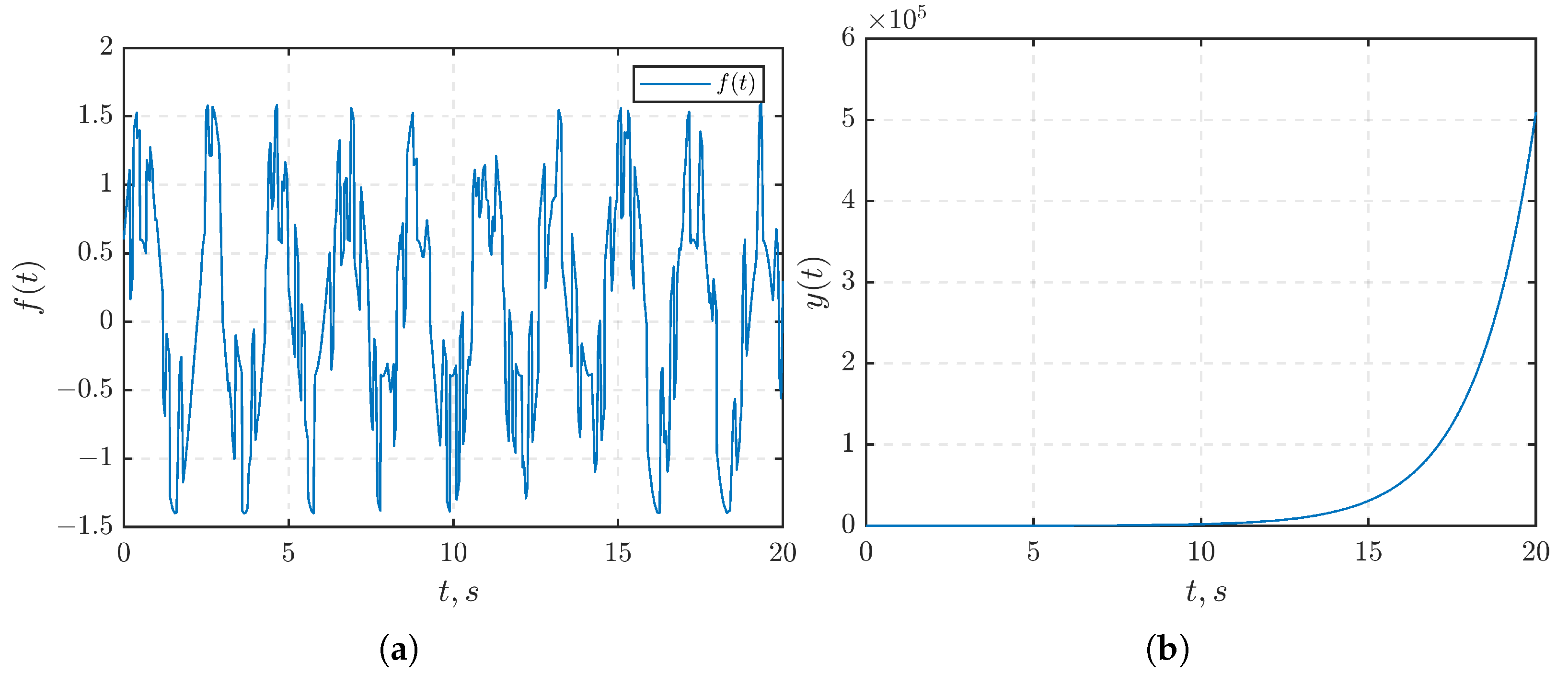
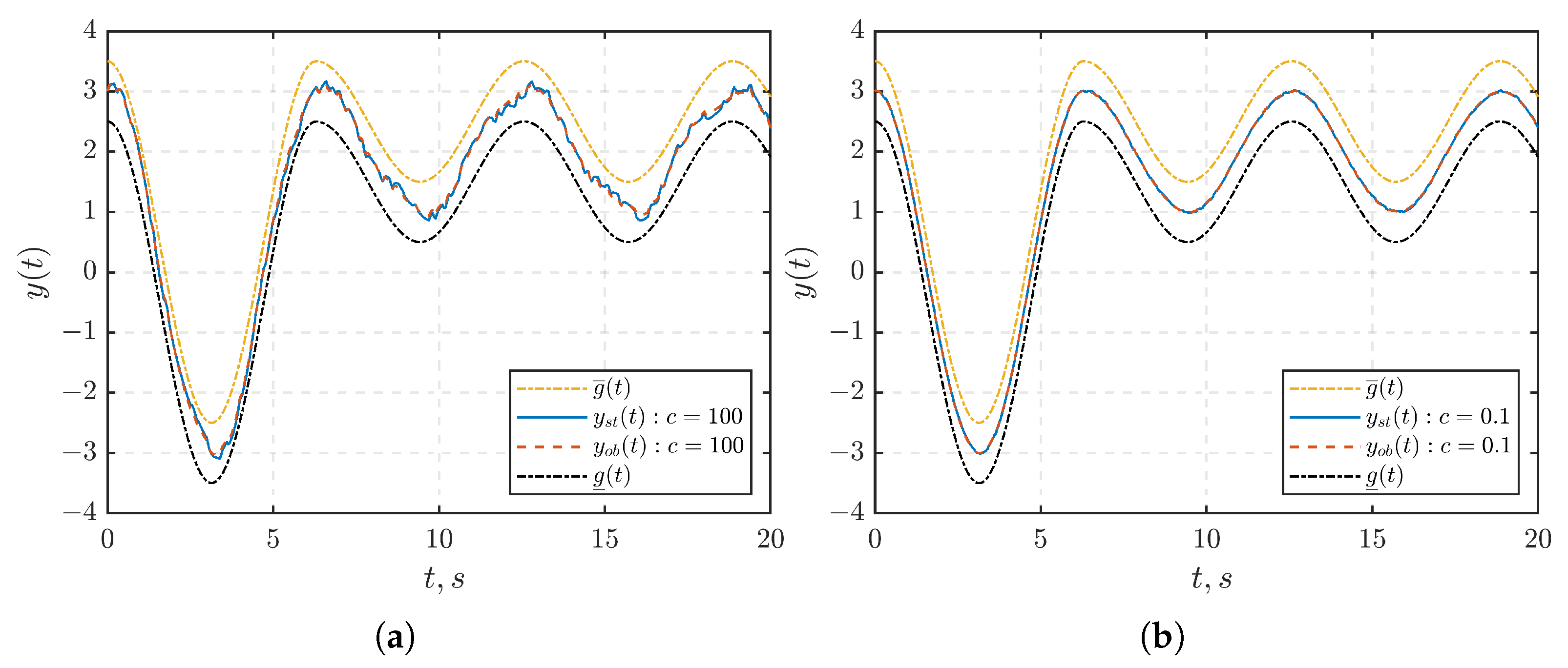
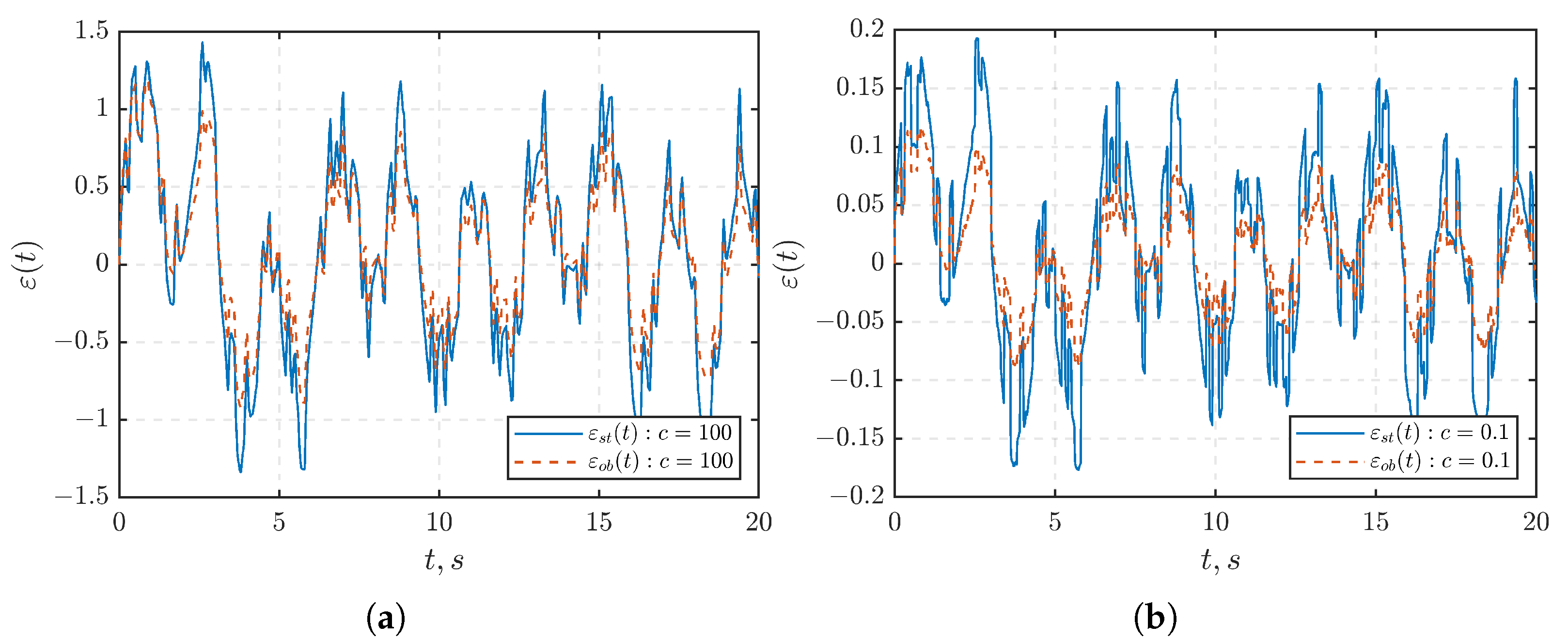
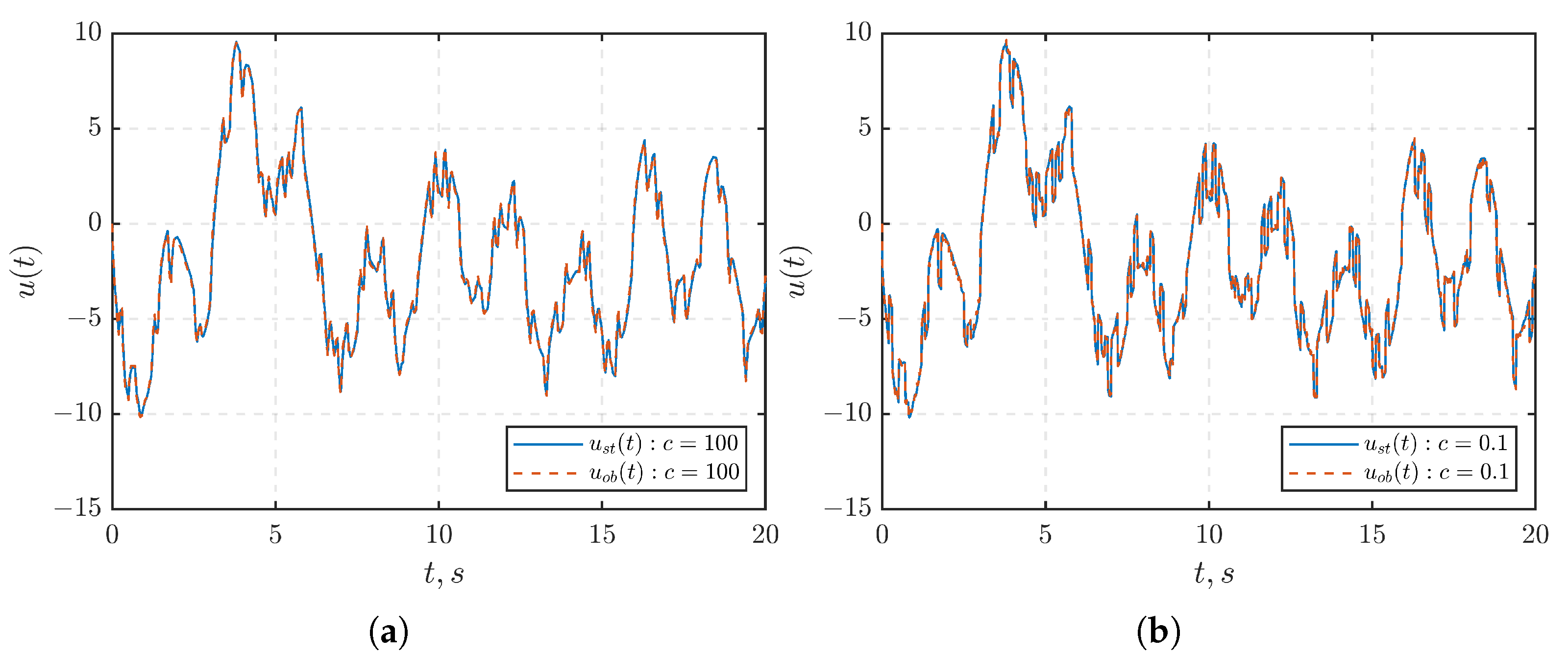
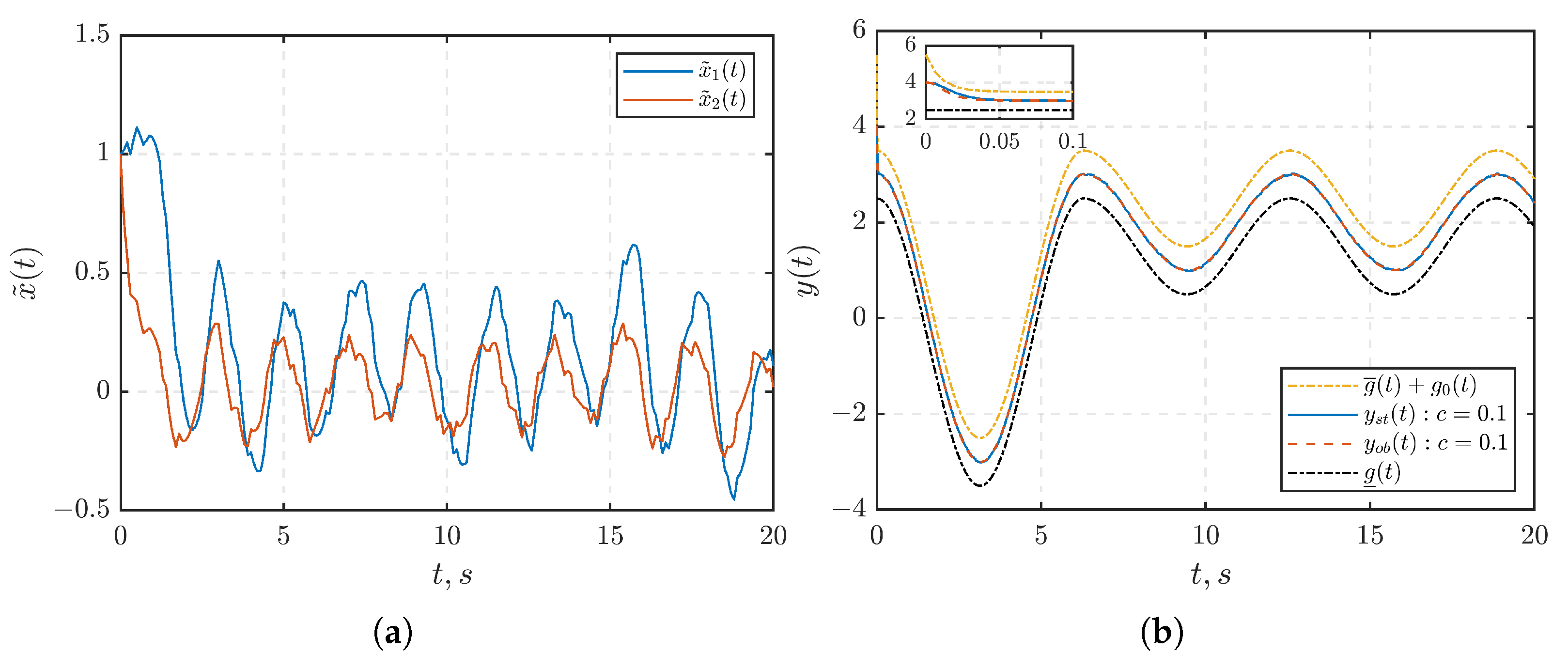
7.1. Example 1: SISO Case

Consider the system described by Equation (1) with the following parameter values

$$\begin{array}{c}A=\left[\begin{array}{cc}0& 1\\ 2& -3\end{array}\right],B=\left[\begin{array}{c}0\\ 1\end{array}\right],D=\left[\begin{array}{c}1\\ 1\end{array}\right],L=\left[\begin{array}{cc}2& 1\end{array}\right],\\ f\left(t\right)=0.1+sin\left(3t\right)+0.5sat\left\{d\left(t\right)\right\},x\left(0\right)={\left[11\right]}^T,\end{array}$$

where $sat\{·\}$ represents the saturation function and $d\left(t\right)$ is the signal modeled in Matlab/Simulink using the “Band-Limited White Noise” block with a noise power and a sampling time of 0.1. This results in $\overline{f}=1.6$. The graphic of the disturbance $f\left(t\right)$ is depicted in Figure 1a.

Figure 1. (a) The disturbance $f\left(t\right)$. (b) The open-loop step response $y\left(t\right)$.

In this example, the non-Hurwitz property of the matrix A in system (1) indicates system instability. The step response of the open-loop system (Figure 1b) shows that the output $y\left(t\right)$ goes to infinity as t increases.

To design a closed-loop system, we select the function $\epsilon \left(t\right)$ as follows

$$\epsilon \left(t\right)=ln\left(\frac{y\left(t\right)-\underline{g}\left(t\right)}{\overline{g}\left(t\right)-y\left(t\right)}\right).$$

(35)

It is evident that this function satisfies conditions (a)–(d) of transformation (3). The inverse function ${\mathrm{\Phi }}^{-1}(\epsilon ,t)$ is given by

$${\mathrm{\Phi }}^{-1}(\epsilon ,t)=\frac{\overline{g}\left(t\right)e^{\epsilon }+\underline{g}\left(t\right)}{e^{\epsilon }+1}.$$

For all $\epsilon \in \mathbb{R}$ and $t\ge 0$, it holds that

$$\frac{\partial {\mathrm{\Phi }}^{-1}(\epsilon ,t)}{\partial \epsilon }=\frac{e^{\epsilon }(\overline{g}\left(t\right)-\underline{g}\left(t\right))}{{(e^{\epsilon }+1)}^2}>0,$$

and

$$\left|\frac{\partial {\mathrm{\Phi }}^{-1}(\epsilon ,t)}{\partial t}\right|=\left|\frac{\dot{\overline{g}}\left(t\right)e^{\epsilon }+\dot{\underline{g}}\left(t\right)}{e^{\epsilon }+1}\right|\le max\{\underset{t\ge 0}{sup}|\dot{\overline{g}}\left(t\right)|,\underset{t\ge 0}{sup}|\dot{\underline{g}}\left(t\right)|\}=\gamma .$$

The parameters of the restriction functions $\underline{g}\left(t\right)$ and $\overline{g}\left(t\right)$ of the set $\mathcal{Y}$ are given as follows

$$\begin{array}{c}\overline{g}\left(t\right)=\left\{\begin{array}{cc}-3cos\left(t\right)+0.2,\hfill & t<2\pi ,\hfill \\ cos\left(t\right)+2.2,\hfill & t\ge 2\pi ,\hfill \end{array}\right.\hfill \\ \underline{g}\left(t\right)=\left\{\begin{array}{cc}3cos\left(t\right)-0.2,\hfill & t<2\pi ,\hfill \\ cos\left(t\right)+1.8,\hfill & \hfill t\ge 2\pi .\hfill \end{array}\right.\hfill \end{array}$$

For the control law based on the state feedback method (10), it is defined as

$$u\left(t\right)=-{\left(CB\right)}^{-1}\left[Kln\left(\frac{y\left(t\right)-\underline{g}\left(t\right)}{\overline{g}\left(t\right)-y\left(t\right)}\right)+CAx\left(t\right)\right].$$

Similarly, for the observer-based feedback method (26), the control law is defined as

$$u\left(t\right)=-{\left(CB\right)}^{-1}\left[Kln\left(\frac{y\left(t\right)-\underline{g}\left(t\right)}{\overline{g}\left(t\right)-y\left(t\right)}\right)+CA\widehat{x}\left(t\right)\right].$$

By choosing the eigenvalues of the observer matrix $(A-K_{o}C)$ in (28) as $\lambda =-1$ and ${\lambda }_2=-4$, the matrix $K_o$ is determined as $K_o=col\{0.5,1\}$. Consequently, the bound of $|\tilde{x}\left(t\right)|$ can be computed as $\mu =4.34$. The values of $\gamma$ and $\kappa$ are calculated as $\gamma =3$ and $\kappa =7.8$, respectively, leading to $\Delta =17.51$. To solve the inequalities (13) for the state feedback method and (34) for the observer-based method, the YALMIP package [36] is employed with the SEDUMI solver. The resulting solutions $(K,{\tau }_1,{\tau }_2)$ for $c=100$ and $c=0.1$ are presented in Table 1.

Table 1. The solutions $(K,{\tau }_1,{\tau }_2)$ of the inequalities (13) and (34) with various values of parameter c.

c	State Feedback Method	Observer-Based Method
100	(6.31, 2.68, 4.34)	(8.35, 6.69, 2.17)
0.1	(33.18, 42.66, 0.05)	(65.73, 85.65, 0.02)

The transient responses of $y\left(t\right)$, $\epsilon \left(t\right)$ and $u\left(t\right)$ with an initial condition of $x\left(0\right)=col\{1,1\}$ are illustrated in Figure 2, Figure 3 and Figure 4, respectively. Figure 5a shows the plot illustrating the observation errors. In Figure 2, it becomes evident that the output signal $y\left(t\right)$ remains within the given set at any time. Furthermore, $y\left(t\right)$ never reaches the boundaries of the given set $\mathcal{Y}$. This observation is grounded in the choice of the function $\epsilon \left(t\right)$ in (35). Specifically, if the output signal $y\left(t\right)$ reaches the boundaries $\underline{g}\left(t\right)$ or $\overline{g}\left(t\right)$ of the set $\mathcal{Y}$, then the corresponding signal $\epsilon \left(t\right)$ would go to infinity. This divergent behavior contradicts the boundedness of $\epsilon \left(t\right)$ as obtained in Figure 3.

Figure 2. The transient of output $y\left(t\right)$ in the closed-loop system under: (a) $c=100$. (b) $c=0.1$. The yellow and black dashed lines represent the performance functions $\overline{g}\left(t\right)$ and $\underline{g}\left(t\right)$. The solid blue line represents the output $y_{st}\left(t\right)$ when the state feedback controller (10) is applied, and the red dashed line represents the output $y_{ob}\left(t\right)$ when the observed-based controller (26) is applied.

Figure 3. The graphics of the auxiliary variable $\epsilon \left(t\right)$ under: (a) $c=100$. (b) $c=0.1$. The solid blue line represents the output $\epsilon \left(t\right)$ when the state feedback controller (10) is applied, and the red dashed line represents the control signal $\epsilon \left(t\right)$ when the observed-based controller (26) is applied.

Figure 4. The control signal $u\left(t\right)$ under: (a) $c=100$. (b) $c=0.1$. The solid blue line represents the control signal $u_{st}\left(t\right)$ when the state feedback controller (10) is applied, and the red dashed line represents the control signal $u_{ob}\left(t\right)$ when the observed-based controller (26) is applied.

Figure 5. (a) The observation errors $\tilde{x}\left(t\right)$. (b) The transient of output $y\left(t\right)$ in the closed-loop system under $c=0.1$ for $x\left(0\right)=col\{\frac{5}{3},\frac{2}{3}\}$.

Furthermore, as depicted in Figure 3, the signal $\epsilon \left(t\right)$ is stabilized within predefined ball regions. Specifically, at $c=100$ (Figure 3a), $\epsilon \left(t\right)$ is stabilized within a ball with a radius $r<14.14$ (approximately $r\approx 1.5$), whereas at $c=0.1$ (Figure 3b), it is stabilized within a ball with a radius $r<0.44$ (approximately $r\approx 0.2$). Upon comparing Figure 2a,b, as well as Figure 3a,b, it is important to highlight that decreasing the value of the parameter c leads to enhanced suppression of disturbance effects.

In Figure 4, the oscillations observed in the control signal can be attributed to the influence of the disturbance $f\left(t\right)$ within the system (depicted in Figure 1a). Furthermore, as mentioned in Remark 3, owing to the presence of $f\left(t\right)$, the observation errors illustrated in Figure 5a do not converge to zero. Nevertheless, the observer-based control method effectively maintains the output signal within the given set. As a result, both proposed control methods demonstrate a high level of performance in stabilizing the output of the system (1).

Remark 4. 

In the preceding example, we have assumed that the initial value of the output signal belongs to a given set. However, if the initial value of the output signal falls outside this given set, the proposed method becomes inapplicable. This limitation arises from the requirement established in transformation (3), demanding that the output signal be constrained within the predefined set. To address this limitation, we introduce an additional expedient: an exponentially decaying function with rapid decay, to augment the performance functions. By incorporating this modification, the newly defined bounds encompass the initial conditions as well.

Figure 5b illustrates the transient response of $y\left(t\right)$ for the initial condition $x\left(0\right)=col\{\frac{5}{3},\frac{2}{3}\}$, where $y\left(0\right)=4$, a value that lies outside the original set $\mathcal{Y}$. To rectify this, we introduce a term $g_0\left(t\right)=2e^{-100t}$ into the function $\overline{g}\left(t\right)$. This modification ensures that the initial condition $y\left(0\right)$ is bounded from above by the updated performance function $\overline{g}\left(t\right)+g_0\left(t\right)$.

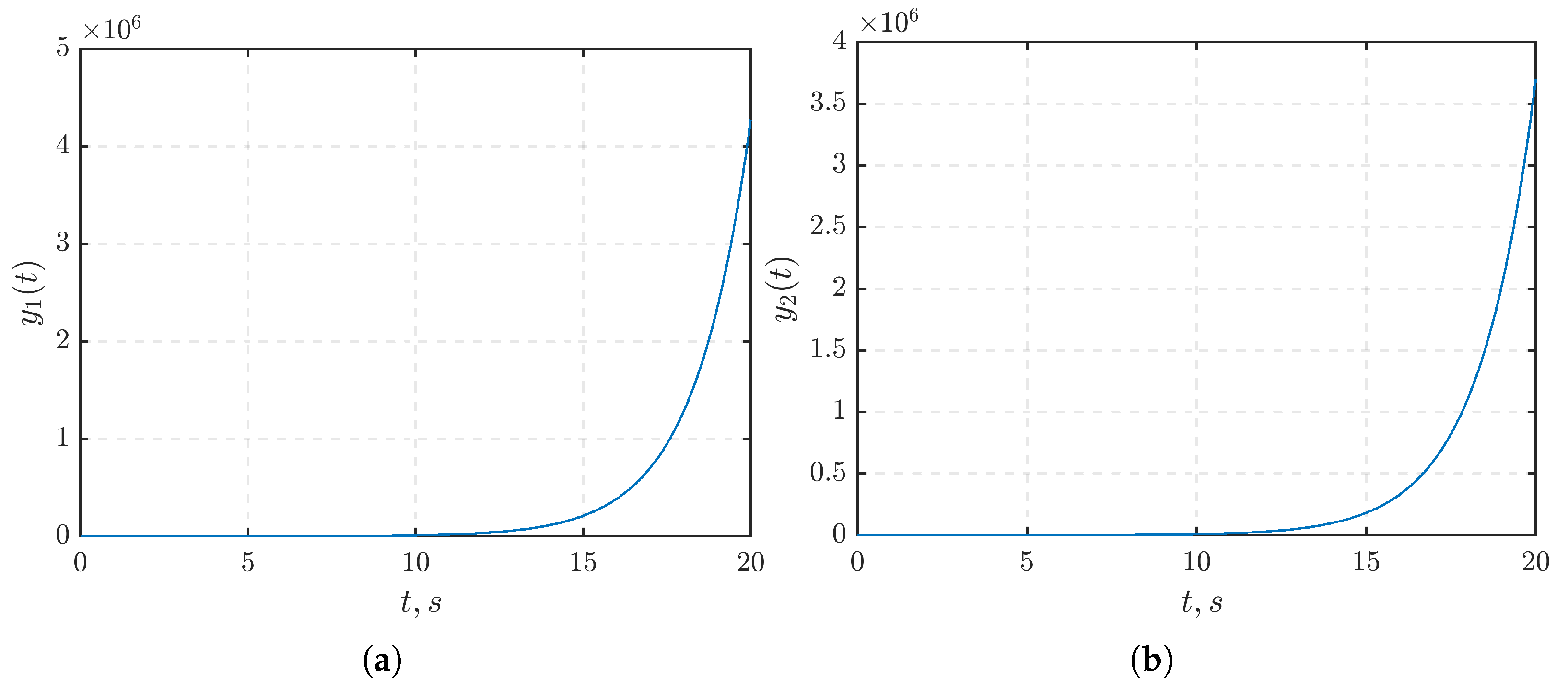
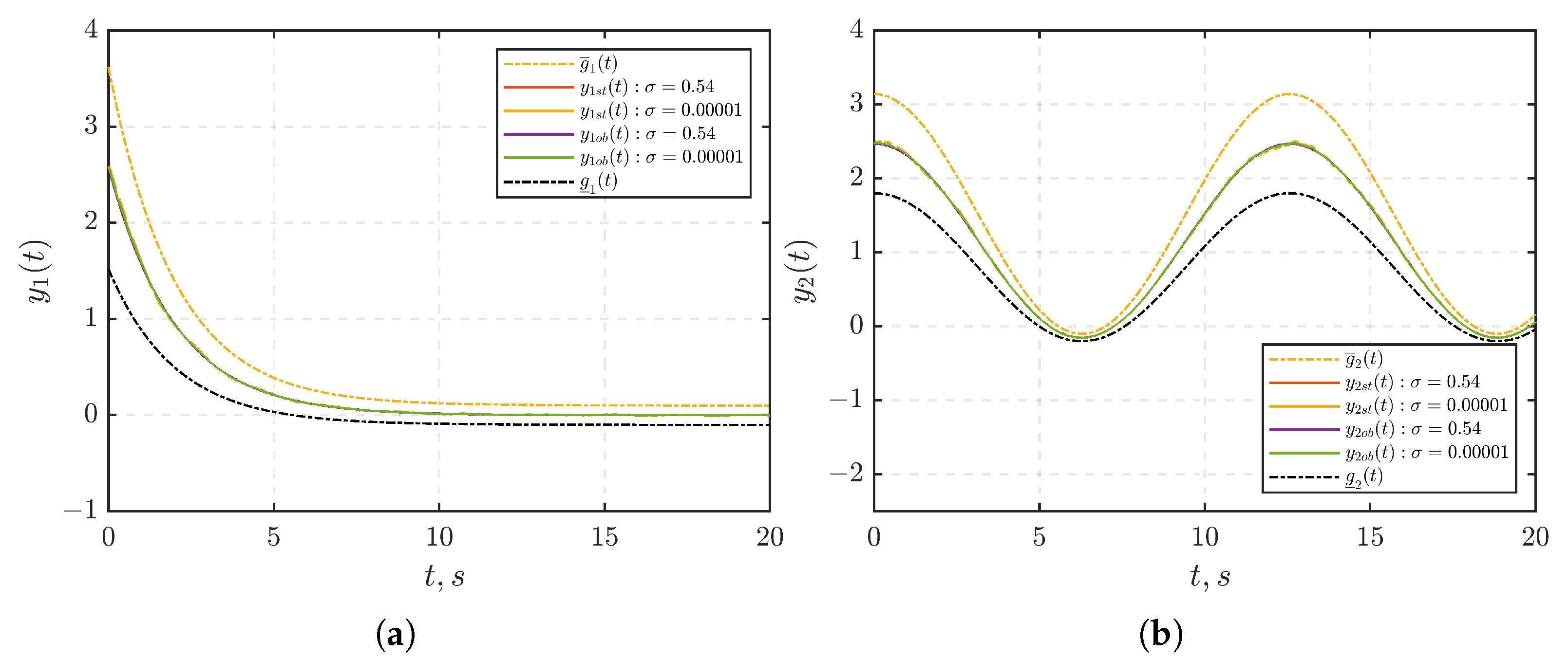
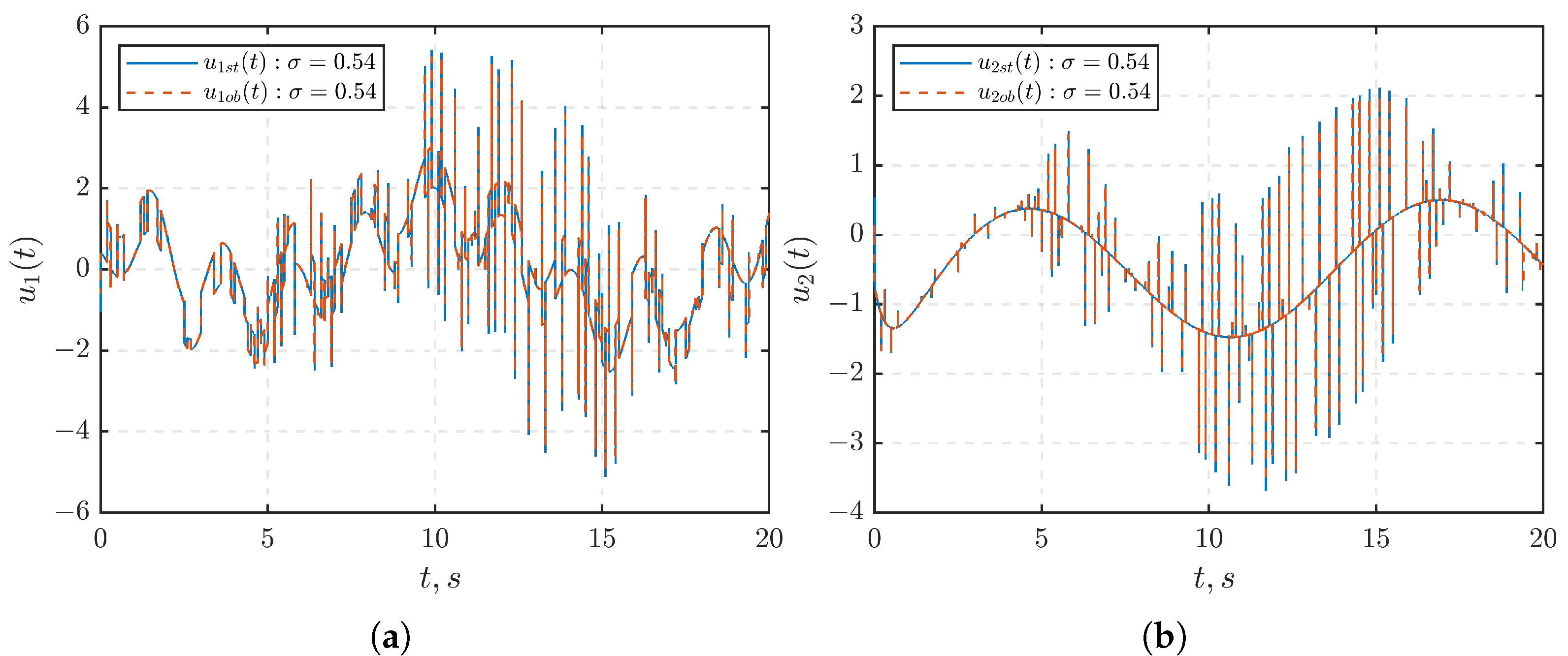
7.2. Example 2: MIMO Case

Let us demonstrate the performance of control for a system (1) with two inputs and two outputs with the following parameters

$$\begin{array}{c}A=\left[\begin{array}{ccc}0& 1& 0\\ 0& 0& 1\\ 0.1& 2& -3\end{array}\right],B=\left[\begin{array}{cc}1& 2\\ 1& 1\\ 1& 3\end{array}\right],D=\left[\begin{array}{c}1\\ 1\\ 1\end{array}\right],L=\left[\begin{array}{ccc}2& 1& 1\\ 1& 2& 1\end{array}\right],\end{array}$$

$f\left(t\right)$ is defined as shown in Section 7.1. The given system is unstable since the matrix A is non-Hurwitz. Figure 6 illustrates the step response of the open-loop system, demonstrating that the output signals $y_1\left(t\right)$ (Figure 6a) and $y_2\left(t\right)$ (Figure 6b) go to infinity as time increases.

Figure 6. The open-loop step response: (a) $y_1\left(t\right)$. (b) $y_2\left(t\right)$.

To design a closed-loop system, we formulate the function $\epsilon \left(t\right)=col\{{\epsilon }_1\left(t\right),{\epsilon }_2\left(t\right)\}$ with ${\epsilon }_i\left(t\right)$ as defined in (35)

$${\epsilon }_i\left(t\right)=ln\left(\frac{y_i\left(t\right)-{\underline{g}}_i\left(t\right)}{{\overline{g}}_i\left(t\right)-y_i\left(t\right)}\right).$$

Then, we derive the inverse functions ${\mathrm{\Phi }}_i^{-1}({\epsilon }_i,t)$ as follows:

$${\mathrm{\Phi }}_i^{-1}(\epsilon ,t)=\frac{{\overline{g}}_i\left(t\right)e^{{\epsilon }_i}+{\underline{g}}_i\left(t\right)}{e^{{\epsilon }_i}+1}.$$

For all ${\epsilon }_i\in \mathbb{R}$ and $t\ge 0$, the following results are obtained

$$\frac{\partial {\mathrm{\Phi }}_i^{-1}({\epsilon }_i,t)}{\partial {\epsilon }_i}=\frac{e^{{\epsilon }_i}({\overline{g}}_i\left(t\right)-{\underline{g}}_i\left(t\right))}{{(e^{{\epsilon }_i}+1)}^2}>0.$$

and

$$\left|\frac{\partial {\mathrm{\Phi }}_i^{-1}({\epsilon }_i,t)}{\partial t}\right|=\left|\frac{\dot{{\overline{g}}_i}\left(t\right)e^{{\epsilon }_i}+\dot{{\underline{g}}_i}\left(t\right)}{e^{{\epsilon }_i}+1}\right|\le max\{\underset{t\ge 0}{sup}|\dot{{\overline{g}}_i}\left(t\right)|,\underset{t\ge 0}{sup}|\dot{{\underline{g}}_i}\left(t\right)|\}={\gamma }_i.$$

Consequently, the matrix $\frac{\partial {\mathrm{\Phi }}^{-1}(\epsilon ,t)}{\partial \epsilon }=diag\left\{\frac{{\overline{g}}_i\left(t\right)e^{{\epsilon }_i}+{\underline{g}}_i\left(t\right)}{e^{{\epsilon }_i}+1}\right\},i=1,2$ is positive definite. Moreover, based on the last inequality, the upper bound of the function $\frac{\partial {\mathrm{\Phi }}^{-1}(\epsilon ,t)}{\partial t}$ can be estimated as $\gamma =\sqrt{2}{\gamma }_i$.

For $\epsilon \notin \mathrm{\Omega }$ we have $0\prec \frac{\partial {\mathrm{\Phi }}^{-1}(\epsilon ,t)}{\partial \epsilon }⪯\overline{\sigma }I$, where

$$\overline{\sigma }=\frac{1}{4}\underset{i}{max}\left[\underset{t\ge 0}{sup}({\overline{g}}_i\left(t\right)-{\underline{g}}_i\left(t\right))\right].$$

The parameters governing the restriction functions $\underline{g}\left(t\right)$ and $\overline{g}\left(t\right)$ are specified as follows:

$$\begin{array}{c}{\overline{g}}_1\left(t\right)=3.52e^{-0.5t}+0.1,\hfill \\ {\underline{g}}_1\left(t\right)=1.62e^{-0.5t}-0.1,\hfill \\ {\overline{g}}_2\left(t\right)=1.62cos\left(0.5t\right)+1.52,\hfill \\ {\underline{g}}_2\left(t\right)=cos\left(0.5t\right)+0.8.\hfill \end{array}$$

Then, the value of $\overline{\sigma }$ is calculated as $0.54$. By selecting the eigenvalues of the observer matrix $(A-K_{o}C)$ to be ${\lambda }_1=-1,{\lambda }_2=-4,{\lambda }_3=-5$, we determine that $K_o=\left[\begin{array}{cc}1.05& -0.62\\ -2.33& 3.46\\ -0.31& 1.23\end{array}\right]$ and $\Delta =34.50$. Utilizing the YALMIP package along with the SEDUMI solver for $\beta =0.00001,\alpha =0.01$, we find solutions $(K,{\tau }_1,{\tau }_2)$ that satisfy the inequalities (12) and (33) at a specific value $\sigma \in (0,0.54]$ for $c=0.1$. The detailed outcome is presented in Table 2.

Table 2. The solutions $(K,{\tau }_1,{\tau }_2)$ of the inequalities (12) and (33) with $c=0.1$.

$\mathit{\sigma }$	State Feedback Method	Observer-Based Method
0.00001	($diag\{3535.2,3535.2\},\mathrm{17,431},9.21$)	($diag\{\mathrm{10,092},\mathrm{10,092}\}$, 49,458, 3.22)
0.54	($diag\{40.63,40.63\}$, 104.5, 0.053)	($diag\{121.14,121.14\}$, 307.43, 0.02)

Similar to Section 7.1, it becomes evident from Figure 7 that the control laws (10) and (26) ensure the adherence of the output signals $y_1\left(t\right)$ (Figure 7a) and $y_2\left(t\right)$ (Figure 7b) of the MIMO system (1) to the prescribed sets across all times for both cases of choosing $\sigma =0.00001$ or $\sigma =0.54$. At the parameter value $c=0.1$, the external disturbance $f\left(t\right)$ is effectively suppressed. The behavior of the control signals $u_1\left(t\right)$ and $u_2\left(t\right)$ for $\sigma =0.54$ is illustrated in Figure 8a and Figure 8b, respectively. Figure 9 further illustrates the observation errors. As demonstrated in Section 7.1, achieving convergence to zero in observation errors during the design of the state observer is not necessary.

Figure 7. The transients of outputs $y_1\left(t\right)$, $y_2\left(t\right)$ in the closed-loop system under $c=0.1$ with $\sigma =0.00001$ and $\sigma =0.54$: (a) $y_1\left(t\right)$. (b) $y_2\left(t\right)$. The yellow and black dashed lines represent the performance functions $\overline{g}\left(t\right)$ and $\underline{g}\left(t\right)$. The red and orange solid lines represents the outputs $y_{1st}\left(t\right),y_{2st}\left(t\right)$ when the state feedback controller (10) is applied, and the the purple and green solid lines represents the output $y_{1ob}\left(t\right),y_{2ob}\left(t\right)$ when the observed-based controller (26) is applied.

Figure 8. The control signals $u_1\left(t\right)$ and $u_2\left(t\right)$ for $\sigma =0.54$: (a) $u_1\left(t\right)$. (b) $u_2\left(t\right)$. The solid blue line represents the control signal $u_{st}\left(t\right)$ when the state feedback controller (10) is applied, and the red dashed line represents the control signal $u_{ob}\left(t\right)$ when the observed-based controller (26) is applied.

Figure 9. The observation errors $\tilde{x}\left(t\right)$.

8. Conclusions

This paper proposed a general procedure for designing nonlinear control laws for linear systems with a guarantee of finding output signals in given sets based on the transformation of coordinates [25]. The selection function $\epsilon \left(t\right)$ in a diagonal form and using S-procedure Lemma enabled us to analyze the ISS stability of the closed-loop MIMO system consisting of a nonstationary matrix ${\left(\frac{\partial {\mathrm{\Phi }}^{-1}(\epsilon ,t)}{\partial \epsilon }\right)}^{-1}$. In this paper, two control laws were proposed depending on the measurability of the state vector, one based on state feedback and the other on observer feedback. Furthermore, the parameters for the control laws were computed utilizing LMIs, extending the applicability of the method [25] in practice. These control laws guaranteed the boundedness of the auxiliary variable $\epsilon \left(t\right)$, leading to the maintenance of the output variable $y\left(t\right)$ within the given set. By reducing the radius of the attractive set of $\epsilon \left(t\right)$ via parameter c, we reduced the effect of disturbances on the output $y\left(t\right)$. Moreover, when designing the observer for the system (1) with unknown disturbances, it is not required to ensure the convergence of observation errors to zero. Instead, the observer should be designed to guarantee the boundedness of the estimation error. As the simulation results showed, both proposed control laws demonstrated a high-performance level in stabilizing the output of the system (1) within the given set.

References

- Boldea, I. Control of Electric Generators: A Review. IECON Proc. Industrial Electron. Conf. 2003, 1, 972–980. [Google Scholar] [CrossRef]
- Furtat, I.; Nekhoroshikh, A.; Gushchin, P. Synchronization of multi-machine power systems under disturbances and measurement errors. Int. J. Adapt. Control. Signal Process. 2022, 36, 1272–1284. [Google Scholar] [CrossRef]
- Pavlov, G.; Merkurev, G. Energy Systems Automation; Papirus Publisher: St. Petersburg, Russia, 2001. (In Russian) [Google Scholar]
- Kundur, P. Power System Stability and Control; McGraw-Hill Education: New York, NY, USA, 1994; p. 1176. [Google Scholar]
- Landera, Y.G.; Zevallos, O.C.; Neves, F.A.S.; Neto, R.C.; Prada, R.B. Control of PV Systems for Multimachine Power System Stability Improvement. IEEE Access 2022, 10, 45061–45072. [Google Scholar] [CrossRef]
- Feydi, A.; Elloumi, S.; Braiek, N.B. Robustness of Decentralized Optimal Control Strategy Applied On Two Interconnected Generators System With Uncertainties. In Proceedings of the 2023 IEEE International Conference on Advanced Systems and Emergent Technologies, Hammamet, Tunisia, 29 April–1 May 2023; pp. 1–6. [Google Scholar] [CrossRef]
- Tan, H.; Cong, L. Modeling and Control Design for Distillation Columns Based on the Equilibrium Theory. Processes 2023, 11, 607. [Google Scholar] [CrossRef]
- Verevkin, A.; Kiriushin, O. Control of the formation pressure system using finite-state-machine models. Oil Gas Territ. 2008, 10, 14–19. (In Russian) [Google Scholar]
- Bouyahiaoui, C.; Grigoriev, L.I.; Laaouad, F.; Khelassi, A. Optimal fuzzy control to reduce energy consumption in distillation columns. Autom. Remote Control 2005, 66, 200–208. [Google Scholar] [CrossRef]
- Sunori, S.K.; Joshi, K.A.; Mittal, A.; Nainwal, D.; Khan, F.; Juneja, P. Improvement in Controller Performance for Distillation Column Using IMC Technique. In Proceedings of the 2023 International Conference for Advancement in Technology (ICONAT), Goa, India, 24–26 January 2023; pp. 1–5. [Google Scholar] [CrossRef]
- Ogata, K. Modern Control Engineering; Prentice Hall: Upper Saddle River, NJ, USA, 2010; Volume 5. [Google Scholar]
- Lewis, F.L.; Vrabie, D.; Syrmos, V.L. Optimal Control; John Wiley & Sons: Hoboken, NJ, USA, 2012. [Google Scholar]
- Filabadi, M.M.; Hashemi, E. Distributed Robust Control Framework for Adaptive Cruise Control Systems. In Proceedings of the 2023 American Control Conference (ACC), San Diego, CA, USA, 31 May–2 June 2023; pp. 3215–3220. [Google Scholar] [CrossRef]
- Wang, T.; Sun, Z.; Ke, Y.; Li, C.; Hu, J. Two-Step Adaptive Control for Planar Type Docking of Autonomous Underwater Vehicle. Mathematics 2023, 11, 3467. [Google Scholar] [CrossRef]
- Hassan, F.; Zolotas, A.; Halikias, G. New Insights on Robust Control of Tilting Trains with Combined Uncertainty and Performance Constraints. Mathematics 2023, 11, 3057. [Google Scholar] [CrossRef]
- Ioannou, P.A.; Sun, J. Robust Adaptive Control; PTR Prentice-Hall: Upper Saddle River, NJ, USA, 1996; Volume 1. [Google Scholar]
- Krstic, M.; Kokotovic, P.V.; Kanellakopoulos, I. Nonlinear and Adaptive Control Design; John Wiley & Sons, Inc.: Hoboken, NJ, USA, 1995. [Google Scholar]
- Narendra, K.S.; Annaswamy, A.M. Stable Adaptive Systems; Courier Corporation: Chelmsford, MA, USA, 2012. [Google Scholar]
- Tao, G. Adaptive Control Design and Analysis; John Wiley & Sons: Hoboken, NJ, USA, 2003; Volume 37. [Google Scholar]
- Xu, J.; Lin, N.; Chi, R. Improved High-Order Model Free Adaptive Control. In Proceedings of the 2021 IEEE 10th Data Driven Control and Learning Systems Conference (DDCLS), Suzhou, China, 14–16 May 2021; pp. 704–708. [Google Scholar] [CrossRef]
- Khlebnikov, M.V.; Polyak, B.T.; Kuntsevich, V.M. Optimization of linear systems subject to bounded exogenous disturbances: The invariant ellipsoid technique. Autom. Remote Control 2011, 72, 2227–2275. [Google Scholar] [CrossRef]
- Miller, D.E.; Davison, E.J. An Adaptive Controller Which Provides an Arbitrarily Good Transient and Steady-State Response. IEEE Trans. Autom. Control 1991, 36, 68–81. [Google Scholar] [CrossRef]
- Bechlioulis, C.P.; Rovithakis, G.A. Robust Adaptive Control of Feedback Linearizable MIMO Nonlinear Systems With Prescribed Performance. IEEE Trans. Autom. Control 2008, 53, 2090–2099. [Google Scholar] [CrossRef]
- Furtat, I.; Gushchin, P. Control of Dynamical Systems with Given Restrictions on Output Signal with Application to Linear Systems. IFAC Pap. 2020, 53, 6384–6389. [Google Scholar] [CrossRef]
- Furtat, I.B.; Gushchin, P.A. Control of Dynamical Plants with a Guarantee for the Controlled Signal to Stay in a Given Set. Autom. Remote Control 2021, 82, 654–669. [Google Scholar] [CrossRef]
- Polyak, B.T.; Khlebnikov, M.V.; Shcherbakov, P.S. Linear Matrix Inequalities in Control Systems with Uncertainty. Autom. Remote Control 2021, 82, 1–40. [Google Scholar] [CrossRef]
- Poznyak, A.; Polyakov, A.; Azhmyakov, V. Attractive Ellipsoids in Robust Control; Springer International Publishing: Berlin/Heidelberg, Germany, 2014. [Google Scholar] [CrossRef]
- Boyd, S.; El Ghaoui, L.; Feron, E.; Balakrishnan, V. Linear Matrix Inequalities in System and Control Theory; SIAM: Philadelphia, PA, USA, 1994. [Google Scholar]
- Fradkov, A.L.; Miroshnik, I.V.; Nikiforov, V.O. Nonlinear and Adaptive Control of Complex Systems; Springer: Berlin/Heidelberg, Germany, 1999. [Google Scholar] [CrossRef]
- Isidori, A. Nonlinear Control Systems II; Springer: Berlin/Heidelberg, Germany, 2013. [Google Scholar]
- Khalil, H.K. Nonlinear Control; Pearson: New York, NY, USA, 2015; Volume 406. [Google Scholar]
- Sturm, J.F. Using SeDuMi 1.02, a Matlab toolbox for optimization over symmetric cones. Optim. Methods Softw. 1999, 11, 625–653. [Google Scholar] [CrossRef]
- Toh, K.C.; Todd, M.J.; Toh, K.C.; Todd, M.J.; Tütüncü, R.H.; TOHal, K.C.; Tutuncu, R.H. SDPT3-a MATLAB software package for semidefinite programming, version 1.3. Optirniration Methods Softw. 1999, 11, 545–581. [Google Scholar] [CrossRef]
- Borchers, B. CSDP, A C library for semidefinite programming. Optim. Methods Softw. 1999, 11, 613–623. [Google Scholar] [CrossRef]
- Luenberger, D. An introduction to observers. IEEE Trans. Autom. Control 1971, 16, 596–602. [Google Scholar] [CrossRef]
- Löfberg, J. YALMIP: A toolbox for modeling and optimization in MATLAB. In Proceedings of the IEEE International Symposium on Computer-Aided Control System Design, Taipei, Taiwan, 2–4 September 2004; pp. 284–289. [Google Scholar] [CrossRef]
Disclaimer/Publisher’s Note: The statements, opinions and data contained in all publications are solely those of the individual author(s) and contributor(s) and not of MDPI and/or the editor(s). MDPI and/or the editor(s) disclaim responsibility for any injury to people or property resulting from any ideas, methods, instructions or products referred to in the content. |
© 2023 by the authors. Licensee MDPI, Basel, Switzerland. This article is an open access article distributed under the terms and conditions of the Creative Commons Attribution (CC BY) license (https://creativecommons.org/licenses/by/4.0/).