Regression Analysis of Dependent Current Status Data with Left Truncation

Abstract

Current status data are encountered in a wide range of applications, including tumorigenic experiments and demographic studies. In this case, each subject has one observation, and the only information obtained is whether the event of interest happened at the moment of observation. In addition to censoring, truncating is also very common in practice. This paper examines the regression analysis of current status data with informative censoring times, considering the presence of left truncation. In addition, we propose an inference approach based on sieve maximum likelihood estimation (SMLE). A copula-based approach is used to describe the relationship between the failure time of interest and the censoring time. The spline function is employed to approximate the unknown nonparametric function. We have established the asymptotic properties of the proposed estimator. Simulation studies suggest that the developed procedure works well in practice. We also applied the developed method to a real dataset derived from an AIDS cohort research.

1. Introduction

Current status data generally arise in demographic, tumorigenic, and epidemiological fields [1,2,3]. One significant feature of the current status data is that the failure time cannot be accurately observed. On the contrary, it is known that the failure time is less than or greater than the observation or examination time. One common feature of studies that produce such data is that participants are only observed once, perhaps due to the limitation of resources. In this manuscript, we consider the semiparametric regression analysis of current status data with left truncation and informative censoring. In addition, an SMLE method is proposed.

Several methods have been developed to study the current status data. For example, under the proportional hazards (PH) model, ref. [1] considered the efficiency problem and established asymptotic properties of maximum likelihood estimators of regression parameters and baseline cumulative hazard functions. Ref. [4] studied this problem under the additive hazard model and proposed an estimation equation approach to estimate the regression coefficient. Ref. [5] discussed the regression analysis problem under the proportional odds model.

Note that all the literature above assume that the failure time is independent of the examination or observation time. When the two are not independent, the data obtained are generally referred to as current status data with informative observation times or dependent current status data. Currently, some literature studies have discussed the regression analysis of current status data under the assumption of informative censoring. For example, ref. [2] discusses the regression analysis of the current status with informative examination times under the additive hazards regression model. Ref. [6] developed a class of semiparametric transformation models for dependent current status data. The above literature studies introduced frailty to depict the correlation between failure time and examination time. It is well-known that this method needs to assume the specific distribution of the latent variable, which makes the application of this method limited. An alternative way to describe the correlation between the failure time and the examination time is by introducing the copula function. For example, ref. [7] employed this method and discussed the regression analysis of current status data under the PH model. Note that the copula method has been applied in many types of dependent data analyses [8,9,10].

In addition to censoring, truncation is another statistical phenomenon that arises in various fields, including survival analysis, astronomy, epidemiology, and economics [11,12,13,14,15]. Subjects whose failure times were truncated were unable to provide any information to researchers. When only the data of individuals whose event times exceeded a certain random time (i.e., left truncation time) are recorded, left truncation will occur. Under left truncation, individuals with smaller event times are less likely to be observed, leading to bias in the research sample toward larger event times. Currently, some literature studies have developed regression analyses of current status data with left truncation [16,17]. In the following, we will discuss the regression analyses of current status data with left truncation and informative censoring.

The remainder of the article is structured as follows: We introduce the models and assumptions in Section 2. In Section 3, we introduce the SMLE method, including the estimation procedure and asymptotic properties. In Section 4, we conduct simulation studies to evaluate the practical performance of the developed approach. In Section 5, we apply the established approaches to a real dataset. Our discussions and concluding remarks are presented in Section 6.

2. Notation, Assumptions, and Models

Suppose that a failure time study consists of n independent subjects. For subject i, let $T_i$ represent the failure time and $Z_i$ be the p-dimensional vector of the covariate associated with the subject. As mentioned above, truncation is also very common in practice. For this, assume that, for every subject, there exists a left truncation time $A_i$, such that $A_i\le T_i$. The examination time is denoted by $Y_i$. It is possible that Y is dependent on the failure time $T_i$. Define ${\delta }_i=I(T_i\le Y_i)$. The observed data can be represented as follows: $\{D_i=(A_i,{\delta }_i,Y_i,Z_i),i=1,2,...,n\}$. In other words, for the failure time $T_i$, we only have current status data with the left truncation available.

We assume that $T_i$ follows a Cox model given by

$$h\left(t\right|Z)=h_{10}\left(t\right)exp\left({\alpha }^{\prime }Z\right),$$

(1)

where $h\left(t\right|Z)$ is the hazard function of $T_i$ given $Z_i$, $h_{10}\left(t\right)$ denotes an unspecified baseline hazard function, and $\alpha$ denotes a $p\times 1$ vector of regression coefficients.

In practice, the covariate may also affect the observation time $Y_i$. So, we suppose that the hazard function of $Y_i$ has the following form

$$h\left(y\right|Z)=h_{20}\left(y\right)exp\left({\eta }^{\prime }Z\right),$$

(2)

where $h_{20}\left(y\right)$ represents an unknown baseline hazard function, and $\eta$ represents the regression parameter.

To show the correlation between $T_i$ and $Y_i$, we next introduce the Copula function. Let $F(·,·)$ represent the joint distribution function of $T_i$ and $Y_i$ given $Z_i$. Thus, according to Theorem 2.3.3 in [9], there exists a copula function ${\mathbb{C}}_{\mu }(u,v)$, satisfying

$$F(t,y)={\mathbb{C}}_{\mu }(F_T\left(t\right),F_Y\left(y\right)),$$

where $F_T(·)$ and $F_Y(·)$ denote the marginal distribution function of $T_i$ and $Y_i$, respectively, $\mu$ is the association parameter representing the correlation between $T_i$ and $Y_i$. ${\mathbb{C}}_{\mu }(u,v)$ satisfies ${\mathbb{C}}_{\mu }(u,0)={\mathbb{C}}_{\mu }(0,v)=0$, ${\mathbb{C}}_{\mu }(u,1)=u$, and ${\mathbb{C}}_{\mu }(1,v)=v$. We then have the conditional distribution function of $T_i$ given $Y_i$ and $Z_i$, as follows:

$$\mathbb{P}(T⩽t|Y=y,Z)=\frac{\partial {\mathbb{C}}_{\mu }(u,v)}{\partial v}{|}_{u=F_T\left(t\right),v=F_Y\left(y\right)}=m_{\mu }(F_T\left(t\right),F_Y\left(y\right)).$$

Let $H_{10}\left(t\right)={\int }_0^t{h}_{10}\left(s\right)ds$, $H_{20}\left(y\right)={\int }_0^y{h}_{20}\left(s\right)ds$ and $\theta =(\alpha ,\eta ,H_1,H_2)$. We define $f_Y(·)$ to be the marginal density function of $Y_i$, given the covariate, so we can obtain

$$F_T\left(t\right)=1-exp\left\{-H_{10}\left(t\right)exp\left({\alpha }^{\prime }Z\right)\right\},$$

$$F_Y\left(y\right)=1-exp\left\{-H_{20}\left(y\right)exp\left({\eta }^{\prime }Z\right)\right\},$$

and

$$f_Y\left(y\right)=exp\left\{-H_{20}\left(y\right)exp\left({\eta }^{\prime }Z\right)\right\}{h}_{20}\left(y\right)exp\left({\eta }^{\prime }Z\right).$$

When $\delta =1$, we have

$$\begin{array}{cc}\hfill \mathbb{P}(\delta =1,Y|T\ge A,Y\ge A,Z)& =\frac{\mathbb{P}(A\le T\le Y,Y|Z)}{\mathbb{P}(T\ge A,Y\ge A|Z)}\hfill \\ \hfill & =\frac{f_Y\left(Y\right)\left[m_{\mu }(F_T\left(Y\right),F_Y\left(Y\right))-m_{\mu }(F_T\left(A\right),F_Y\left(Y\right))\right]}{1-F_T\left(A\right)-F_Y\left(A\right)-{\mathbb{C}}_{\mu }(F_T\left(A\right),F_Y\left(A\right))}.\hfill \end{array}$$

For $\delta =0$, we have

$$\begin{array}{cc}\hfill \mathbb{P}(\delta =0,Y|T\ge A,Y\ge A,Z)& =\frac{\mathbb{P}(T>Y,Y|Z)}{\mathbb{P}(T\ge A,Y\ge A|Z)}\hfill \\ \hfill & =\frac{f_Y\left(Y\right)\left[1-m_{\mu }(F_T\left(Y\right),F_Y\left(Y\right))\right]}{1-F_T\left(A\right)-F_Y\left(A\right)-{\mathbb{C}}_{\mu }(F_T\left(A\right),F_Y\left(A\right))}.\hfill \end{array}$$

Therefore, the likelihood function based on $(A,\delta ,Y,Z)$ is

$$\frac{f_Y\left(Y\right){\left[m_{\mu }(F_T\left(Y\right),F_Y\left(Y\right))-m_{\mu }(F_T\left(A\right),F_Y\left(Y\right))\right]}^{\delta }{\left[1-m_{\mu }(F_T\left(Y\right),F_Y\left(Y\right))\right]}^{1-\delta }}{1-F_T\left(A\right)-F_Y\left(A\right)-{\mathbb{C}}_{\mu }(F_T\left(A\right),F_Y\left(A\right))}.$$

Thus, the full likelihood function based on the i.i.d. sample $(A_i,{\delta }_i,Y_i,Z_i)$ has the following form

$$L_n\left(\theta \right)=\prod _{i=1}^n\frac{f_Y\left(Y_i\right){\left[m_{\mu }(F_T\left(Y_i\right),F_Y\left(Y_i\right))-m_{\mu }(F_T\left(A_i\right),F_Y\left(Y_i\right))\right]}^{{\delta }_i}{\left[1-m_{\mu }(F_T\left(Y_i\right),F_Y\left(Y_i\right))\right]}^{1-{\delta }_i}}{1-F_T\left(A_i\right)-F_Y\left(A_i\right)-{\mathbb{C}}_{\mu }(F_T\left(A_i\right),F_Y\left(A_i\right))}.$$

In the next part, we will consider the maximization of the above likelihood function. It should be noted that, as mentioned by [3], given a specified parametric copula family, the associated parameter $\mu$ cannot be identified without prior or additional information. Hence, in the next section, we assume that both the copula functions and the associated parameters are necessary.

3. Maximum Likelihood Estimation

Now, we discuss how to maximize the full likelihood function $L_n\left(\theta \right)$. In fact, it is difficult to directly maximize the likelihood function because this likelihood function contains not only finite-dimensional parameters but also infinite-dimensional parameter functions, $H_1(·)$ and $H_2(·)$. In order to maximize the likelihood function, we intend to approximate $H_1(·)$ and $H_2(·)$ by linear combinations of some basic functions. Specifically, we intend to use the I-spline function to accomplish this task [18]. Let ${\left\{I_d\left(t\right)\right\}}_{d=1}^{k+m_n}$ represent the I-spline base function, where k and $m_n$ are the order of the spline and the number of interior knots, respectively. Additionally, $m_n=o\left(n^{\nu }\right)$ and $0<\nu <0.5$. Then, we define

$$\begin{array}{cc}\hfill & {\mathcal{G}}_n^j=\left\{H_{jn}:H_{jn}\left(s\right)=\sum _{d=1}^{k+m_n}{\varphi }_{jd}{I}_d\left(t\right),{\varphi }_{jd}\ge 0,d=1,2,...,k+m_n,s\in [l,u]\right\}\hfill \end{array}$$

as the sieve space, $j=1,2$, and $[l,u]$ denote the range of $\left\{A_i,Y_i,i=1,2,...,n\right\}$. Thus, the functions in ${\mathcal{G}}_n^j$ are all non-negative and non-decreasing on the interval $\left[l_{,}u\right]$ [18]. Therefore, we can employ $H_{jn}(·)$ to approximate or replace $H_j(·)$ in the likelihood function, and estimate the regression parameters $\alpha$, $\eta$ and coefficients ${\varphi }_j={\left\{{\varphi }_{jd}\right\}}_{d=1}^{k+m_n}$ simultaneously by maximizing the $L_n\left(\theta \right)$ subject to ${\varphi }_{jd}\ge 0$, $j=1,2$.

One issue when using splines is how to choose k and $m_n$. An easy way to do this for a given problem is to try several different values for k and $m_n$ and compare the results. Furthermore, we can employ the Bayesian information criteria (BIC) to choose k and $m_n$, which give the smallest BIC values.

Let ${\widehat{\theta }}_n=({\widehat{\alpha }}_n,{\widehat{\eta }}_n,{\widehat{H}}_{1n}(·),{\widehat{H}}_{2n}(·))$ represent the estimator of $\theta$ described above and ${\theta }_0=({\alpha }_0,{\eta }_0,$$H_{10}(·),H_{20}(·))$ be the true value of $\theta$. To establish the asymptotic properties, we need to describe the regularity conditions first.

(C1)

The copula functions are differentiable and the partial derivatives satisfy the Lipschitz condition.

(C2)

The covariate Z has bounded support in $R^p$.

(C3)

(i) If a constant ${ϵ}_0$ and the constant vector ${\zeta }_0$ satisfy ${\zeta }_0^{T}Z=c_0$ almost surely, then ${ϵ}_0=0$ and ${\zeta }_0=0$. (ii) Assume that for any open set B in $[0,1]\times [0,1]$, ${\omega }_{\mathbb{C}}\left(B\right)>0$, where ${\omega }_{\mathbb{C}}$ represents the probability measure generated by the copula function $\mathbb{C}$.

(C4)

For $\vartheta ={({\alpha }^{\prime },{\eta }^{\prime })}^{\prime }$, suppose that the Fisher matrix $E\left(S_{\vartheta }{S}_{\vartheta }^{\prime }\right)$ is positive-definite, where $S_{\vartheta }$ is defined in Appendix A.

(C5)

Let $H_j^{\left(k\right)}(·)$ denote the kth derivative of $H_j(·)$, $j=1,2$. Assume they are Holder-continuous with exponent $\omega$. In other words, there exists a positive constant K and some $\eta \in (0,1]$, such that $|H_j^{\left(k\right)}\left(t_1\right)-H_j^{\left(k\right)}\left(t_2\right)|\le K|t_1-t_2{|}^{\omega }$ for all $t_1,t_2\in (l,u)$. In the following, let $r=k+\omega .$

According to [19,20], the aforementioned conditions are typically moderate and meet in practical situations. The following theorems provide the large sample properties of the estimators. Here, for function g, let ${\parallel g\left(X\right)\parallel }_2={(\int |g\left(X\right)|}^2{d\mathbb{P})}^{1/2}$, where $\mathbb{P}$ is the probability measure generated by X.

Theorem 1.

Assume that the regularity conditions C1–C4 are satisfied. Then,

$${\widehat{\alpha }}_n⟶0,{\widehat{\eta }}_n⟶0,$$

$$\parallel {\widehat{H}}_{1n}-H_{10}{\parallel }_2⟶0,{\parallel {\widehat{H}}_{2n}-H_{20}\parallel }_2⟶0$$

almost surely.

Theorem 2.

Assume that the regularity conditions C1–C4 are satisfied. Then

$$\parallel {\widehat{H}}_{1n}-H_{10}{\parallel }_2+{\parallel {\widehat{H}}_{2n}-H_{20}\parallel }_2=O_p(n^{-(1-\nu )/2}+n^{-r\nu }).$$

Theorem 3.

Assume that conditions C1–C5 are satisfied and $r>2$. Then, as $n⟶\infty$, we have $\sqrt{n}{({({\widehat{\alpha }}_n-{\alpha }_0)}^{\prime },{({\widehat{\eta }}_n-{\eta }_0)}^{\prime })}^{\prime }\stackrel{d}{⟶}N(0,\Sigma )$; the definition of Σ is in Appendix A.

We provide the proof of the above theorems in the appendix. In order to estimate the covariance matrix, we recommend a common and direct method based on the sieve likelihood function, i.e., using the inverse of the observed information matrix. The observed information may be poorly conditioned or high-dimensional, so this method might be computationally demanding. Nevertheless, the simulation results shown in the following section suggest that it typically performs effectively, particularly when k and $m_n$ are not very big.

4. Simulation Study

In this section, simulation studies are conducted to evaluate the performance of the developed procedure. We suppose that the $Z_i$ covariates are Bernoulli (0.5). We first generate the left truncation time $A_i$ from the exponential distribution with parameters a, where constant a is selected to provide a suitable percentage of the left truncation. We set $H_{10}\left(t\right)=t$, and $T_i$ is generated from model (1). To generate the examination time $Y_i$, we consider the following three copula models:

$${\mathbb{C}}_{\mu }(u,v)=\left\{\begin{array}{c}uv+\mu uv(1-u)(1-v),-1⩽\mu ⩽1,\hfill \\ {log}_{\mu }\left\{1-\frac{(1-{\mu }^u)(1-{\mu }^v)}{1-\mu }\right\},\mu >0,\mu \ne 1,\hfill \\ exp\left\{-{[{(-logu)}^{\mu }+{(-logv)}^{\mu }]}^{1/\mu }\right\},\mu \ge 1.\hfill \end{array}\right.$$

They are the FGM, Frank, and Gumbel models, respectively. As mentioned above, the association parameter $\mu$ here indicates the correlation between T and Y. Since the range of $\mu$ in the above three copula models are not the same, one needs a uniform measure of association between T and Y, such as Kendall’s $\tau$. For the FGM model, $\tau =2\mu /9$, and $\tau =1+4h^{-1}\left\{B_1\left(h\right)-1\right\}$ for the Frank model, $h=-log\mu$ and $B_1\left(h\right)=h^{-1}{\int }_0^{h}x{(e^x-1)}^{-1}dx$. Under the Gumbel model, the relationship is $\tau =1-1/\mu$.

Based on a fixed copula function, we set $H_{20}\left(y\right)=y$, then the examination time $Y_i$ is generated from the conditional distribution, given $T_i$. Specifically, we first generate a random number $b\sim U(0,1)$; given $T_i=t_i$ and b, we can solve the following equation for $Y_i=y_i$,

$$\mathbb{P}(Y_i⩽y_i|T=t_i,Z_i)=\frac{\partial {\mathbb{C}}_{\mu }(u,v)}{\partial u}{|}_{u=F_T\left(t_i\right),v=F_Y\left(y_i\right)}=b.$$

For the spline functions, we employ the quadratic splines with the $1/4,1/2,3/4$ quantiles of the pooled set of all $A_i$’s and $Y_i$’s as three interior knots. The results shown below are based on 1000 replications.

Table 1 and Table 2 report the simulation results under the FGM model with sample sizes $n=200$ and 400. The results show the estimated bias (bias, empirical average of the parameter estimator minus the true value), the standard error of the parameter estimator (SSE), the empirical average of the standard error estimator (SEE), and the empirical coverage percentage of the 95% confidence interval (CP). 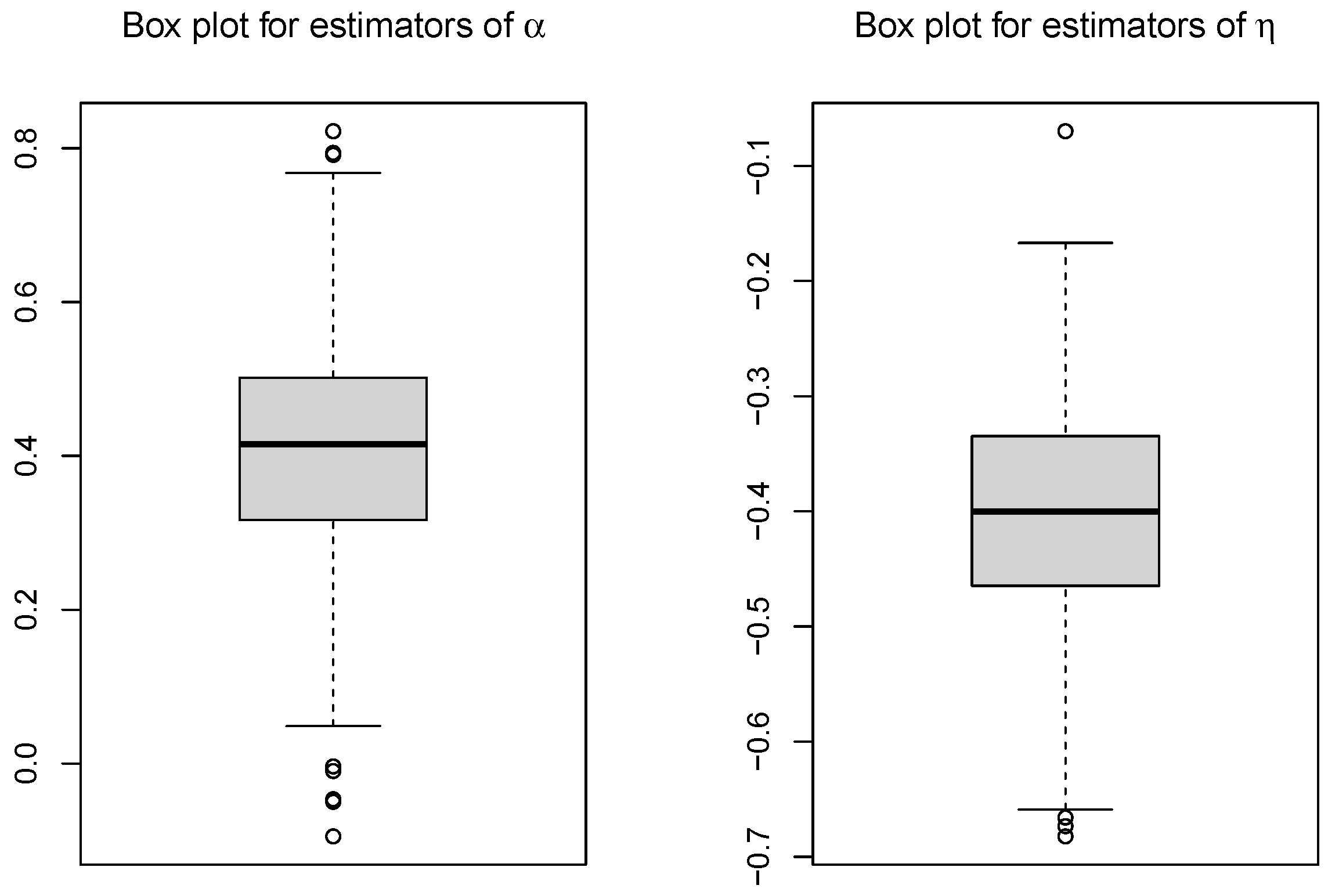Figure 1 presents the boxplots of estimators of $\alpha$ and $\eta$ with ${\alpha }_0=0.4$ and ${\eta }_0=-0.4$ under the FGM copula. It can be seen that the estimators have a slight bias, and the bias becomes smaller as n increases. The true variabilities are accurately reflected by the variance estimators, and the confidence intervals have proper coverage probabilities, i.e., the normal approximation to the distribution of the estimated regression parameters seems reasonable. The estimation results based on the Frank and Gumbel copulas are presented in Table 3, Table 4, Table 5 and Table 6; they yield comparable conclusions to those given in Table 1.

Table 1. Simulation results under the FGM model with $n=200$.

			$\widehat{\mathit{\alpha }}$				$\widehat{\mathit{\eta }}$
${\mathit{\alpha }}_0$	${\mathit{\eta }}_0$	${\mathit{\tau }}_0$	Bias	SSE	SEE	CP	Bias	SSE	SEE	CP
0	−0.4	−0.2	−0.0034	0.2322	0.2284	0.952	−0.0202	0.1605	0.1576	0.936
		−0.1	−0.0141	0.2119	0.2145	0.953	−0.0077	0.1565	0.1508	0.953
		0	−0.0135	0.2061	0.2056	0.964	-0.0087	0.1418	0.1452	0.960
		0.1	−0.0001	0.2002	0.1980	0.946	0.0032	0.1442	0.1420	0.954
		0.2	0.0045	0.1922	0.1901	0.950	0.0023	0.1359	0.1398	0.952
	0	−0.2	0.0206	0.2340	0.2281	0.952	−0.0052	0.1587	0.1550	0.940
		−0.1	−0.0108	0.2162	0.2148	0.951	0.0013	0.1485	0.1476	0.945
		0	−0.0100	0.2030	0.2034	0.952	0.0090	0.1413	0.1426	0.966
		0.1	−0.0087	0.2106	0.1944	0.912	0.0014	0.1449	0.1390	0.948
		0.2	−0.0022	0.1906	0.1864	0.951	−0.0041	0.1411	0.1361	0.943
	0.4	−0.2	0.0066	0.2612	0.2363	0.932	0.0093	0.1617	0.1580	0.946
		−0.1	0.0120	0.2282	0.2209	0.934	0.0181	0.1514	0.1505	0.966
		0	0.0158	0.2160	0.2097	0.942	0.0112	0.1498	0.1454	0.952
		0.1	0.0077	0.2044	0.2016	0.938	0.0010	0.1509	0.1421	0.934
		0.2	0.0196	0.2025	0.1919	0.937	0.0138	0.1447	0.1399	0.951
0.4	−0.4	−0.2	−0.0066	0.2274	0.2223	0.949	−0.0101	0.1664	0.1613	0.947
		−0.1	0.0219	0.2224	0.2159	0.958	−0.0113	0.1545	0.1521	0.942
		0	0.0113	0.2170	0.2109	0.949	−0.0024	0.1551	0.1453	0.935
		0.1	0.0353	0.2263	0.2060	0.936	0.0012	0.1497	0.1423	0.938
		0.2	0.0122	0.2058	0.2004	0.949	0.0020	0.1424	0.1413	0.959
	0	−0.2	0.0218	0.2315	0.2242	0.946	0.0052	0.1614	0.1581	0.938
		−0.1	0.0213	0.2299	0.2153	0.938	−0.0089	0.1553	0.1488	0.952
		0	0.0314	0.2096	0.2067	0.938	−0.0016	0.1495	0.1429	0.934
		0.1	0.0222	0.2091	0.1989	0.945	0.0002	0.1473	0.1389	0.935
		0.2	0.0366	0.1965	0.1915	0.941	0.0052	0.1331	0.1357	0.961
	0.4	−0.2	0.0250	0.2542	0.2345	0.933	0.0042	0.1682	0.1597	0.947
		−0.1	0.0373	0.2407	0.2212	0.926	0.0079	0.1504	0.1512	0.954
		0	0.0269	0.2081	0.2109	0.950	0.0074	0.1366	0.1454	0.964
		0.1	0.0010	0.2009	0.2017	0.957	0.0147	0.1417	0.1416	0.955
		0.2	0.0148	0.1941	0.1953	0.937	0.0076	0.1388	0.1388	0.949

Table 2. Simulation results under the FGM model with $n=400$.

			$\widehat{\mathit{\alpha }}$				$\widehat{\mathit{\eta }}$
${\mathit{\alpha }}_0$	${\mathit{\eta }}_0$	${\mathit{\tau }}_0$	Bias	SSE	SEE	CP	Bias	SSE	SEE	CP
0	−0.4	−0.2	0.0099	0.1643	0.1589	0.945	−0.0158	0.1191	0.1106	0.929
		−0.1	−0.0104	0.1586	0.1498	0.940	−0.0154	0.1027	0.1058	0.950
		0	−0.0020	0.1432	0.1430	0.958	−0.0047	0.1056	0.1023	0.942
		0.1	0.0074	0.1376	0.1372	0.963	0.0037	0.0979	0.1002	0.955
		0.2	0.0191	0.1444	0.1322	0.919	0.0069	0.1017	0.0985	0.937
	0	−0.2	0.0078	0.1655	0.1594	0.941	−0.0080	0.1070	0.1086	0.945
		−0.1	0.0013	0.1502	0.1493	0.943	−0.0044	0.1000	0.1037	0.957
		0	0.0001	0.1444	0.1416	0.944	−0.0042	0.0956	0.1004	0.960
		0.1	0.0016	0.1399	0.1349	0.940	−0.0011	0.0986	0.0980	0.952
		0.2	0.0001	0.1329	0.1290	0.955	0.0084	0.0964	0.0961	0.951
	0.4	−0.2	0.0118	0.1655	0.1637	0.956	−0.0010	0.1100	0.1104	0.952
		−0.1	0.0163	0.1643	0.1537	0.934	0.0034	0.1093	0.1057	0.942
		0	0.0012	0.1488	0.1460	0.942	0.0060	0.1057	0.1023	0.944
		0.1	0.0119	0.1408	0.1401	0.937	0.0100	0.0989	0.1003	0.955
		0.2	0.0055	0.1387	0.1341	0.933	−0.0023	0.0940	0.0986	0.957
0.4	−0.4	−0.2	0.0019	0.1632	0.1551	0.930	−0.0139	0.1175	0.1129	0.938
		−0.1	−0.0144	0.1536	0.1494	0.949	−0.0066	0.1072	0.1068	0.953
		0	0.0118	0.1526	0.1449	0.942	−0.0018	0.1029	0.1023	0.958
		0.1	0.0133	0.1470	0.1411	0.941	−0.0017	0.1044	0.1007	0.937
		0.2	0.0027	0.1436	0.1376	0.931	0.0047	0.0957	0.0998	0.957
	0	−0.2	0.0298	0.1574	0.1565	0.949	−0.0142	0.1177	0.1102	0.927
		−0.1	0.0131	0.1446	0.1491	0.963	−0.0063	0.1091	0.1047	0.935
		0	0.0127	0.1491	0.1434	0.944	0.0052	0.0954	0.1006	0.966
		0.1	0.0125	0.1379	0.1377	0.958	0.0047	0.1032	0.0981	0.932
		0.2	0.0047	0.1414	0.1330	0.950	−0.0046	0.1015	0.0962	0.934
	0.4	−0.2	0.0263	0.1687	0.1638	0.938	−0.0001	0.1132	0.1119	0.948
		−0.1	0.0205	0.1602	0.1542	0.928	0.0062	0.1068	0.1064	0.952
		0	0.0131	0.1538	0.1467	0.950	0.0106	0.1032	0.1026	0.938
		0.1	0.0014	0.1458	0.1407	0.937	0.0027	0.1052	0.0999	0.943
		0.2	0.0001	0.1286	0.1351	0.955	0.0088	0.0937	0.0978	0.965

Figure 1. Boxplots for the estimators of $\alpha$ and $\eta$ with ${\alpha }_0=0.4$ and ${\eta }_0=-0.4$ under the FGM copula.

Table 3. Simulation results under the Frank model with $n=200$.

			$\widehat{\mathit{\alpha }}$				$\widehat{\mathit{\eta }}$
${\mathit{\alpha }}_0$	${\mathit{\eta }}_0$	${\mathit{\tau }}_0$	Bias	SSE	SEE	CP	Bias	SSE	SEE	CP
0	−0.4	−0.25	−0.0036	0.2313	0.2262	0.945	−0.0034	0.1642	0.1618	0.941
		−0.1	−0.0109	0.2287	0.2142	0.948	−0.0202	0.1545	0.1510	0.942
		−0.05	−0.0136	0.2098	0.2093	0.942	−0.0155	0.1560	0.1475	0.942
		0.05	0.0053	0.2102	0.2014	0.934	−0.0078	0.1456	0.1433	0.938
		0.1	0.0080	0.1931	0.1968	0.951	−0.0173	0.1482	0.1421	0.941
		0.25	0.0028	0.1940	0.1866	0.935	−0.0075	0.1355	0.1397	0.961
	0	−0.25	0.0104	0.2427	0.2260	0.931	0.0051	0.1640	0.1587	0.943
		−0.1	0.0084	0.2261	0.2131	0.936	0.0017	0.1479	0.1476	0.958
		−0.05	0.0008	0.2231	0.2083	0.924	−0.0093	0.1414	0.1448	0.954
		0.05	−0.0070	0.1939	0.1986	0.964	−0.0061	0.1404	0.1406	0.964
		0.1	0.0108	0.2089	0.1932	0.934	0.0086	0.1379	0.1390	0.954
		0.25	0.0122	0.1921	0.1796	0.930	0.0128	0.1358	0.1350	0.946
	0.4	−0.25	0.0052	0.2374	0.2333	0.945	0.0216	0.1708	0.1615	0.937
		−0.1	0.0163	0.2299	0.2200	0.952	0.0232	0.1549	0.1504	0.936
		−0.05	0.0073	0.2226	0.2148	0.947	0.0066	0.1529	0.1476	0.945
		0.05	0.0050	0.2149	0.2039	0.927	0.0036	0.1494	0.1434	0.945
		0.1	0.0010	0.2018	0.1991	0.953	0.0140	0.1416	0.1421	0.949
		0.25	0.0021	0.2010	0.1848	0.921	−0.0055	0.1385	0.1394	0.953
0.4	−0.4	−0.25	−0.0089	0.2183	0.2234	0.962	−0.0098	0.1646	0.1657	0.946
		−0.1	0.0087	0.2226	0.2146	0.935	−0.0163	0.1527	0.1517	0.947
		−0.05	−0.0012	0.2128	0.2118	0.964	−0.0067	0.1469	0.1480	0.948
		0.05	0.0349	0.2221	0.2088	0.942	−0.0126	0.1529	0.1436	0.928
		0.1	0.0389	0.2098	0.2050	0.956	−0.0018	0.1445	0.1424	0.950
		0.25	0.0217	0.2019	0.2007	0.953	0.0065	0.1433	0.1430	0.931
	0	−0.25	0.0271	0.2269	0.2241	0.939	−0.0039	0.1703	0.1614	0.937
		−0.1	0.0408	0.2206	0.2144	0.946	0.0020	0.1518	0.1487	0.942
		−0.05	0.0355	0.2214	0.2117	0.941	−0.0074	0.1461	0.1455	0.939
		0.05	0.0189	0.2116	0.2024	0.934	0.0082	0.1404	0.1407	0.946
		0.1	0.0193	0.2109	0.1996	0.952	0.0027	0.1405	0.1389	0.954
		0.25	0.0259	0.2009	0.1888	0.943	0.0120	0.1377	0.1354	0.945
	0.4	−0.25	0.0322	0.2450	0.2353	0.937	−0.0012	0.1605	0.1643	0.953
		−0.1	0.0315	0.2278	0.2205	0.935	0.0082	0.1483	0.1509	0.959
		−0.05	0.0345	0.2105	0.2160	0.944	0.0057	0.1537	0.1482	0.940
		0.05	0.0241	0.2062	0.2064	0.956	0.0118	0.1440	0.1434	0.934
		0.1	0.0387	0.1990	0.2017	0.953	0.0076	0.1533	0.1418	0.927
		0.25	0.0059	0.2011	0.1898	0.935	0.0001	0.1398	0.1375	0.951

Table 4. Simulation results under the Frank model with $n=400$.

			$\widehat{\mathit{\alpha }}$				$\widehat{\mathit{\eta }}$
${\mathit{\alpha }}_0$	${\mathit{\eta }}_0$	${\mathit{\tau }}_0$	Bias	SSE	SEE	CP	Bias	SSE	SEE	CP
0	−0.4	−0.25	−0.0031	0.1617	0.1585	0.942	−0.0147	0.1180	0.1128	0.932
		−0.1	−0.0070	0.1543	0.1495	0.948	−0.0091	0.1021	0.1056	0.956
		−0.05	−0.0066	0.1459	0.1461	0.956	−0.0121	0.1058	0.1039	0.938
		0.05	0.0027	0.1412	0.1397	0.956	−0.0002	0.1008	0.1011	0.952
		0.1	0.0033	0.1382	0.1369	0.939	0.0022	0.0979	0.1000	0.957
		0.25	0.0115	0.1241	0.1304	0.961	0.0007	0.0974	0.0997	0.951
	0	−0.25	−0.0087	0.1654	0.1575	0.935	0.0063	0.1120	0.1106	0.947
		−0.1	0.0100	0.1576	0.1485	0.928	−0.0077	0.1090	0.1037	0.930
		−0.05	0.0011	0.1499	0.1450	0.940	0.0015	0.1047	0.1019	0.946
		0.05	0.0053	0.1420	0.1380	0.949	−0.0102	0.0963	0.0992	0.959
		0.1	−0.0022	0.1409	0.1344	0.936	0.0005	0.0927	0.0980	0.962
		0.25	0.0079	0.1250	0.1242	0.958	0.0008	0.0946	0.0955	0.954
	0.4	−0.25	0.0180	0.1605	0.1623	0.946	0.0074	0.1156	0.1130	0.950
		−0.1	0.0263	0.1542	0.1530	0.938	0.0015	0.1081	0.1054	0.950
		−0.05	0.0079	0.1576	0.1497	0.926	0.0074	0.1059	0.1039	0.934
		0.05	0.0035	0.1434	0.1424	0.948	0.0069	0.1055	0.1011	0.938
		0.1	0.0034	0.1408	0.1389	0.948	0.0046	0.1015	0.1002	0.946
		0.25	0.0097	0.1303	0.1290	0.942	−0.0005	0.1026	0.0985	0.938
0.4	−0.4	−0.25	0.0030	0.1635	0.1544	0.933	−0.0111	0.1095	0.1159	0.959
		−0.1	0.0109	0.1515	0.1491	0.956	−0.0076	0.1027	0.1065	0.958
		−0.05	0.0100	0.1542	0.1469	0.946	−0.0049	0.1035	0.1043	0.960
		0.05	0.0063	0.1391	0.1431	0.952	0.0004	0.1034	0.1012	0.952
		0.1	0.0153	0.1404	0.1418	0.951	−0.0003	0.1042	0.1007	0.951
		0.25	0.0119	0.1403	0.1386	0.939	0.0013	0.1040	0.1019	0.949
	0	−0.25	0.0112	0.1649	0.1563	0.942	−0.0015	0.1283	0.1133	0.918
		−0.1	0.0114	0.1404	0.1490	0.958	−0.0104	0.1079	0.1045	0.938
		−0.05	0.0097	0.1468	0.1461	0.954	0.0006	0.1003	0.1023	0.946
		0.05	0.0199	0.1374	0.1405	0.952	0.0010	0.0986	0.0991	0.954
		0.1	0.0155	0.1424	0.1378	0.936	0.0040	0.0962	0.0980	0.952
		0.25	0.0146	0.1366	0.1305	0.932	0.0048	0.0993	0.0954	0.932
	0.4	−0.25	0.0273	0.1796	0.1626	0.911	0.0033	0.1147	0.1147	0.943
		−0.1	0.0381	0.1525	0.1541	0.944	0.0005	0.1100	0.1062	0.946
		−0.05	0.0094	0.1532	0.1500	0.944	0.0008	0.1058	0.1042	0.946
		0.05	0.0121	0.1407	0.1434	0.942	0.0016	0.0980	0.1011	0.962
		0.1	0.0138	0.1373	0.1401	0.959	0.0087	0.1048	0.0999	0.931
		0.25	−0.0019	0.1283	0.1307	0.958	0.0047	0.1018	0.0974	0.948

Table 5. Simulation results under the Gumbel model with $n=200$.

			$\widehat{\mathit{\alpha }}$				$\widehat{\mathit{\eta }}$
${\mathit{\alpha }}_0$	${\mathit{\eta }}_0$	${\mathit{\tau }}_0$	Bias	SSE	SEE	CP	Bias	SSE	SEE	CP
0	−0.4	0.05	0.0054	0.2064	0.1980	0.944	−0.0135	0.1506	0.1447	0.946
		0.1	0.0025	0.2073	0.1914	0.938	−0.0080	0.1506	0.1439	0.958
		0.25	−0.0123	0.1833	0.1727	0.943	−0.0037	0.1539	0.1424	0.931
	0	0.05	−0.0052	0.1974	0.1965	0.958	0.0158	0.1450	0.1417	0.954
		0.1	0.0072	0.1947	0.1894	0.939	0.0028	0.1423	0.1409	0.953
		0.25	0.0113	0.1814	0.1719	0.937	−0.0016	0.1472	0.1385	0.941
	0.4	0.05	0.0248	0.2006	0.2038	0.948	0.0108	0.1409	0.1445	0.964
		0.1	0.0182	0.2038	0.1987	0.931	0.0007	0.1516	0.1438	0.939
		0.25	0.0358	0.1908	0.1843	0.933	0.0130	0.1489	0.1427	0.941
0.4	−0.4	0.05	0.0103	0.2116	0.2030	0.949	0.0031	0.1457	0.1458	0.953
		0.1	0.0211	0.2119	0.2001	0.932	0.0024	0.1441	0.1471	0.954
		0.25	-0.0406	0.1905	0.1845	0.927	0.0114	0.1547	0.1489	0.943
	0	0.05	0.0262	0.2149	0.1991	0.935	0.0176	0.1494	0.1426	0.937
		0.1	0.0205	0.1938	0.1913	0.950	0.0152	0.1426	0.1428	0.956
		0.25	0.0079	0.1757	0.1736	0.948	0.0220	0.1438	0.1419	0.938
	0.4	0.05	0.0260	0.2041	0.2025	0.941	0.0169	0.1474	0.1450	0.947
		0.1	0.0279	0.2061	0.1949	0.939	0.0259	0.1554	0.1448	0.931
		0.25	0.0115	0.1713	0.1735	0.965	0.0117	0.1429	0.1416	0.955

Table 6. Simulation results under the Gumbel model with $n=400$.

			$\widehat{\mathit{\alpha }}$				$\widehat{\mathit{\eta }}$
${\mathit{\alpha }}_0$	${\mathit{\eta }}_0$	${\mathit{\tau }}_0$	Bias	SSE	SEE	CP	Bias	SSE	SEE	CP
0	−0.4	0.05	−0.0033	0.1464	0.1372	0.928	0.0037	0.0999	0.1015	0.944
		0.1	−0.0183	0.1416	0.1331	0.933	0.0021	0.1127	0.1008	0.929
		0.25	−0.0140	0.1246	0.1214	0.944	0.0142	0.1018	0.1004	0.950
	0	0.05	−0.0054	0.1403	0.1369	0.945	−0.0065	0.1027	0.0997	0.943
		0.1	−0.0047	0.1345	0.1324	0.944	−0.0087	0.1023	0.0989	0.940
		0.25	0.0043	0.1282	0.1205	0.936	0.0179	0.1050	0.0971	0.922
	0.4	0.05	0.0001	0.1449	0.1427	0.944	0.0011	0.1027	0.1016	0.952
		0.1	0.0136	0.1376	0.1387	0.952	0.0023	0.1075	0.1010	0.946
		0.25	0.0308	0.1382	0.1283	0.921	−0.0019	0.1134	0.0997	0.908
0.4	−0.4	0.05	0.0104	0.1502	0.1412	0.943	0.0024	0.1051	0.1022	0.957
		0.1	−0.0151	0.1518	0.1371	0.921	0.0010	0.0967	0.1027	0.969
		0.25	−0.0246	0.1353	0.1279	0.927	0.0246	0.1117	0.1042	0.927
	0	0.05	0.0096	0.1358	0.1374	0.950	0.0054	0.0985	0.1002	0.952
		0.1	−0.0032	0.1266	0.1324	0.953	0.0103	0.1034	0.0998	0.941
		0.25	−0.0048	0.1337	0.1208	0.919	0.0099	0.1036	0.0990	0.935
	0.4	0.05	0.0127	0.1407	0.1409	0.948	0.0125	0.1028	0.1021	0.940
		0.1	0.0055	0.1256	0.1348	0.971	0.0214	0.0982	0.1013	0.953
		0.25	0.0097	0.1197	0.1219	0.953	0.0054	0.1035	0.0996	0.933

Regarding model misspecification, Table 7 shows the estimation results of the simulated data generated under the Frank model but obtained from the FGM model. In the table, ${\tau }_E$ presents Kendall’s $\tau$ for the estimation. This table suggests that the estimator of $\alpha$ may be biased when copula is specified correctly but $\tau$ is specified wrong. When $\tau$ is specified correctly but the copula model is misspecified, the estimator seems relatively reasonable. In addition, the estimator of $\eta$ seems to be less sensitive to the choice of the association parameter $\tau$ or the copula model. We attempted other set-ups and acquired comparable conclusions.

Table 7. Simulation results for model misspecification.

				$\widehat{\mathit{\alpha }}$				$\widehat{\mathit{\eta }}$
${\mathbf{\alpha }}_{\mathbf{0}}$	${\mathbf{\eta }}_{\mathbf{0}}$	${\mathbf{\tau }}_{\mathbf{0}}$	${\mathbf{\tau }}_{\mathbf{E}}$	Bias	SSE	SEE	CP	Bias	SSE	SEE	CP
0	0	0.1	−0.2	−0.0049	0.2228	0.2046	0.930	0.0019	0.1668	0.1627	0.946
			−0.1	0.0058	0.2069	0.2018	0.952	0.0101	0.1546	0.1497	0.950
			0.1	0.0039	0.1867	0.1942	0.954	0.0088	0.1389	0.1388	0.940
			0.2	0.0287	0.2035	0.1884	0.925	0.0076	0.1406	0.1370	0.949
		0.2	−0.2	0.0076	0.2127	0.1981	0.936	−0.0154	0.1612	0.1639	0.962
			−0.1	0.0092	0.2083	0.1974	0.936	0.0064	0.1448	0.1505	0.960
			0.1	−0.0034	0.1946	0.1898	0.939	0.0115	0.1352	0.1386	0.953
			0.2	0.0021	0.1860	0.1835	0.932	−0.0029	0.1376	0.1359	0.940
	0.4	0.1	-0.2	−0.1060	0.2169	0.2112	0.891	0.0533	0.1629	0.1663	0.937
			−0.1	−0.0584	0.2131	0.2087	0.932	0.0283	0.1428	0.1524	0.964
			0.1	0.0080	0.2113	0.2010	0.939	−0.0023	0.1486	0.1419	0.935
			0.2	0.0438	0.1950	0.1938	0.933	−0.0025	0.1434	0.1404	0.937
		0.2	−0.2	−0.1474	0.2218	0.2062	0.881	0.1055	0.1774	0.1682	0.893
			−0.1	−0.1213	0.2157	0.2035	0.886	0.0495	0.1533	0.1539	0.942
			0.1	−0.0571	0.1973	0.1960	0.944	0.0108	0.1447	0.1414	0.944
			0.2	−0.0052	0.1895	0.1935	0.943	0.0122	0.1509	0.1405	0.917
0.4	0	0.1	−0.2	0.0203	0.2224	0.2029	0.926	−0.0546	0.1641	0.1662	0.928
			−0.1	0.0431	0.2136	0.2032	0.942	−0.0370	0.1481	0.1508	0.948
			0.1	0.0219	0.2044	0.1985	0.950	0.0135	0.1437	0.1378	0.938
			0.2	0.0067	0.1966	0.1950	0.954	0.0147	0.1323	0.1368	0.960
		0.2	−0.2	0.0188	0.2070	0.1974	0.936	−0.0812	0.1700	0.1642	0.920
			−0.1	0.0537	0.2078	0.1984	0.935	−0.0322	0.1578	0.1518	0.929
			0.1	0.0382	0.1959	0.1948	0.954	0.0034	0.1453	0.1383	0.942
			0.2	0.0289	0.2083	0.1904	0.933	0.0093	0.1346	0.1361	0.951
	0.4	0.1	−0.2	−0.0743	0.2286	0.2072	0.909	−0.0103	0.1724	0.1666	0.951
			−0.1	−0.0395	0.2184	0.2052	0.936	−0.0042	0.1545	0.1532	0.954
			0.1	0.0240	0.2111	0.2023	0.930	0.0201	0.1412	0.1416	0.952
			0.2	0.0383	0.2065	0.1985	0.954	0.0193	0.1431	0.1400	0.944
		0.2	−0.2	−0.0688	0.2222	0.2000	0.898	−0.0025	0.1706	0.1676	0.956
			−0.1	−0.0452	0.2134	0.2011	0.912	0.0099	0.1473	0.1545	0.960
			0.1	−0.0162	0.1997	0.1968	0.949	0.0180	0.1463	0.1411	0.931
			0.2	0.0046	0.1908	0.1917	0.959	0.0063	0.1368	0.1388	0.949

5. An Application

Now, we apply our method to an AIDS cohort study of hemophiliacs, as analyzed by [21], among others. This study included 257 hemophilia patients receiving treatment at medical centers in France since 1978. Due to the potential contamination of blood factors used for treatment, these patients were in danger of contracting HIV-1. In this study, the failure time represents the duration from HIV-1 infection to the AIDS diagnosis. Patients were divided into two groups—heavily and lightly treated groups—based on the blood volume they received. Here, the primary objective was to evaluate the effect of the treatment on the total time to HIV diagnosis from the beginning of the treatment.

HIV-1 contraction and the time of AIDS diagnosis cannot be accurately observed since the patients were only examined regularly; only the time intervals that include HIV-1 contraction and AIDS diagnosis can be observed. Here, the left truncation time is taken as the midpoint of the examination interval for HIV-1 infection, and the observation time is taken as the right endpoint of the examination interval for AIDS diagnosis [21]. For our analysis, we focus on the 188 patients identified as HIV-1-infected during the study. Of these, 41 had been diagnosed with AIDS.

Let the covariate $Z_i$ be 1 if the ith subject is in the heavily treated groups, and 0, otherwise. Following the simulation part, we still use the quadratic spline functions with $m_n=3,4,5,6,7$, or 8 for approximation, and use FGM, Frank, and Gumbel copulas for dependent censoring. In the following, the BIC values were calculated to find the smallest one, which is given by the FGM copula model with $m_n=7$ and $\tau =0.2$. We present the results obtained under the FGM model in Table 8 with $m_n=6$ and 7, and several $\tau$ values. The table shows the estimated treatment effect ${\widehat{\alpha }}_n$, the estimated effect on the examination time ${\widehat{\eta }}_n$, the estimated standard error (SE), and the p-value for testing the absence of treatment effects. The results indicate that the patients in the heavily treated group had a higher hazard of being diagnosed with AIDS, which is similar to the conclusions presented in [16].

Table 8. Estimation results for the AIDS data.

$\mathit{\tau }$	$\widehat{\mathit{\alpha }}$	SE	p-Value	$\widehat{\mathit{\eta }}$	SE	p-Value	BIC
$m_n=6$
−0.2	0.2239	0.2968	0.4506	0.0538	0.1468	0.7139	1049
−0.1	0.5707	0.3176	0.0724	0.2941	0.1598	0.0657	1052
0	0.8218	0.3335	0.0137	0.1094	0.1462	0.4544	1025
0.1	0.3891	0.3122	0.2127	0.1817	0.1246	0.1449	1002
0.2	0.9103	0.3378	0.0071	0.0748	0.1122	0.5053	982
$m_n=7$
−0.2	0.2898	0.2953	0.3265	0.2497	0.1480	0.0915	1015
−0.1	0.5988	0.3209	0.0621	0.3371	0.1740	0.0527	1022
0	0.6736	0.3293	0.0408	0.3285	0.1469	0.0254	1000
0.1	0.2400	0.4574	0.5998	0.0838	0.1259	0.5055	972
0.2	0.5362	0.2289	0.0191	0.1386	0.1126	0.2185	956

6. Discussion and Concluding Remarks

In the previous sections, we discussed the regression analysis of dependent current status data with left truncation and developed an SMLE method for inference. The developed procedure uses the copula function to depict the correlation between the failure time and the examination time, and the spline function is used to approximate the known nonparametric function in the model. Simulation studies suggest that the considered approach works well in practice.

For the presented approach, one may consider other statistical models, like the linear transformation model and accelerated failure model, and develop comparable estimation procedures. In our approach, we applied the copula model to construct the joint distribution. One future study direction will be to apply the frailty methods to describe the connection between the two and establish corresponding statistical methods. Furthermore, in our method, while we adopted the I-splines to approximate unknown functions in our approach, other basis functions can also be utilized, such as monotone B-splines, Bernstein polynomials, and even step functions.

References

1. Huang, J. Efficient estimation for the proportional hazards model with interval censoring. Ann. Stat. 1996, 24, 540–568. [Google Scholar] [CrossRef]
2. Zhang, Z.; Sun, J.; Sun, L. Statistical analysis of current status data with informative observation times. Stat. Med. 2005, 24, 1399–1407. [Google Scholar] [CrossRef]
3. Titman, A.C. A pool-adjacent-violators type algorithm for non-parametric estimation of current status data with dependent censoring. Lifetime Data Anal. 2014, 20, 444–458. [Google Scholar] [CrossRef]
4. Lin, D.Y.; Oakes, D.; Ying, Z. Additive hazards regression with current status data. Biometrika 1998, 85, 289–298. [Google Scholar] [CrossRef]
5. Rossini, A.J.; Tsiatis, A.A. A semiparametric proportional odds regression model for the analysis of current status data. J. Am. Stat. Assoc. 1996, 91, 713–721. [Google Scholar] [CrossRef]
6. Chen, C.M.; Lu, T.F.C.; Chen, M.H.; Hsu, C.M. Semiparametric transformation models for current status data with informative censoring. Biom. J. 2012, 54, 641–656. [Google Scholar] [CrossRef]
7. Ma, L.; Hu, T.; Sun, J. Sieve maximum likelihood regression analysis of dependent current status data. Biometrika 2015, 102, 731–738. [Google Scholar] [CrossRef]
8. Zheng, M.; Klein, J.P. Estimates of marginal survival for dependent competing risks based on an assumed copula. Biometrika 1995, 82, 127–138. [Google Scholar] [CrossRef]
9. Nelsen, R.B. An Introduction to Copulas; Springer Science & Business Media: Berlin/Heidelberg, Germany, 2006. [Google Scholar]
10. Chen, M.H.; Tong, X.; Sun, J. A frailty model approach for regression analysis of multivariate current status data. Stat. Med. 2009, 28, 3424–3436. [Google Scholar] [CrossRef]
11. Bilker, W.B.; Wang, M.C. A semiparametric extension of the Mann-Whitney test for randomly truncated data. Biometrics 1996, 52, 10–20. [Google Scholar] [CrossRef] [PubMed]
12. Rennert, L.; Xie, S.X. Bias induced by ignoring double truncation inherent in autopsy-confirmed survival studies of neurodegenerative diseases. Stat. Med. 2019, 38, 3599–3613. [Google Scholar] [CrossRef] [PubMed]
13. Dorre, A. Bayesian estimation of a lifetime distribution under double truncation caused by time-restricted data collection. Stat. Pap. 2020, 61, 945–965. [Google Scholar] [CrossRef]
14. Saha, A.; Sundaram, R. Variable selection for discrete survival model with frailty in presence of left truncation and right censoring: Studying association of environmental toxicants on time-to-pregnancy. Stat. Med. 2023, 42, 193–208. [Google Scholar] [CrossRef]
15. Withana Gamage, P.W.; McMahan, C.S.; Wang, L. A flexible parametric approach for analyzing arbitrarily censored data that are potentially subject to left truncation under the proportional hazards model. Lifetime Data Anal. 2023, 29, 188–212. [Google Scholar] [CrossRef]
16. Kim, J.S. Efficient estimation for the proportional hazards model with left-truncated and case 1 interval-censored data. Stat. Sin. 2003, 13, 519–537. [Google Scholar]
17. Sun, T.; Li, Y.; Xiao, Z.; Ding, Y.; Wang, X. Semiparametric copula method for semi-competing risks data subject to interval censoring and left truncation: Application to disability in elderly. Stat. Methods Med. Res. 2023, 32, 656–670. [Google Scholar] [CrossRef]
18. Schumaker, L.L. Spline Functions: Basic Theory; Wiley: Hoboken, NJ, USA, 1981. [Google Scholar]
19. Zhang, Y.; Hua, L.; Huang, J. A spline-based semiparametric maximum likelihood estimation method for the cox model with interval-censored data. Scand. J. Stat. 2010, 37, 338–354. [Google Scholar] [CrossRef]
20. Huang, J.; Rossini, A.J. Sieve estimation for the proportional odds failure-time regression model with interval censoring. J. Am. Stat. Assoc. 1997, 92, 960–967. [Google Scholar] [CrossRef]
21. Kim, M.Y.; De Gruttola, V.G.; Lagakos, S.W. Analyzing doubly censored data with covariates, with application to AIDS. Biometrics 1993, 49, 13–22. [Google Scholar] [CrossRef]
22. Xu, D.; Zhao, S.; Hu, T.; Sun, J. Regression analysis of informatively interval-censored failure time data with semiparametric linear transformation model. J. Nonparametr. Stat. 2019, 31, 663–679. [Google Scholar] [CrossRef]
23. Pollard, D. Convergence of Stochastic Processes; Springer Science & Business Media: Berlin/Heidelberg, Germany, 1984. [Google Scholar]
24. Shen, X.; Wong, W.H. Convergence rate of sieve estimates. Ann. Stat. 1994, 22, 580–615. [Google Scholar] [CrossRef]
25. van der Vaart, A.W.; Wellner, J.A. Weak Convergence and Empirical Processes: With Applications to Statistics; Springer Science & Business Media: Berlin/Heidelberg, Germany, 1996. [Google Scholar]
26. Lu, M.; Zhang, Y.; Huang, J. Estimation of the mean function with panel count data using monotone polynomial splines. Biometrika 2007, 94, 705–718. [Google Scholar] [CrossRef]
27. Chen, X.; Fan, Y.; Tsyrennikov, V. Efficient estimation of semiparametric multivariate copula models. J. Am. Stat. Assoc. 2006, 101, 1228–1240. [Google Scholar] [CrossRef]
Figure 1. Boxplots for the estimators of α and η with α 0 = 0.4 and η 0 = 0.4 under the FGM copula.
Mathematics 11 03539 g001