Article

A Study of Multifactor Quantitative Stock-Selection Strategies Incorporating Knockoff and Elastic Net-Logistic Regression

1
College of Science, Guilin University of Technology, Guilin 541006, China
2
Key Laboratory of Applied Statistics of Guilin University of Technology, Guilin 541004, China
*
Author to whom correspondence should be addressed.
Mathematics 2023, 11(16), 3502; https://doi.org/10.3390/math11163502
Submission received: 17 July 2023 / Revised: 9 August 2023 / Accepted: 11 August 2023 / Published: 14 August 2023
(This article belongs to the Special Issue Modelling and Analysis in Time Series and Econometrics)

Abstract

:
In the data-driven era, the mining of financial asset information and the selection of appropriate assets are crucial for stable returns and risk control. Multifactor quantitative models are a common method for stock selection in financial assets, so it is important to select the optimal set of factors. Elastic Net, which combines the benefits of the L1 and L2 penalty terms, performs better at filtering features due to the complexity of the features in high-dimensional datasets than Lasso and Ridge regression. At the same time, the false discovery rate (FDR), which is important for making reliable investment decisions, is not taken into account by the current factor-selection methodologies. Therefore, this paper constructs the Knockoff Logistic regression Elastic Net (KF-LR-Elastic Net): combining Logistic regression with Elastic Net and using Knockoff to control the FDR of variable selection to achieve factor selection. Based on the selected factors, stock returns are predicted under Logistic regression. The overall model is denoted as Knockoff Logistic regression Elastic Net-Logistic regression (KL-LREN-LR). The empirical study is conducted with data on the CSI 300 index constituents in the Chinese market from 2016–2022. KF-LREN-LR is used for factor selection and stock-return forecasting to select the top 10 stocks and establish an investment strategy for daily position changing. According to empirical evidence, KF-LR-Elastic Net can select useful factors and control the FDR, which is helpful for increasing the accuracy of factor selection. The KF-LREN-LR forecast portfolio has the advantages of high return and controlled risk, so it is informative for optimizing asset allocation.

1. Introduction

Quantitative stock selection involves the identification of a suitable set of indicators for stock selection and the development of models and algorithms to select a portfolio of high-quality stocks for investment at the right time, resulting in stable and profitable returns. With high stability and wide coverage, the quantitative stock-picking strategy has become a hot spot for many quantitative investment strategies in academia and industry and has become one of the main investment methods in the field of financial investment. The early research on quantitative stock selection can be traced back to the 1950s when Markowitz’s [1] ‘mean-variance’ model became a significant milestone in modern portfolio theory. Sharp et al. [2] proposed the Capital Asset Pricing Model (CAPM) based on Markowitz’s theory. This model improves modern finance theory, but it is a one-factor model that focuses on the quantitative relationship between risky asset returns and market risk.
Subsequently, the multifactor stock-picking strategy has since emerged as one of many quantitative investment strategies with high stability and broad coverage that has drawn significant interest from the academic community and the business community. In multifactor modeling theory, the theory assumes that the excess return of an asset is driven by many factors, i.e., that the excess return of an asset can be explained. The multifactor stock-selection model first came from the Arbitrage Pricing Theory (APT) proposed by Ross [3], which expands the one-dimensional linear model into a multivariate linear model and no longer uses the assumptions associated with the CAPM theory. Then, Fama et al. [4] proposed the famous three-factor model, stating that the differences in stock returns could be explained by the market factor, size factor, and value factor. Due to the discovery of the momentum effect, Carhart [5] added the momentum factor to the three-factor model proposed by Fama et al. [4] and constructed a four-factor model, which obtained an explanatory power beyond that of the three-factor model. Fama et al. [6] added the earnings factor and style factor to the previous model and proposed a five-factor model to further explain the excess returns of individual stocks. Stambaugh and Yuan [7] added a corporate management factor and a stock price performance factor to explain the return on assets from a behavioral finance perspective. Assess [8] found that companies with a good financial position show a favorable trend in terms of their stock price. Although they all consider multiple factors from different perspectives, the proliferation of various factors also poses technical challenges to traditional stock-selection methods, considering the variability and differences in financial markets: (1) In the factor-collection process, it is easy to introduce invalid variables that do not contribute anything to the response, resulting in a highly variable dimensionality p, even larger than the sample size n, and increased modeling difficulty. Fan and Lv [9] proposed that since the parameters in high-dimensional regression models tend to be sparse, i.e., most of the coefficients are zero, (2) traditional factor-selection models, such as Portfolio Sorts and Fama–MacBeth, do not control the false discovery rate of factor selection.
To solve the first problem, many researchers have chosen to use variable-selection algorithms based on sparse regularity. It can distinguish invalid variables from valid ones, reduce the dimensionality of the variables, and improve the computational convenience and interpretability of the model. Most sparse-regularity-based variable-selection algorithms rely on linear or nonlinear additive regression models and introduce some kind of regularity term that can make the additive coefficients sparse on the optimization objective. By means of additive coefficients, such algorithms can give an estimate of the effective variables (Hastie & Tibshirani [10]; Lin & Zhang [11]; Chen et al. [12]). The current classical variable-selection algorithms based on sparse regular terms are Lasso (Tibshirani [13]), Group Lasso (Yuan and Lin [14]; Bach [15]), LassoNet (Lemhadri et al. [16]), SpAM (Ravikumar et al. [17]), and Elastic Net (Zou & Hastie [18]). The regularization has good statistical theoretical properties and is robust as the regression coefficients of the factors are estimated at the same time that the factors are selected. Wang [19] found that the Lasso model can effectively screen the indicators and greatly improve the model’s return and control of risk. Li et al. [20] compressed the coefficients of 96 heterogeneous factors by using Lasso regression and Ridge regression. Shu and Li [21] compared Logistic regression models with the Elastic Net, SCAD, and MCP penalty terms and found that they could improve the factor screening utility while guaranteeing gains. The Lasso model with the L1 penalty term constructed by Jagannathan and Ma [22] was effective at eliminating invalid factors and obtaining excess gains. Zou and Hastie [18] constructed Elastic Net to overcome the problem of multiple colinearities in high-dimensional data and also combined the advantages of the L1 and L2 penalty terms, which had a better effect on the screening features. And, it was shown that the model with the Elastic Net penalty term can filter the factors more effectively and also overcome the drawback of the Lasso model that overcompresses the coefficient matrix.
Although factor screening can be achieved based on sparse regularity, it is difficult to determine whether the selected factors are the correct ones with real value and explanatory power. In the context of big data in finance, the variability and timeliness of the data are very strong, and the results of factor selection may change constantly, which requires one to ensure the accuracy of the factor selection and control the FDR of the factor selection. The current conventional methods for controlling the FDR are mainly the Benjamini–Hochberg method (BHq) (Benjamini & Hochberg [23]) and the Knockoff method (Barber & Candes [24]; Candes et al. [25]). Among them, the BHq method mainly uses p-values for FDR control, and most of the classical p-value calculation algorithms rely on large-sample asymptotic theory, so when the sample size is limited and the dimensionality is high, the p-values calculated based on classical algorithms may no longer be reliable (Candès et al. [25]; Fan et al. [26]). In addition, the BHq method is guaranteed to control the FDR to a given level only when the explanatory variables X are orthogonal (Barber & Candes [24]), so the BHq method has strong assumptions and its use is limited.
To address the aforementioned problem, Barber proposed the Knockoff variable in 2015, combined it with a linear regression model to design an importance statistic (the Knockoff statistic), and provided a variable-selection algorithm based on this statistic. In recent years, the Knockoff method for the control variable-selection FDR has surpassed the BHq method in popularity due to its superior performance in both theory and practice. Numerous academics have studied variable structure and variable dimensionality in relation to Knockoff variable construction. For instance, in the study of the construction of Knockoff variables under a high-dimensional random design matrix X, Candes et al. [25] performed statistical inference under a small sample. Gegout-Petit et al. [27] constructed Knockoff variables by randomly arranging rows of X, which is also applicable to the case of n < p. Variables were grouped by Katsevich and Sabatti [28], who also proposed the Multilayer Knockoff Filter (MKF), a method that can improve variable selection while reducing the number of false positive gene findings. Some researchers combined feature screening with the Knockoff method. For example, Barber and Candes [29] divided X into two groups: the first group performed the feature screening, and the second group created the Knockoff variables based on the features screened in the first group and performed an efficient inference. Liu et al. [30] proposed the model-free feature screening method PC-Knockoff in a high-dimensional projection-related scenario. Some scholars have also used this method to solve some practical problems of variable selection. For example, Dai and Barber [31] built a Group Lasso multitask regression containing the Knockoff method and applied it to identify drug resistance mutations in HIV-1, and the results showed that the model could better control the false discovery rate at the group level. Srinivasan et al. [32] constructed a linear logit model based on Knockoff and applied it to inflammatory bowel disease and achieved good variable-selection results. Zhu and Zhao [33] combined the Knockoff method with deep neural networks and applied it to the study of prostate cancer data, showing that the model was able to achieve accurate group FDR control. In summary, Knockoff has been much studied in both improving constructive variables and applying them to biomedicine, but in the financial field, less research has been conducted with it on factor selection. Taken together, the Knockoff method has the effect of controlling the FDR and improving the accuracy of feature selection in feature screening. In this paper, we consider incorporating the Knockoff method into the multifactor stock-selection model to control the FDR of factor selection and improve the predictive ability and robustness of the model.
Model selection is another important research element of multifactor stock-selection models, and existing studies can be divided into statistical models and machine learning models. Predicting the exact return is more difficult, but predicting its classification is relatively easy. The most representative statistical model is Logistic regression. In the classification problem, Logistic regression as a statistical analysis method can effectively discriminate the classification. However, it does not perform as well with high-dimensional data. Therefore, to improve the classification performance of the Logistic regression model, the Elastic Net penalty term is considered to be added to the Logistic regression. Machine learning models are able to train a large number of sample data, but the models lack interpretability. Statistical models compensate for this drawback and are widely chosen because of their good explanatory and predictive power.
In summary, this paper aims to improve the correct rate of factor selection and investment return by combining Elastic Net with Logistic regression, controlling the FDR of factor selection by using Knockoff, constructing an effective factor system, and then making predictions based on the selected factors with statistical models. The main contributions are as follows: (1) KF-LR-Elastic Net, a new factor-selection model, is built. The Knockoff variable is added to the Logistic regression model to control the FDR of factor identification to ensure the accuracy of factor selection, which provides a workable idea to improve the modeling effect of Logistic regression. (2) The Elastic Net regularization method and the Knockoff method are innovatively applied to the quantitative multifactor model at the same time, which can better balance the safety and accuracy of the factor selection. (3) A new effective factor system is constructed by taking the CSI 300 index of the Chinese stock market as the research object. Based on this, the effectiveness of the constructed KL-LREN-LR in multifactor quantitative stock selection is demonstrated from multiple perspectives by using Logistic regression forecasting, constructing stock strategies, and comparing their investment performance.
The rest of the article is organized as follows: The first section illustrates the factor-selection model, introduces the Elastic network, and constructs the factor-selection model LR-Elastic Net. In the second section, Knockoff is introduced and a new mode (KF-LR-Elastic Net) is built to achieve factor selection and prediction. The third section is an empirical analysis using the CSI 300 constituent stock data for a portfolio and the Chinese market as an example. The fourth section briefly summarizes the full paper and discusses the subsequent research.

2. Factor-Selection Model: KF-LR-Elastic Net

Figure 1 illustrates the overall workflow of KF-LREN-LR. In the factor-selection stage, the Knockoff variables are first constructed based on the original variables, which are entered into the LR-Elastic Net model with the original variables for training. The factors that have an important effect on the dependent variable are selected based on the constructed importance statistics. The LR-Elastic Net is a combination of Elastic Net and Logistic regression, which is used to select effective factors, and the Knockoff method is used to control the FDR of factor selection to ensure the accuracy of the factor selection. In the prediction stage, we use the selected set of valid factors to fit the Logistic classification prediction model to predict whether the return of individual stocks exceeds the broad market index. In addition, this paper also constructs a multifactor stock-selection strategy and backtests it on a test set to evaluate the reasonableness and validity of the selected factors as well as the actual effect of the constructed model.

2.1. Model Construction: LR-Elastic Net

2.1.1. General Logistic Regression

In the stock market, the factor data for stocks are more discrete than continuous. Logistic regression, as a traditional machine learning model, can achieve better results in classification problems and give a probabilistic interpretation of the discriminant results. Let X = x i j n × p R n × p represent the factor matrix of the stocks and x i j denote the jth factor of the ith stock at a given time. Noting that x i = x i 1 , x i 2 , , x i p T denotes all the factors of the ith stock, the factor matrix X is ( x 1 , x 2 , , x n ) T . R i t is the return of the ith stock corresponding to x i at time in period t. And, the binary response variable Y is denoted as follows:
y i = 1 , R i t > R t 0 , R i t R t
Then, Y = ( y 1 , y 2 , . . . , y p ) , whereby y i = 1 means that the return R i t of the constituent stock i in period t is greater than the corresponding index return R t and vice versa when y i = 0 . Therefore, the observation of the ith stock is ( x i , y i ) . The Logistic model for the posterior probability estimation of the size of the expected stock returns with respect to the market benchmark can be expressed as
Prob y i = 1 x i = exp x i T β + β 0 1 + exp x i T β + β 0
Prob y i = 0 x i = 1 1 + exp x i T β + β 0
where β 0 is the intercept term and β is the vector of the factor coefficients. Using the maximum likelihood method for parameter estimation, the objective function is
f β = i = 1 n [ ( 1 y i ) l n P r o b ( y i = 0 | x i ) + y i l n P r o b ( y i = 1 | x i ) ] = i = 1 n [ ( 1 y i ) l n ( 1 + e x p ( x i T β + β 0 ) ) + y i ( x i T β + β 0 ) y i l n ( 1 + e x p ( x i T β + β 0 ) ) ] = i = 1 n ln ( 1 + exp ( x i T β + β 0 ) ) y i ( x i T β + β 0 )
With the objective of minimizing its negative log likelihood function, the solution yields the maximum likelihood estimate of each factor coefficient:
β ^ = arg min β ln ( 1 + exp ( x i T β + β 0 ) ) y i ( x i T β + β 0 )

2.1.2. Lasso/Ridge-Logistic Regression Model

By adding L1 parametric penalty terms to the objective function, the Lasso model, which was first proposed by Tibshirani [13], is able to compress the coefficient matrix, reducing the number of factors that ultimately enter the model by compressing the coefficients with smaller absolute values to zero. It is possible to derive the Lasso-Logistic regression’s ideal parameter estimations:
β ^ = a r g min { f ( β ) + λ j = 1 p | β | } .
The Lasso model can perform factor selection by compressing the factors with bigger parameter estimates, while the factors with smaller parameter estimates are compressed to zero. It does this by using the L1 parametric number as a penalty term for compressing the model coefficients. Hoerl and Kennard [34] put out the Ridge model (Ridge), which is capable of resolving the issue of multiplicity among variables. The Ridge model can be stated as follows:
β ^ = arg min β f ( β ) + λ β 2 2
where λ > 0 is the penalty coefficient.

2.1.3. LR-Elastic Net

Zou and Hastie [18] constructed Elastic Net to overcome the problem of multiple colinearities in high-dimensional data and also combined the advantages of the L1 and L2 penalty terms, which played a better role in the filtering features. And, it has been shown that the Elastic Net model can screen factors more effectively than the OLS model and Lasso model and also overcome the drawback that the Lasso model overcompresses the coefficient matrix. Therefore, this paper combines Elastic Net with Logistic regression to construct LR-Elastic Net, whose model can be expressed as
β ^ = arg min β f ( β ) + α ( λ β 1 + ( 1 λ ) β 2 2 )
where the penalty term coefficient is α > 0 and 0 λ 1 . Equation (8) represents the Ridge model when λ = 0 and the Lasso model when λ = 1 . The Lasso penalty term and the Ridge penalty term are combined convexly to form the Elastic Net penalty function. Elastic Net thereby combines the best aspects of Lasso and Ridge regression, both of which have strong cluster effects as well as the ability to filter the variables. In addition to having some reference value for extending the financial investment horizon, the model has significant practical implications for advancing quantitative investing theory.

2.2. Model Construction: KF-LR-Elastic Net

2.2.1. The Main Idea of Knockoff

To state the controlled variable-selection problem carefully, suppose we have n independent and identically distributed (i.i.d) observations, each of the form (X,Y), where X = ( X 1 , . . . , X p ) R p , Y R , i = 1 , . . . , n . We use X to denote the feature vector and Y to denote the scalar response variable. Assume that only some of the p independent variables affect the conditional distribution of the dependent variable Y. The independent variables that the conditional distribution of Y depends on are then legitimate variables. Null variables are any additional variables that are invalid. We adhere to Candes’ detailed descriptions of acceptable and unacceptable variables from his article outlining MX Knockoff [25] in this paper. Definition 1: a variable X j is said to be “null” if and only if Y is independent of X j conditionally on the other variables X j and can be expressed as Y X j | X j , where X j = ( X 1 , . . . X j 1 , X j + 1 , . . . , X p ) denotes the remaining p 1 vectors after X j is excluded, and ⊥ is an orthogonal symbol. Definition 1 can be expressed in the form Y | X Y | X j , where ≜ stands for the same distribution. In other words, the variable X j is a null variable if the random variable X j is subtracted from the independent variable X. This operation has no impact on the conditional probability of Y. The Model-X Knockoff method assumes that there exists a subset S 1 { 1 , , p } such that conditional on the features in S 1 , the response Y i is independent of the features in S 0 , where S 0 = S 1 c is the complement of S 1 . We denote S ^ { 1 , , p } as the set of all the selected individual features. The goal of a controlled variable-selection algorithm is to give valid variables S ^ and to be able to control their false discovery rate (FDR) or false discovery ratio (FDP). For any given FDR level q ( 0 , 1 ) , the definition of the FDR is
FDR = E [ FDP ] = E S ^ S 0 S ^ 1
where | · | denotes the number of elements in the set. In addition to the ability of an algorithm to control misselected variables, we are often concerned with the number of valid variables selected by the algorithm. For this reason, we use the power as another indicator to evaluate the algorithm:
Power = E S ^ S 0 S 0
The key to the Knockoff framework lies in the construction of a Knockoff variable X ˜ that has a structure similar to the independent variable X but does not contribute to the dependent variable Y. The basic idea is as follows: (1) A new set of explanatory variables X ˜ = ( X ˜ 1 , , X ˜ p ) , called Knockoff variables, is created by mimicking the information from the original explanatory variables X = ( X 1 , . . . , X p ) . X ˜ retains as much internally relevant information about X as possible, and the distribution is correlated with X . The generation of its observations depends only on the observations of X and not on Y. According to Candes’ Definition 3.1 [25], the Knockoff variable X ˜ should satisfy the following two requirements: (1.1) X ˜ Y | X and (1.2) ( X , X ˜ ) s w a p ( S ) ( X , X ˜ ) , S { 1 , , p } , where ≜ denotes the same distribution, ( X , X ˜ ) = ( X 1 , , X p , X ˜ 1 , , X ˜ p ) . ( X , X ˜ ) s w a p ( S ) means that for any j S , swap the positions of X j and X ˜ j . It implies that taking any subset of variables and swapping them with their Knockoff leaves the joint distribution invariant. Two properties of Knockoff variables are that all Knockoff variables should be invalid variables independent of the response variables and that Knockoff variables should try to mimic the dependency structure between the original variables. (2) Combine X and X ˜ as explanatory variables ( X , X ˜ ) into the newly established model. The difference in the regression coefficients between the two will determine whether the corresponding explanatory variables have a significant effect on the dependent variable Y for feature selection. Specifically, for the difference in the effect of the explanatory variable X and its Knockoff variable X ˜ on Y , construct the statistic W j = w j ( ( X , X ˜ ) , Y ) , where w j is used to denote some model-based function. As in Barber and Candès [24], we impose a flip-sign property, which says that swapping the jth variable with its Knockoff has the effect of changing the sign of W j . This function w j must satisfy the following flip-sign property:
w j [ X , X ˜ ] swap ( S ) , y = w j ( [ X , X ˜ ] , y ) , j S w j ( [ X , X ˜ ] , y ) , j S
When W j takes a sufficiently large positive value, it indicates that there is sufficient evidence that X j has a significant effect on Y. (3) Perform FDR control. Regarding how large W j needs to be, the corresponding threshold (denoted as T) is calculated based on the given level of the FDR control (denoted as q). If W j > T , then X j is selected to be put into the model. Conversely, if W j does not reach the threshold T, there is no sufficient reason to consider X j as a significant variable. Gégout-Petit et al. [27] combined the CUSUM method and the segmented neighborhood identification algorithm of Auger et al. The algorithm first sets ω positive values in W and computes the order statistics of this part as 0 < W ( 1 ) W ( 2 ) . . . W ( ω ) , defines e j = W ( j + 1 ) W ( j ) , and then calculates the threshold T based on e j .

2.2.2. Knockoff Variable Creation

Suppose that the distribution of the independent variable X can be characterized by a known Gaussian graphical model N ( 0 , Σ ) , where Σ is the covariance matrix of X and Σ R p × p . In the framework of Barber and Candès [24], the design matrix is viewed as being fixed and setting Σ = X T X . Imagine that the columns of X are centered (i.e., they have vanishing means); we can think of X T X as a sample covariance matrix. Referring to the Model-X Knockoff constructed by Candès et al. [25], we can construct the Knockoff feature X ˜ described in Definition 1 as X ˜ X N ( η , V ) , where
η = X X Σ 1 d i a g s
V = 2 d i a g s d i a g s Σ 1 d i a g s
At this point, its original variables together with the Knockoff variables have X , X ˜ N ( 0 , G ) , where G is a semipositive definite matrix. According to Candès et al. [25], it follows that
G = Σ Σ d i a g { s } Σ d i a g { s } Σ
Here, s = ( s 1 , , s p ) . d i a g { s } is a diagonal matrix with all components of s R p being positive, requiring the conditional covariance matrix G in the above equation to be positive and semidefinite. Under the Gaussian assumption, d i a g { s } 2 Σ is necessary and sufficient to ensure that G is positive and semidefinite. To ensure high efficiency in distinguishing the original variables from the Knockoff, the constructed Knockoff variables X ˜ are required to deviate from the original features X while maintaining the same correlation structure as X . This shows that since Cov ( X , X ˜ ) = Σ d i a g { s } , the larger s component is preferred. In the case of feature normalization, i.e., Σ j j = 1 for all j, we want Cor ( X j , X ˜ k ) = 1 s j to be as close to zero as possible. s is determined as a function of minimizing the average between the original variables and the Knockoff variables. The semipositive definite programming problem that minimizes the correlation is solved by two main methods, Eui and SDP [24]. In this paper, the SDP (Semidefinite Program) method is used to minimize s and solve the following convex optimization problem. The detailed solution procedure can be found in Boyd and Vandenberghe [35]:
min j = 1 p | 1 s j | s . t d i a g { s } 2 Σ , s j 0 .
In addition, Gégout-Petit et al. [27], based on Barber and Candès, constructed Knockoff variables X ˜ by randomly swapping the rows of the design matrix X in order to make Knockoff methods widely applicable to various regressions without dimensionality restrictions, i.e., X K f = X s w a p ( D ) , D = 1 , , n . The method has strong generality and is applicable to regression models with various dependent variable types, as well as to p > n cases.

2.2.3. KF-LR-Elastic Net

To control the FDR of the Elastic Net-Logistic regression variable selection, the Knockoff method is introduced in this paper. After establishing the Knockoff variables, the explanatory variable dimension is widened from the original p-dimension to the 2p-dimension, i.e., X , X ˜ , at which time the KF-LR-Elastic Net model is
β ^ = arg min β i = 1 n ln ( 1 + exp ( x i T β + x ˜ i T β k f + β 0 ) ) y i ( x i T β + x ˜ i T β k f + β 0 ) + α j = 1 p λ ( | β j | + | β k f | ) + ( 1 λ ) ( β j | | 2 2 + β k f , j | | 2 2 ) ]
where β ¯ = ( β ^ , β ˜ ) is a vector of additional original and counterfeit feature coefficients. The above optimization problem is executed over the entire KF-LR-Elastic Net path and provides a set of categorical regression coefficients denoted as β ¯ ( λ ) = ( β ^ ( λ ) , β ˜ ( λ ) ) . Based on β ¯ ( λ ) , a 2p-dimensional vector ( Z 1 , Z 2 , , Z p , Z ˜ 1 , Z ˜ 2 , , Z ˜ p ) can be computed, where Z j = sup { λ : β ^ j λ 0 } , Z ˜ j = sup { λ : β ˜ j λ 0 } . Next, we compute the counterfeit statistic W j , which measures the evidence for each j i , 2 , , p against the null hypothesis β j = 0 . Referring to Model-X Knockoff, we define the variable importance statistic for the variable X j :
W j : = w j ( [ X , X ˜ ] , y ) = Z j Z ˜ j , j = 1 , , p
In this paper, we choose to construct a classical Knockoff-based variable importance statistic, i.e., the difference between the absolute values of the regression coefficients, as W j . W j = | β ^ j | | β j ˜ | , j = 1 , , p . If W j > 0 indicates that the original variable X j has a larger effect on Y relative to its Knockoff variable X ˜ j , according to Lemma 3.3 of Candès et al. [29], when W j is large enough, there is good reason to think that the variable X j has a significant effect on the dependent variable Y. Therefore, W j is used to calculate a data-dependent exclusion threshold for control variable selection. The final set of explanatory variables is filtered according to this threshold and is noted as S ^ = j : W j T , j = 1 , , p . In this paper, we consider two calculations, Knockoff and Knockoff + , which are denoted as
K n o c k o f f : T = min t W : | { j : W j t } | 1 | { j : W j t } | q
K n o c k o f f + : T = min t W : 1 + | { j : W j t } | 1 | { j : W j t } | q
where | · | denotes the number of elements in the set, W = { | W j | : j S ^ } { 0 } is the only nonzero value of | W j | (if T = + , W is empty), q [ 0 , 1 ] is the established FDR level, and a b denotes the maximum of the two numbers. In addition, the threshold T of Knockoff + is always higher than the threshold of the Knockoff, indicating that Knockoff + has a larger threshold and is able to select fewer variables.

2.3. Prediction Model: Logistic Regression

The chosen factor set is noted as X S ^ R n × m , and the subsequent X S ^ all refer to the factors that were chosen by Knockoff as explanatory variables, assuming that the variable set S ^ = j : W j T contains m variables. A Logistic-regression-based prediction model is built for the upcoming quantitative investment choice analysis based on the chosen X S ^ and Y . Firstly, Logistic regression is fitted with the selected factors on the training set to solve for the model coefficients:
β ^ = arg min β i = 1 n ln ( 1 + exp ( x i , S ^ T β + β 0 ) ) y i ( x i , S ^ T β + β 0 )
Secondly, by inserting the test set data into the model, the following is the anticipated likelihood that the constituent stocks will surpass the benchmark index:
P r o b ^ ( y i = 1 | x i , S ^ ) = exp ( x i , S ^ T β ^ S ^ + β ^ 0 ) 1 + exp ( x i , S ^ T β ^ S ^ + β ^ 0 )
Assuming that the variable set S ^ = j : W j T selected based on the Knockoff method contains m variables, the selected factor set is noted as X S ^ R n × m . All X S ^ below refer to the factors selected by Knockoff as explanatory variables. Based on the selected X S ^ and Y, a Logistic-regression-based prediction model is constructed for the subsequent quantitative investment decision analysis. (1) Logistic regression is fitted with the selected factors on the training set to solve for the model coefficients:
β ^ = arg min β i = 1 n ln ( 1 + exp ( x i , S ^ T β + β 0 ) ) y i ( x i , S ^ T β + β 0 )
(2) By substituting the test set data into the model, the predicted probability of the constituent stocks outperforming the benchmark index is the following:
P r o b ^ ( y i = 1 | x i , S ^ ) = exp ( x i , S ^ T β ^ S ^ + β ^ 0 ) 1 + exp ( x i , S ^ T β ^ S ^ + β ^ 0 )
(3) Based on the predicted probability, the ten stocks with the highest values are selected for investment.

3. Empirical Analysis

3.1. Data Collection and Processing

3.1.1. Data Selection

In this section, we provide a concise and precise description of the experimental results, their interpretation, and the experimental conclusions that can be drawn. The CSI 300 index, which consists of 300 representative stocks in Shanghai and Shenzhen and has the qualities of excellent liquidity and a broad scale, serves as the research object for this study in order to prevent the stock pool from becoming overly concentrated. Additionally, stocks with an IPO listing time of less than eight months, as well as those with unusual financial or related characteristics, are not included in the stock candidate pool. Stocks with high potential returns are ultimately chosen. Hence, candidate factors should be chosen based on their high association with stock prices or returns.
The selection of the initial factor pool in this paper combines relevant knowledge of finance and economics as well as references to other scholars’ studies. The initial pool of factors was selected from the factor pool of the Uqer quantitative platform (https://uqer.datayes.com, accessed on 12 March 2023). A total of 83 factors, including 17 momentum, 12 quality, 8 growth, 8 risk, 16 technical, 15 sentiment, and 6 value factors, are used to measure stock return movements from various aspects. Monthly data and stock returns for the selected quantitative factor indicators are used as the full sample. Due to space constraints, the detailed factor system and calculations were omitted.
Figure 2 shows that this data area covers the bull market, bear market, and transitional consolidation time periods. And, there was a big decrease in the closing price due to COVID-19 in 2019. With a sufficient data volume and rich information, this data area can more intuitively and comprehensively reflect the operation cycle of the Chinese stock market and the changes in the general market, while the wide time range can show the index trend of CSI 300 constituent stocks. In this study, the training set for factor selection and model training is made up of stock return data and factor data from 1 January 2016 to 31 December 2021. Quantitative investment strategies are built by using data from 1 January 2022 to 31 December 2022 in order to perform a backtesting analysis.

3.1.2. ADF Test

Generally speaking, figuring out whether the market is efficient or not is a necessity to develop a trading strategy. Therefore, the first step is to conduct a stationarity test on the closing price series of the CSI 300 index. The ADF unit root test is used in this study to further validate the series data, and the test results are displayed in Table 1.
From Table 1, the unit root test results show that the ADF t-statistic is −1.6165, which is higher than the values of the critical ADF tests under 90%, 95%, and 99% confidence intervals and demonstrates that the original hypothesis of the existence of a unit root cannot be rejected. As a result, the series consists of nonstationary time-series data during this time period, and the stock market has not yet reached the weak-form efficient market, providing the foundation for the research analysis of quantitative investment strategies in this paper.

3.1.3. Data Processing

Careful data preprocessing is necessary to guarantee the quality of the ensuing factor screening and model design. Data normalization, missing value processing, noise removal, and other common data preprocessing techniques are among them. The data in this research are mostly preprocessed in the ways listed below:
(1)
Missing value processing. The number of factors selected in this study is large, so the processing of missing values is divided into two steps: deletion and interpolation. In the first step, we remove the records with missing returns and then remove the records with missing factor indicators greater than 15% and those with missing factor values over 10%. In the second step, the missing values are interpolated in two situations: if a stock’s data on a factor are partially missing, they are filled by linear interpolation in the time series; if they are entirely missing, they are either replaced by the average values of the data of the stocks in the same industry as the stock or filled by interpolation.
(2)
Normalization. This may have a negative effect on the subsequent factor selection and may slow down the convergence of the machine learning model during the training process because the magnitudes of the factors in different categories vary, which may result in significant differences in the magnitudes of the factors. Therefore, each factor is standardized by using the following equation:
x ˜ = x μ σ
where μ and σ are the mean and standard deviation of the variable x, respectively.
(3)
Neutralizing. Similar to purging the factors and roughly resolving the interfactor correlation, the neutralization procedure’s goal is to eliminate the bias and duplication that are inherent in the factors. A multifactor stock-selection model’s return volatility and stability will both rise if it contains factors that mostly carry repeating information. The PE of the banking industry is incredibly low whereas the PE ratio of the internet industry is the reverse as most stock factors have evident industry and market capitalization characteristics. In this study, we use market capitalization and industry neutralization to process the factor data and, after removing any exposure to incorrect factors, arrive at the pure factors.
After the data cleaning and factor index system construction, we finally obtained 24,456 sample records of 83 quantitative factors, i.e., n = 24,456. The percentage of samples with returns higher than the CSI 300 index is 44.92%, with a more balanced sample distribution.

3.2. Comparison Model and Evaluation Index

3.2.1. Model Prediction Classification Evaluation Metrics

Whether in the training process or in the prediction phase, a series of metrics are needed to evaluate the effectiveness of the model. In order to evaluate whether the classification of the KF-LREN-LR model has good results, we introduce the common metrics used in machine learning: accuracy, precision, recall, and F1 score. Their formulas are shown below:
A c c u r a c y = T P + T N T P + T N + F P + F N
P r e c i s i o n = T P T P + F P
R e c a l l = T P T P + F N
F 1 = 2 P r e c i s i o n R e c a l l P r e c i s i o n + R e c a l l
where T P stands for the number of correctly classified labels under label 1; T N stands for the correctly classified labels under label 0; and F P and F N stand for the incorrectly classified labels under labels 1 and 0, respectively. The accuracy and recall weights of the F1 value determine how well the categorization effect performs; the higher the value, the better.

3.2.2. Factor Selection Based on KF-LR-Elastic Net

In this paper, ten indicators are selected to analyze and evaluate the overall performance of the multifactor quantitative stock-selection model constructed in this paper in terms of both return and risk. Specifically, the return and Alpha coefficients are used to evaluate the return ability, and the Beta coefficient and maximum retracement are used to evaluate the risk. In order to evaluate the return and risk of the quantitative stock-picking model more comprehensively, this paper also uses four indicators: the Sharpe ratio, winning percentage, profit and loss ratio, and information ratio to consider both the return and risk. Refer to Zhang et al. [36], whose evaluation metrics are described in detail in their GitHub ( https://github.com/shlguagua/Stock-factor-pool.git, accessed on 15 March 2023).
According to the sliding cumulative number of selections, Table 2 displays the top-ranked factor indicators for each of the four factor-selection models. The representations and calculations of the selected factors can be found at https://uqer.datayes.com/data, accessed on 20 March 2023. The model using both Knockoff and Elastic Net picks fewer variables than the other three approaches, which demonstrates the viability of the variables chosen by this technique.

3.3. Model Prediction Classification Evaluation

Table 3 shows the classification results of the four factor-selection models after selecting valid factors, all of which were predicted by using Logistic regression (LR) in order to compare the advantages and disadvantages of the selected factors for yield prediction. The results show that the model based on the factors screened by KF-LR-Elastic Net obtained an accuracy of 75.45% for the classification prediction. This shows that the number of correct predictions that the model made regarding whether the individual stock returns were greater than the benchmark returns amounted to 75.45% of the number of all the predicted samples. This is slightly lower than the 75.48% of the KF + -LR-Elastic Net because it is more stringent at controlling the FDR by choosing fewer variables. However, there is no huge difference between the two, so the subsequent choices in this paper are based on the more generalized KF-LR-Elastic Net. The accuracy of KF-LR-Elastic Net is significantly higher than the 74.35% of LR-Elastic Net, which indicates that the introduction of Knockoff can indeed screen out fewer and more effective factors. Secondly, it is also higher than the 74.77% of KF-LR-Lasso, indicating that the introduction of Elastic Net into Logistic regression is superior to Lasso. The probability of correctly predicting individual stocks greater than the benchmark is 75.30% of the actual benchmark. The probability of correctly predicting individual stocks greater than the benchmark is 71.55% of all the predictions greater than the benchmark, and the F1 value reaches 73.38%. All three values are second only to KF + -LR-Elastic Net, indicating that the factor screening model of the KF-LR-Elastic Net is able to screen out more effective factors and improve the prediction effect.
Using the valid factors screened by KF-LR-Elastic Net in Table 2, Logistic regression (LR) and three models (support vector machine (SVM), Random Forest (RF), and Long Short-Term Memory (LSTM)) were fitted for a comparative analysis. The model prediction result evaluation comparison is displayed in Table 4. The results show that the F1 of the classification prediction based on the LR model is 73.38%, which is higher than the SVM, LSTM, and RF comparison models, indicating that it has the best stability. The three indicators of accuracy, recall, and precision are all higher than the comparison models, which indicates that it has the best prediction effect. Combining the two tables, the KF-LREN-LR model constructed in this paper can indeed screen out more effective factors with a better prediction effect.

3.4. Stock-Selection Strategy and Backtest Analysis

3.4.1. Investment Strategy Building

To further demonstrate the effectiveness of the KF-LREN-LR model constructed in this paper for portfolio construction, 20 factors from the KF-LR-Elastic screen are used to construct the portfolios (first column of Table 2). Based on the above model used to predict the stock return outperforming the general market on the test set, the data from 1 January 2022 to 31 December 2022 are used as out-of-sample data to predict the stock probability, the predicted probability values are ranked in descending order, and the top 10 stocks are selected. Assuming an initial capital of one million, the closing price is used as the purchase and sale price, and the funds held are allocated equally to each stock that is planned to be bought. The rate of each transaction is 0.03% to construct a daily position-change investment strategy. This results in the return of the investment strategy conducted in that time interval, which is compared with the CSI 300 broad market index as follows.
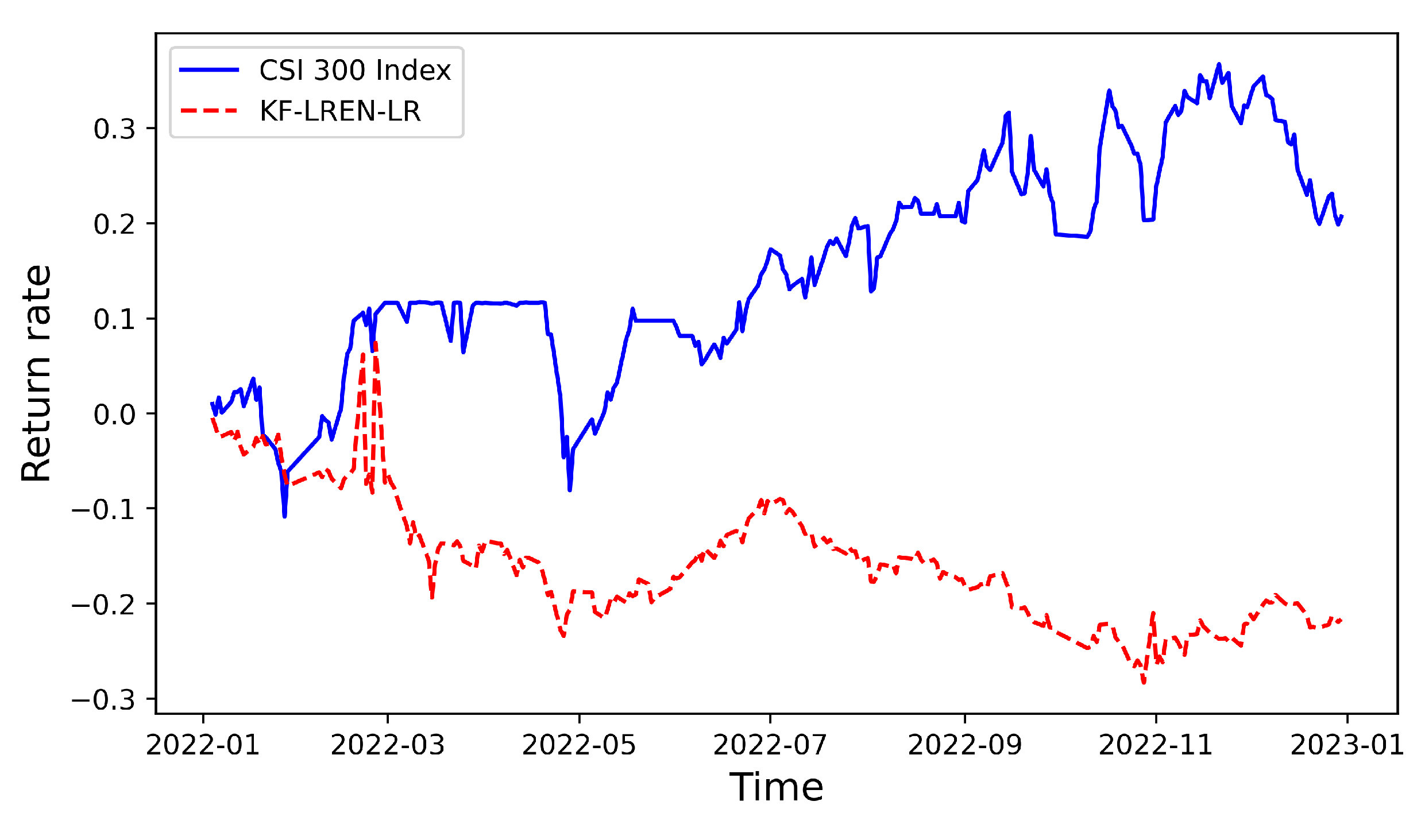
The performance of the multifactor stock-selection strategy established in this paper is shown in Figure 3 and Table 5 for a total of 242 trading days throughout the backtest period. Intuitively, the strategy return curve trend is more in line with the index trend, and the overall trend is relatively stable. At the investment return level, the cumulative return of the strategy portfolio exceeds the benchmark return, and most of the time, the strategy portfolio returns are above the benchmark cumulative return curve, indicating that the strategy is able to obtain stable excess returns. For the whole backtesting period, the KF-LREN-LR model constructed in this paper had high accuracy when it came to trend-category prediction. Compared with the −21.63% annualized return of the buy-and-hold CSI 300 index, the multifactor stock-selection strategy built in this paper not only exceeds the benchmark return but also achieves a positive return of 20.70% annualized, with a smaller maximum retracement of 17.67% and an Alpha coefficient of 0.30, indicating that the trading strategy is able to obtain a higher excess return.
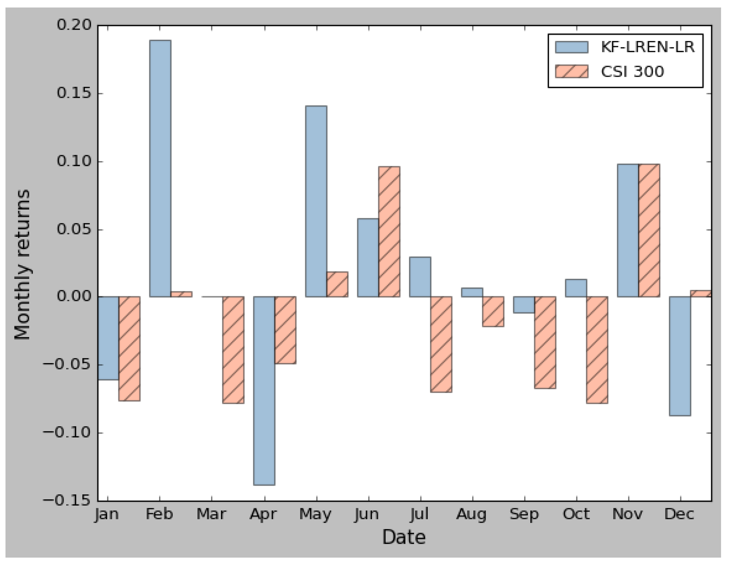
The analysis of Figure 3 shows that the multifactor stock-selection strategy established in this paper can achieve more stable excess returns when the overall price of the stock market rises or falls, and when the overall price shocks significantly, the corresponding portfolio will have a more obvious retracement of returns. The return chart shown in Figure 4 shows the profit and loss of the investment strategy on a monthly basis, reflecting the model’s ability to forecast and the profitability of the stock returns. In December, the KF-LREN-LR strategy had eight profitable months and only had a large loss in April, but the other profit levels were higher, and the highest profit level was higher than the maximum loss level, so it could obtain a higher cumulative total return.

3.4.2. Backtest Analysis of Multifactor Quantitative Stock-Selection Strategies under Different Market Environments

The backtesting period is selected to include time intervals with positive, negative, and oscillatory trends in order to more fully evaluate the efficacy of the multifactor stock-selection technique proposed in this research. The impact of the strategy is then compared to the buy-and-hold CSI 300 index on each of these three categories of time intervals.

3.4.3. Backtest Analysis in an Uptrend

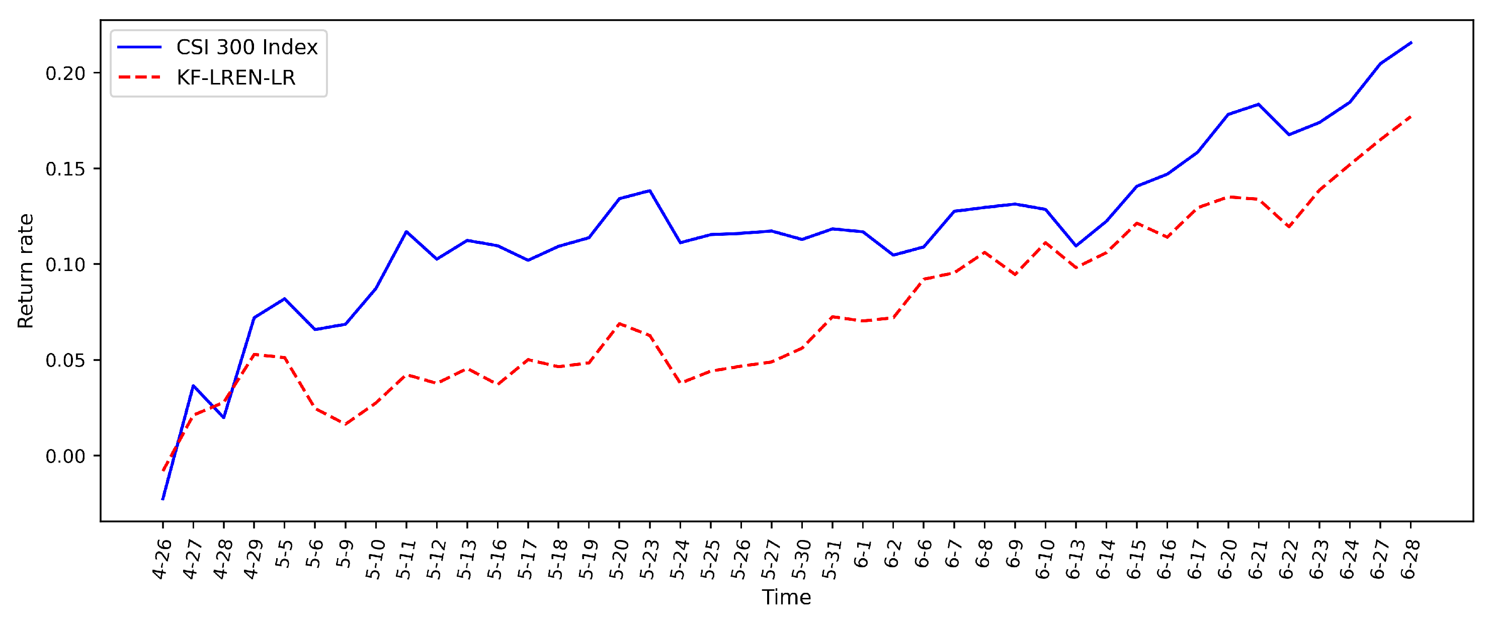
Figure 5 illustrates how this approach performed between 26 April 2022 and 28 June 2022, when the CSI 300 index showed an upward trend. Figure 5 and Table 6 show that the KF-LREN-LR model developed in this study performs well during this backtest period as it showed an increasing trend. The buy-and-hold CSI 300 index simple operation achieved a cumulative return of 17.71% due to good market conditions, and the multifactor stock-selection strategy established in this paper accurately predicted the price trend movement of each constituent stock in the backtesting period, eventually achieving a higher cumulative return of 21.56%, with a maximum retracement of only 2.96% in the uptrend phase, the lowest in the three environments. The Alpha coefficient is 0.6, which achieved a certain excess return in the case of a better return than the benchmark CSI 300 index, and the Beta coefficient is 0.97, which indicates that the variation in the trading strategy is smaller than that of the CSI 300 index, and the systematic risk is within the acceptable range. Finally, the results of the Sharpe ratio, winning percentage, profit and loss ratio, and information ratio are combined to show that the multifactor stock-selection strategy established in this paper performed better in terms of the return capture and risk control through a high winning percentage and high profit and loss ratio during the backtest period.

3.4.4. Backtest Analysis in a Downtrend

The performance of the strategy during the period from 4 July 2022 to 11 October 2022, when the CSI 300 index had a significant downward trend, is shown in Figure 6. As can be seen from Figure 6 and Table 6, the model was still relatively accurate at predicting the price movement trends of certain CSI 300 constituents. Due to the poor overall financial market, the buy-and-hold CSI 300 index operation resulted in a cumulative asset loss of 16.55%. When building the portfolio, the multifactor stock-selection strategy developed in this paper chooses a specific percentage of candidate stocks and accurately predicts the trend movements of the majority of the stocks. This tactic not only avoided a loss in the long run but also saw a return of 1.60%. The Beta coefficient is 0.79, which indicates that the trading strategy effectively controlled the systematic risk of its own return. Despite the fact that the winning percentage was only 0.46 because of the general stock market decline, the profit and loss ratio of 3.87 was able to partially offset the asset losses and manage risk.

3.4.5. Backtest Analysis in a Shock Trend

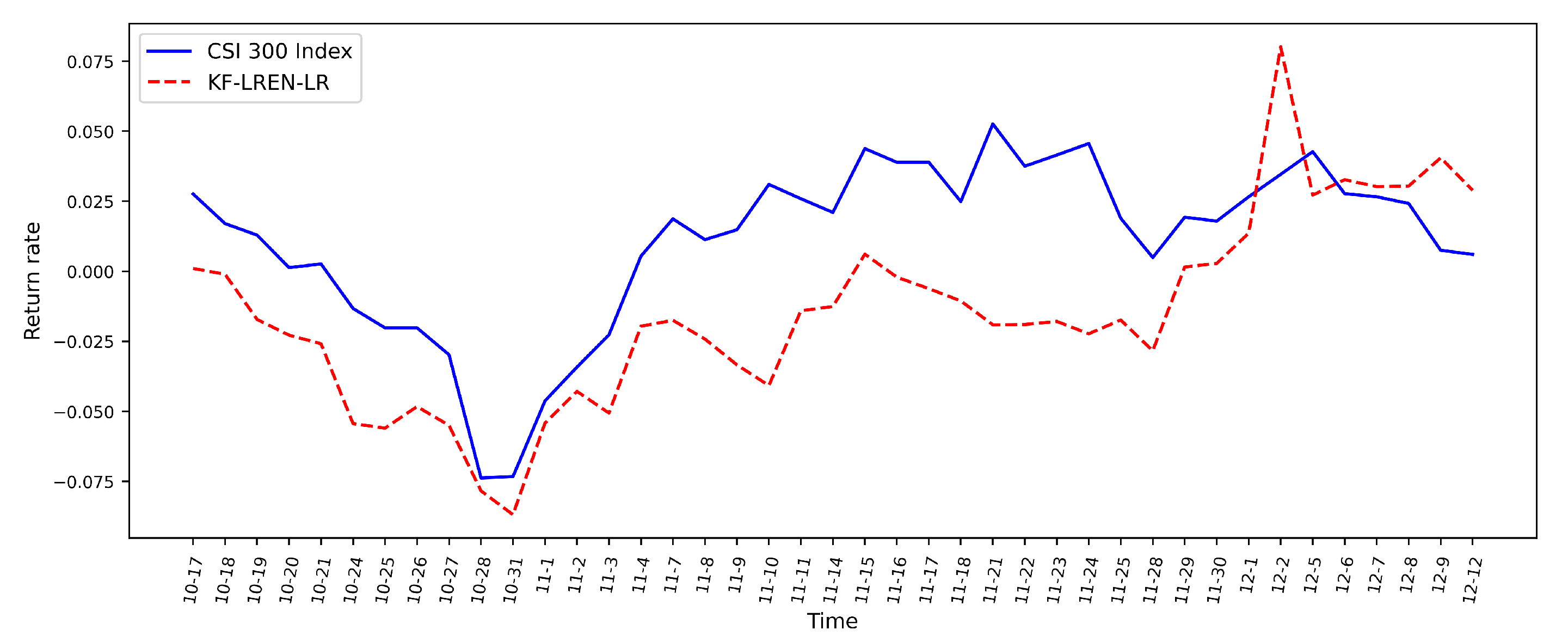
The performance of the strategy is shown in Figure 7 for the period from 17 October 2022 to 12 December 2022, a relatively oscillating period for the CSI 300 index. The time period includes the market changes after the National Day holiday and before Chinese New Year, and the market experienced a large fluctuation. The total assets of the buy-and-hold CSI 300 index increased by 2.89% as the market experienced a relatively oscillating trend, and the KF-LREN-LR of this paper only achieved an annualized return of 0.6% in the end. The maximum retracement is 9.87%, and the Alpha coefficient is only 0.09, which is not satisfactory when the annualized return of the benchmark buy-and-hold CSI 300 index is good but still positive. The systemic risk control is not as good as in the rising and falling phases. Finally, the results of the Sharpe ratio, winning percentage, profit and loss ratio, and information ratio show that the strategy established in this paper does not perform as well during the rising and falling phases in terms of both the return and risk during the backtesting period. Therefore, the KF-LREN-LR strategy is more capable of gaining returns and controlling risk when the index is falling or rising significantly.

4. Conclusions and Prospect

Based on the monthly data of the CSI 300 index constituents from January 2016 to December 2022, a portfolio model is constructed by using the KF-LR-Elastic Net variable-selection method and the Logistic-classification forecasting method. The effective factors with a relatively significant impact on the stock returns were selected from the original factor pool, and we controlled for the FDR; this was followed by forecasting whether the individual stock returns could outperform the CSI 300 index and constructing a portfolio for a historical trading backtest. The following conclusions are drawn:
First, the KF-LR-Elastic Net model is used to screen quantitative factor indicators with high explanatory power for returns. This method has a higher overlap with the other indicators selected by Elastic Net regression without the inclusion of Knockoff variables and Lasso-Logistic regression without Elastic Net regularization but tends to select fewer variables for the purpose of controlling false positives.
Second, Logistic regression is chosen as the forecasting model, and the forecasting model is built based on the selected factors. Logistic regression is used to predict stock returns, and it can construct a high-quality portfolio before and after the introduction of Knockoff, which can meet the needs of investors for proper risk avoidance. The results show that the Knockoff-based portfolios are more robust in terms of monthly returns alone. The model and strategy are more advantageous when there is a significant upward or downward trend in the stock market. By incorporating the Elastic Net rule, the Knockoff approach is able to construct a strategy with higher excess returns and lower risk.
Third, the relationship between quantitative factor indicators and stock returns is studied with an eye on the Chinese stock market. The application of Knockoff on multifactor stock selection was shown to have merit and can lead to a better investment performance, better serve investors’ decision making, and provide an intelligent investment-decision method.
In summary, this paper combines Knockoff, Elastic Net regularization, and Logistic regression. On the one hand, the method is significantly superior at selecting the factors that have a real and significant impact on obtaining the excess return of stocks among many candidate factors. On the other hand, the constructed KF-LREN-LR model can better explore the information about financial assets and select the assets with high returns, which is significant for stabilizing returns and controlling market risks. In addition, the methodology of this paper can be extended from multiple perspectives. In terms of models, Knockoff’s “counterfeit” idea can be extended to other models or methods, such as machine learning methods, including support vector machines, linear discriminant analysis, etc.; it can also be extended to methods of multisource data fusion, such as integration analysis, etc. In terms of variable-selection methods, the Lasso used in this paper can be replaced with other methods, especially when it comes to the variable-grouping structure. Variable selection can be achieved by using sparse-group MCP and CMCP penalties, etc. In terms of application, it can also be extended to practical problems such as credit default early warning and financial risk early warning, which are worth further exploration in subsequent research.

Author Contributions

Conceptualization, Y.R. and G.T.; methodology, Y.R.; software, Y.R.; validation, Y.R., G.T. and X.L.; formal analysis, Y.R.; investigation, Y.R.; resources, Y.R.; data curation, Y.R.; writing—original draft preparation, Y.R.; writing—review and editing, G.T.; visualization, X.C.; supervision, Y.R.; project administration, G.T.; funding acquisition, G.T. All authors have read and agreed to the published version of the manuscript.

Funding

This research was funded by the Natural Science Foundation of Guangxi (Grant No. 2022GXNSFAA035499) and the National Natural Science Foundation of China (62166015).

Data Availability Statement

The data that support the findings of this study are available from the corresponding author upon request.

Conflicts of Interest

The authors have no relevant financial or nonfinancial interests to disclose.

References

  1. Markowitz, H.M. Portfolio selection. J. Financ. 1952, 7, 77–91. [Google Scholar] [CrossRef]
  2. Sharpe, W.F. Capital asset prices: A theory of market equilibrium under conditions of risk. J. Financ. 1964, 19, 425–442. [Google Scholar] [CrossRef] [Green Version]
  3. Ross, S.A. The arbitrage theory of capital asset pricing. J. Econ. Theory 1976, 13, 341–360. [Google Scholar] [CrossRef]
  4. Fama, E.F.; French, K.R. Common risk factors in the returns on stocks and bonds. J. Financ. Econ. 1993, 33, 3–56. [Google Scholar] [CrossRef]
  5. Carhart, M.M. On persistence in mutual fund performance. J. Financ. 1997, 52, 57–82. [Google Scholar] [CrossRef]
  6. Fama, E.F.; French, K.R. A five-factor asset pricing model. J. Financ. Econ. 2015, 116, 1–22. [Google Scholar] [CrossRef] [Green Version]
  7. Stambaugh, R.F.; Yuan, Y. Mispricing factors. Rev. Financ. Stud. 2017, 30, 1270–1315. [Google Scholar] [CrossRef] [Green Version]
  8. Asness, C.S. The interaction of value and momentum strategies. Financ. Anal. J. 1997, 53, 29–36. [Google Scholar] [CrossRef]
  9. Fan, J.; Lv, J. A selective overview of variable selection in high dimensional feature space. Stat. Sin. 2010, 4, 101–148. [Google Scholar] [CrossRef] [Green Version]
  10. Hastie, T.; Tibshirani, R. Generalized Additive Models. Stat. Sci. 1986, 1, 297–318. [Google Scholar] [CrossRef]
  11. Lin, Y.; Zhang, H.H. Component selection and smoothing in multivariate nonparametric regression. Ann. Stat. 2006, 34, 2272–2297. [Google Scholar] [CrossRef] [Green Version]
  12. Chen, H.; Wang, Y.; Zheng, F.; Deng, C.; Huang, H. Sparse modal additive model. IEEE Trans. Neural Netw. Learn. Syst. 2020, 32, 2373–2387. [Google Scholar] [CrossRef] [PubMed]
  13. Tibshirani, R. Regression shrinkage and selection via the lasso. J. R. Stat. Soc. Ser. B 1996, 58, 267–288. [Google Scholar] [CrossRef]
  14. Yuan, M.; Lin, Y. Model selection and estimation in regression with grouped variables. J. R. Stat. Soc. Ser. B 2006, 68, 49–67. [Google Scholar] [CrossRef]
  15. Bach, F.R. Consistency of the group lasso and multiple kernel learning. J. Mach. Learn. Res. 2008, 9, 1179–1225. [Google Scholar] [CrossRef]
  16. Lemhadri, I.; Ruan, F.; Tibshirani, R. Lassonet: Neural networks with feature sparsity. Mach. Learn. Res. 2019, 130, 10–18. [Google Scholar] [CrossRef]
  17. Ravikumar, P.; Liu, H.; Lafferty, J.; Wasserman, L.A. SpAM: Sparse Additive Models. J. R. Stat. Soc. Ser. Stat. Methodol. 2009, 71, 1009–1030. [Google Scholar] [CrossRef]
  18. Zou, H.; Hastie, T. Regularization and variable selection via the elastic net. J. R. Stat. Soc. 2005, 67, 301–320. [Google Scholar] [CrossRef] [Green Version]
  19. Wang, X.C. Construction of quantitative trading intelligence System based on LASSO and neural network–Shanghai and Shenzhen 300 stock index futures as an example. Investig. Res. 2014, 33, 23–29. https://doi.org/CNKI:SUN:TZYJ.0.2014-09-003.
  20. Li, B.; Shao, X.; Li, Y. Research on fundamental quantitative investment driven by Machine learning. China’s Ind. Econ. 2019, 8, 61–79. [Google Scholar] [CrossRef]
  21. Shu, S.; Li, L. Regular sparse multi-factor quantitative stock selection Strategy. Comput. Eng. Appl. 2021, 10, 110–117. [Google Scholar] [CrossRef]
  22. Jagannathan, R.; Ma, T. Risk reduction in large portfolios: Why imposing the wrong constraints helps. J. Financ. 2003, 58, 1651–1683. [Google Scholar] [CrossRef] [Green Version]
  23. Benjamini, Y.; Hochberg, Y. Controlling the false discovery rate: A practical and powerful approach to multiple testing. J. R. Stat. Soc. Ser. B 1995, 57, 289–300. [Google Scholar] [CrossRef]
  24. Barber, R.F.; Candes, E.J. Controlling the False Discovery Rate Via Knockoffs. Ann. Stat. 2015, 43, 2055–2085. [Google Scholar] [CrossRef] [Green Version]
  25. Candes, E.; Fan, Y.; Janson, L.; Lv, J. Panning for gold: Model-x knockoffs for high-dimensional controlled variable selection. J. R. Stat. Soc. Ser. B Stat. 2018, 80, 551–577. [Google Scholar] [CrossRef] [Green Version]
  26. Fan, Y.; Demirkaya, E.; Lv, J. Nonuniformity of p-values can occur early in diverging dimensions. J. Mach. Learn. Res. 2019, 20, 2849–2881. [Google Scholar] [CrossRef]
  27. Gégout-Petit, A.; Gueudin-Muller, A.; Karmann, C. The revisited knockoffs method for variable selection in L 1-penalized regressions. Commun.-Stat.-Simul. Comput. 2020, 51, 5582–5595. [Google Scholar] [CrossRef]
  28. Katsevich, E.; Sabatti, C. Multilayer knockoff filter: Controlled variable selection at multiple resolutions. Ann. Appl. Stat. 2019, 13, 1–33. [Google Scholar] [CrossRef]
  29. Barber, R.F.; Candès, E.J. A knockoff filter for high-dimensional selective inference. Ann. Stat. 2019, 5, 2504–2537. [Google Scholar] [CrossRef]
  30. Liu, W.; Ke, Y.; Liu, J.; Li, R. Model-Free Feature Screening and F DR Control with Knockoff Features. J. Am. Stat. Assoc. 2022, 117, 428–443. [Google Scholar] [CrossRef]
  31. Dai, R.; Barber, R. The knockoff filter for FDR control in group-sparse and multitask regression. JMLR 2016, 47, 1851–1859. [Google Scholar] [CrossRef]
  32. Srinivasan, A.; Xue, L.; Zhan, X. Compositional knockoff filter for high-dimensional regression analysis of microbiome data. Biometrics 2021, 77, 984–995. [Google Scholar] [CrossRef] [PubMed]
  33. Zhu, G.; Zhao, T. Deep-gknock: Nonlinear group-feature selection with deep neural networks. Neural Networks. Neural Netw. 2021, 135, 139–147. [Google Scholar] [CrossRef] [PubMed]
  34. Hoerl, A.E.; Kennard, R.W. Ridge Regression: Applications to Nonorthogonal Problems. Technometrics 1970, 12, 69–82. [Google Scholar] [CrossRef]
  35. Boyd, S.; Vandenberghe, L. Convex Optimization, 1st ed.; Cambridge University Press: Cambridge, UK, 2004; pp. 127–189. [Google Scholar] [CrossRef]
  36. Zhang, H.; Shen, H.; Liu, Y. The study on multi-factor quantitative stock selection based on self-attention neural network. J. Appl. Stat. Manag. 2020, 29, 556–570. [Google Scholar] [CrossRef]
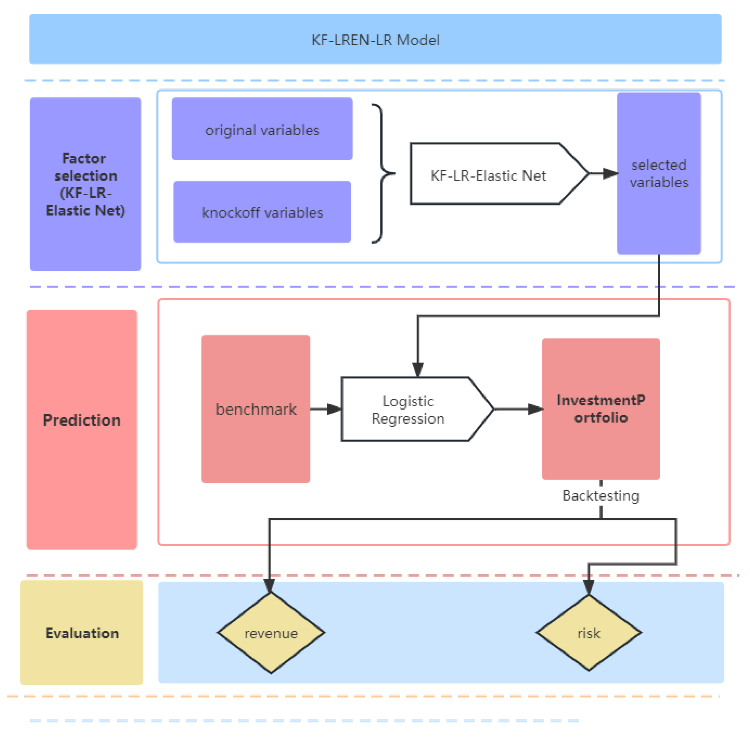
Figure 1. Model design structure chart.
Mathematics 11 03502 g001
Figure 2. Trend of CSI 300 index.
Mathematics 11 03502 g002
Figure 3. Returns of KF-LREN-LR during whole backtest.
Mathematics 11 03502 g003
Figure 4. Comparison of monthly returns during backtest.
Mathematics 11 03502 g004
Figure 5. Comparison of strategy returns in uptrend stage.
Mathematics 11 03502 g005
Figure 6. Comparison of strategy returns in downtrend stage.
Mathematics 11 03502 g006
Figure 7. Comparison of strategy returns during shock trend.
Mathematics 11 03502 g007
Table 1. ADF unit root test results.
TitleValue
Test Statistic−1.6165
p-value0.7407
Lags Used11
Number of observations used1703
Critical Value (1%)−3.2125
Critical Value (5%)−2.2354
Critical Value (10%)−2.1583
Table 2. Results of factor screening.
KF-LR-Elastic NetKF + -LR-Elastic NetLR-Elastic NetKF-LR-Lasso
PBPBPBPB
PEPEPEPE
--LFLOLFLO
ARTRate-ARTRateARTRate
GrossIncomeRatioGrossIncomeRatioGrossIncomeRatioGrossIncomeRatio
ROEROEROEROE
NetProfitGrowRateNetProfitGrowRateNetProfitGrowRateNetProfitGrowRate
FSALESGFSALESGFSALESGFSALESG
DVRATDVRATHBETADVRAT
SKEWSKEWSKEWSKEW
DDNBTDDNBTDDNBTDDNBT
---DDNSR
DDNSR-TOBTTOBT
FiftyTwoweekHighFiftyTwoweekHighFiftyTwoweekHighFiftyTwoweekHigh
EARNMOMEARNMOMEARNMOMEARNMOM
-MACDMACDMACD
HurstHurstHurstHurst
DHILODHILODHILODHILO
BIAS5BIAS5BIAS5BIAS5
VRVRVRVR
--ADXADX
GREVGREVGREVGREV
SFY12PSFY12PSFY12PSFY12P
GSREV--GSREV
--OBV6OBV6
Table 3. Logistic regression classification results based on different factor-selection models.
Prediction ModelFactor-Selection ModelAccuracyRecallPrecisionF1
LRKF-LR-Elastic Net75.45%71.55%75.30%73.38%
KF + -LR-Elastic Net75.48%71.56%75.37%73.42%
LR-Elastic Net74.35%70.86%72.84%71.84%
KF-LR-Lasso74.77%71.13%73.78%72.43%
Table 4. Classification results of different prediction models.
Factor-Selection ModelPrediction ModelAccuracyRecallPrecisionF1
KF-LR-Elastic NetLR75.45%71.55%75.30%73.38%
SVM74.44%70.92%73.04%71.96%
RF74.45%70.93%73.07%71.99%
LSTM75.31%71.46%74.98%73.18%
Table 5. KF-LREN-LR backtest effect evaluation table.
IndexAnnual Rate of ReturnCSI 300 ReturnBetaInformation RatioSharpe
Value21.45%−21.63%0.481.520.61
IndexWinning percentageProfit and loss ratioAlphaMaximum pullback
Value0.532.090.3017.67%
Table 6. Comparison of backtest results across three categories of time periods.
CategoryUpDownVolatile
Backtest period4.26–6.287.4–10.1110.17–12.30
Benchmark return17.71−16.552.89
Tactics return21.561.860.60
Annual rate of return219.717.243.74
Beta0.970.790.55
Alpha0.600.460.09
Sharpe ratio8.330.12−0.01
Winning percentage0.750.460.40
Profit and loss ratio5.143.871.79
Information ratio3.052.40−0.66
Maximum pullback2.969.929.87
Disclaimer/Publisher’s Note: The statements, opinions and data contained in all publications are solely those of the individual author(s) and contributor(s) and not of MDPI and/or the editor(s). MDPI and/or the editor(s) disclaim responsibility for any injury to people or property resulting from any ideas, methods, instructions or products referred to in the content.