Article

Modeling Software Reliability with Learning and Fatigue

by
Tahere Yaghoobi
1,* and
Man-Fai Leung
2
1
Department of Computer Engineering and Information Technology, Payame Noor University, Tehran 19395-4697, Iran
2
School of Computing and Information Science, Faculty of Science and Engineering, Anglia Ruskin University, Cambridge CB1 1PT, UK
*
Author to whom correspondence should be addressed.
Mathematics 2023, 11(16), 3491; https://doi.org/10.3390/math11163491
Submission received: 28 June 2023 / Revised: 8 August 2023 / Accepted: 10 August 2023 / Published: 13 August 2023
(This article belongs to the Section Mathematics and Computer Science)

Abstract

:
Software reliability growth models (SRGMs) based on the non-homogeneous Poisson process have played a significant role in predicting the number of remaining errors in software, enhancing software reliability. Software errors are commonly attributed to the mental errors of software developers, which necessitate timely detection and resolution. However, it has been observed that the human error-making mechanism is influenced by factors such as learning and fatigue. In this paper, we address the issue of integrating the fatigue factor of software testers into the learning process during debugging, leading to the development of more realistic SRGMs. The first model represents the software tester’s learning phenomenon using the tangent hyperbolic function, while the second model utilizes an exponential function. An exponential decay function models fatigue. We investigate the behavior of our proposed models by comparing them with similar SRGMs, including two corresponding models in which the fatigue factor is removed. Through analysis, we assess our models’ quality of fit, predictive power, and accuracy. The experimental results demonstrate that the model of tangent hyperbolic learning with fatigue outperforms the existing ones regarding fit, predictive power, or accuracy. By incorporating the fatigue factor, the models provide a more comprehensive and realistic depiction of software reliability.

1. Introduction

Due to the ubiquitous use of software in our daily lives, accurately predicting the number of software errors has become crucial, particularly in critical applications. Software reliability growth models (SRGMs) based on the non-homogeneous Poisson process (NHPP) have emerged as widely adopted tools for this purpose [1] (Pham, 2006). These models allow for the numerical estimation of the remaining errors in software and provide insights into its reliability. To address the complexities of the software development process, SRGMs have evolved to incorporate various factors, including the experience, skill, and learning of software developers [2].
Research has highlighted the significant impact of fatigue on the human error-making process [3]. In particular, studies have demonstrated that fatigue can trigger attention switching in individuals, typically occurring after approximately 40 min of continuous activity. This fatigue-induced attention shift is attributed to a gradual reduction in dopamine secretion, eventually reaching a threshold that disrupts attention. Furthermore, it has been observed that other neurotransmitters cannot adequately compensate for the decline in dopamine release. To capture this phenomenon, researchers have modeled the decrease in dopamine secretion rate as an exponential decay process towards a specific limit [3].
Software debugging is the process of identifying and removing errors or defects in a computer program, which affects software reliability. Achieving perfect software debugging is often challenging and may not always be possible due to the inherent complexity of software development. The goal is to minimize bugs and deliver a high-quality product by employing best practices and continuously improving the development and debugging processes. In imperfect debugging, software testers inadvertently introduce new faults during the debugging process. Whether the debugging process is perfect or imperfect can be influenced by various human-related and non-human-related factors, such as the experience and skill of debuggers, debugging tools, program size and complexity, testing strategies, and environmental factors [4]. We believe that learning and fatigue are two human-related factors that can significantly impact software debugging, influencing the efficiency and effectiveness of the process. The reason is that developers familiar with the codebase, understand the software’s logic and expected behavior, and possess domain knowledge to understand the intricacies and potential pitfalls can do more efficient debugging.
On the other hand, debugging requires sustained attention and focus, as developers need to analyze code, identify patterns, and devise solutions. Fatigue can lead to reduced concentration, making it easier to overlook critical details or commit errors during debugging. Debugging can be time-consuming and sometimes frustrating, especially when dealing with complex bugs. Fatigue may reduce a developer’s patience and persistence, potentially resulting in prematurely abandoning the problem-solving process or the hasty application of inadequate fixes. In both cases, learning and fatigue can work hand in hand. New developers or those less familiar with the codebase may experience increased fatigue as they need to invest more effort in understanding the code and identifying issues. Conversely, fatigue can hinder the learning process, making it more challenging for developers to absorb new information (experience) or gain deeper insights into the software.
This research delves into a new specific aspect of imperfect debugging, i.e., the impact of tester fatigue on the debugging process. We assume these imperfections can stem from attention-switching problems caused by tester fatigue. Understanding that fatigue can lead to attention-switching problems and subsequently introduce new defects is crucial for creating more accurate representations of real-world scenarios. This research introduces two SRGMs involving human-related factors of tester learning and fatigue. The first model represents the software tester’s learning phenomenon via the tangent hyperbolic (tanh) function, while the second model utilizes an exponential function. We investigate the behavior of our proposed models by comparing them with similar SRGMs, including the corresponding two perfect software reliability models that do not consider the effect of the fatigue factor. We estimate the models’ parameters and assess their fit, predictive abilities, and accuracy using three datasets to validate them.
Section 2 of this paper focuses on reviewing the relevant literature and exploring previous works in the field. Section 3 introduces the mathematical formulations of our proposed models, which are based on a general framework of a family of SRGMs. Section 4 presents numerical examples to illustrate the application and performance of the models. To gain a deeper understanding of the proposed models, Section 5 conducts a sensitivity analysis, providing valuable insights into their behavior and critical parameters. Finally, Section 6 concludes this paper, summarizing the main findings and highlighting our research contributions.

2. Literature Review

2.1. Learning Curves

Learning refers to acquiring new knowledge, skills, or understanding, and a learning curve visually represents the relationship between skill level, expertise, and the time required to complete a task. Mathematically, learning can be described using various functions, each representing different improvement patterns over time. Three typical learning curves are S-shaped, exponential, and exponential growth to a limit. The S-shaped learning curve demonstrates the initial exponential growth, followed by a period of slower growth and ultimately approaching a maximum upper limit that is never fully reached. The logistic function commonly describes an S-shaped learning curve, also known as the sigmoid curve. The exponential learning curve illustrates a slow rate of progress at the beginning, gradually increasing over time until full proficiency is achieved. Unlike the S-shaped curve, the exponential learning curve suggests that learning can improve indefinitely without limits. The exponential growth to a limit learning curve indicates that initial attempts result in rapid skill acquisition or information retention, reaching a maximum rate and approaching a maximum upper limit. However, perfection or significant improvement in the skill may not occur with subsequent repetitions. Figure 1 represents three standard types of learning curves.

2.2. Related Works

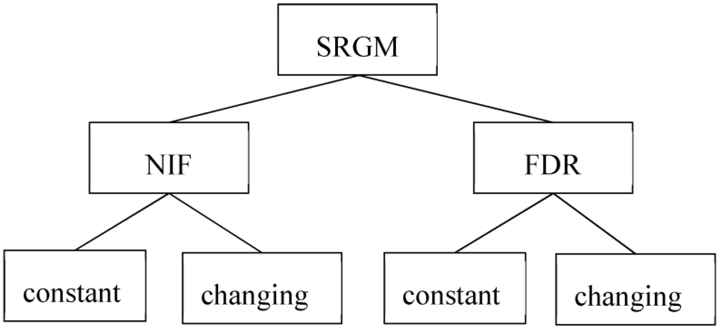
Over the past few decades, researchers have made significant advancements in developing software reliability growth models by exploring various ideas and approaches. One notable contribution in this field is the work of Pham and Nordmann, who introduced a general framework for constructing new SRGMs [5]. This framework has served as a foundation for interpreting several existing software reliability models. Within this framework, two concepts play vital roles in the construction of an SRGM: the expected number of initial faults (NIF) present in the software at the beginning of the testing phase and the fault detection rate (FDR), which represents the rate at which failures are detected over time. In the context of software debugging, both NIF and FDR can be treated as either constant or varying in a time-dependent manner. Figure 2 categorizes this group of SRGMs based on whether the NIF and FDR are considered constant or subject to change. This figure helps to provide a clearer understanding of the different models within this family.
In models with constant NIF, it is assumed that when a fault is detected, it is immediately removed by the testers, and no new errors are introduced in the process. Consequently, the software’s initial defects remain unchanged throughout the debugging phase. On the other hand, in software reliability models with changing NIF, it is acknowledged that new faults may be introduced during the testing phase. This means that the total number of defects in the software is not constant and comprises both the initial faults and the additional faults introduced during the debugging process. This assumption recognizes the possibility of testers unintentionally introducing new errors while attempting to fix existing defects.
The FDR is a significant indicator of the effectiveness of the testing phase. It is influenced by various factors, including the expertise of testers, testing techniques employed, and the selection of test cases. The FDR can remain constant or vary among faults depending on the software reliability model. In the case of a constant FDR, it is assumed that all defects in the software have an equal probability of being detected throughout the testing period. This implies that the FDR remains consistent over time, irrespective of the specific characteristics of the faults.
Conversely, in models with a time-dependent FDR, the function may exhibit increasing or decreasing trends as time progresses. This variation acknowledges the dynamic nature of the testing process, where the effectiveness of fault detection can be influenced by factors such as the testing team’s expertise, the program’s size, and the software’s testability. By incorporating the concept of a changing FDR, software reliability models can better reflect the complexities and uncertainties inherent in real-world testing scenarios. Recognizing the dependence of the FDR on various factors enables researchers to develop more accurate models and gain deeper insights into the dynamics of software reliability assessment.
A. 
SRGMs with constant NIF and constant/changing FDR
The Goel–Okumoto model [6] is a widely referenced example of an NHPP model with constant NIF and FDR. More SRGMs with constant NIF and changing FDR have been proposed in the literature. These models consider learning phenomena, time resources, testing coverage, and environmental uncertainties. Yamada et al. [7] introduced the concept of a learning process in software testing, where testers gradually improve their skills and familiarity with the software products. They formulated an increasing FDR with a hyperbolic function to represent the learning rate of testers and proposed the delayed S-shaped model. Ohba [8] considered the learning process of testers during the testing phase and defined the FDR using a non-decreasing logistic S-shaped curve, leading to the development of the inflection S-shaped model. Yamada and Osaki [9] considered the consumption of time resources and proposed the exponential testing effort and Rayleigh testing effort models. Pham [1] introduced the imperfect fault detection (IFD) model, which incorporates a changing FDR that combines fault introduction with the phenomenon of testing coverage. This model allows for a more realistic representation of the testing process. Song et al. [10] considered the impact of testing coverage uncertainty or randomness in the operating environment. They proposed a new NHPP software reliability model with constant NIF and changing FDR regarding a testing coverage function, considering the uncertainty associated with operational environments.
B. 
SRGMs with changing NIF and constant/changing FDR
More SRGMs with time-dependent changing NIF function and constant/changing FDR have been proposed in the literature. For example, Yamada et al. [11] proposed two imperfect debugging models assuming the NIF function to be an exponential or linear function of the testing time, respectively, and FDR to be constant. Pham and Zhang [12] developed an imperfect debugging model considering an exponential function of testing time for NIF and a non-decreasing S-shaped function for FDR. Pham et al. [13] proposed an imperfect SRGM with NIF function to be linear and FDR S-shaped of the testing time. Li and Pham [14] introduced a new, changing NIF model, and FDR is expressed as a testing coverage function. In their model, they also assumed that when a software failure is detected, immediate debugging starts, and either the total number of faults is reduced by one with probability p or the total number of faults remains the same with probability 1-p.
C. 
Other SRGMs
Many imperfect SRGMs do not fit the above framework precisely and use other approaches. For example, Chiu et al. [15] proposed a model that considers the influential factors for finding errors in software, including the autonomous errors-detected and learning factors. They proposed an FDR function including two factors representing the exponential-shaped and the S-shaped types of behaviors. Iqbal et al. [16] investigated the impact of two learning effect factors: autonomous and acquired learning, which are gained after repeated experience/observation of the testing/debugging process by the tester/debugger in an SRGM. Wang et al. [17] proposed an imperfect software debugging model that considers a log-logistic distribution function for NIF, which can capture the increasing and decreasing characteristics of the fault introduction rate per fault. They reason imperfect software debugging models proposed in the literature generally assume a constantly or monotonically decreasing fault introduction rate per fault. These models cannot adequately describe the fault introduction process in a practical test. Wang and Wu [18] proposed a nonlinear NHPP imperfect software debugging model by considering that fault introduction is a nonlinear process. Al-Turk and Al-Mutairi [19] developed an SRGM based on one-parameter Lindley distribution, which is modified by integrating two learning effects of the autonomous error-detected factor and the learning factor. These studies highlight the ongoing efforts to refine SRGMs by considering real-world scenarios and addressing the critical aspects of the software testing and debugging processes. Huang et al. [20] developed an NHPP model considering both human factors (learning effect of the debugging process) and the nature of errors, such as varieties of errors and change points, during the testing period to extend the practicability of SRGMs. Verma et al. [21] proposed an SRGM by considering conditions of error generation, fault removal efficiency (FRE), imperfect debugging parameter, and fault reduction factor (FRF). The error generation, imperfect debugging, and FRE parameters have been assumed to be constant, while FRF is time dependent and modeled using exponential, Weibull, and delayed s-shaped distribution functions. Luo et al. [22] recently proposed a new SRGM with a changing NIF and FDR represented by an exponential decay function of testing time.
Each category of SRGMs has its own set of advantages and disadvantages. On one end of the spectrum, SRGMs with a changing NIF and FDR tend to have more parameters, as they incorporate various assumptions to yield a more realistic representation of the underlying processes. However, this realism comes at the cost of increased complexity. Complex models may require more resources, such as time and memory, to appropriately evaluate. While the abundance of parameters offers flexibility, it also leads to higher computational overhead.
In contrast, SRGMs with a constant NIF and FDR follow a simpler approach, resulting in fewer parameters and more straightforward models. A simpler model is generally easier to comprehend, interpret, and implement. Despite potentially sacrificing some level of realism, the simplicity of such models can prove advantageous, especially when computational efficiency and ease of use are significant considerations.

3. Development of New NHPP Software Reliability Models

This study focuses on modeling SRGMs with a constant NIF and time-dependent FDR function. This choice has two reasons: (1) To gain a deeper insight into how the new time-dependent FDR affects the model’s behavior. By focusing on the FDR function, we aim to understand its implications in software reliability analysis. (2) Simplicity is another objective of this approach. Employing a constant NIF makes the resulting model more straightforward to interpret. Simpler models are often favored for their ease of implementation and comprehensibility.
The mean value function, m t , for the class of NHPP-SRGMs with a constant NIF and time-dependent FDR function, can be obtained by solving the following differential equation:
d m ( t ) d t = r t · a m t with   m 0 = 0
in which a > 0 is the NIF, i.e., the number of defects in the software at the beginning of the test, and r t is a time-dependent FDR function that denotes the rate of discovering new faults in software over the testing. The SRGM defined via Equation (1) is based on the following assumptions: (1) a non-homogeneous Poisson process can describe the fault removal process; (2) the faults that remained in the software caused system failures at random times; (3) the mean number of detected faults is proportional to the mean number of remaining faults in the system. By introducing various functions for r t , which can be interpreted as different assumptions made, the mathematical expression for m t can be derived. For example, when r t = b , then m t = a [ 1 exp b t ] , which is the GO model [6].
Now, we propose new models based on Equation (1) by considering the following functions for r(t):
  • The combination of tanh learning with fatigue;
  • The combination of exponential learning with fatigue;
  • Tanh learning without fatigue;
  • Exponential learning without fatigue.
This study analyzes two learning curves: one based on the tanh function and the other based on the exponential function. The objective is to determine which curve more accurately captures the actual learning behavior in the context of this research. Unlike previous studies that have usually used an S-shaped curve for modeling r t , this research introduces a novel approach by adopting the tanh t function, where t ≥ 0, which exhibits an exponential-to-limit behavior for learning. Furthermore, this study explores the integration of this new learning curve with the fatigue phenomenon to model r t . The behavior of the two proposed models is also investigated when the fatigue factor is removed from the models.
In model NEW1, we assume r t represents a weighted combination of the tanh learning with the fatigue of the tester as follows:
r t = α tanh s t + β e w t
Parameters s and w represent the learning and fatigue rates, respectively. α and β are positive coefficients representing the weights of each factor. By substituting Equation (2) in Equation (1) and solving the resulting differential equation, the mathematical form of the mean value function of the NEW1 model is obtained as follows:
m t = a [ 1 e β e w t 1 w c o s h α s s t ]
This model assumes that each time a failure is observed, the failure is removed, and new faults can be introduced due to fatigue.
In model NEW2, we assume r t is the combination (for simplicity, average) of exponential learning and fatigue.
r t = k cosh s t
Parameter s represents an equal rate of learning and fatigue, and k is a weight. By substituting Equation (4) in Equation (1) and solving the resulting differential equation, the mathematical form of the mean value function of model NEW2 is obtained as follows:
m t = a 1 e k s i n h s t s
In model NEW3, only the tanh learning function without the fatigue factor is considered for r t as follows:
r t = k · tanh s t
By substituting Equation (6) in Equation (1) and solving the resulting differential equation, the mathematical form of the mean value function of model NEW3 is obtained as follows:
m t = a [ 1 c o s h k s s t ]
In model NEW4, only the exponential learning function without the fatigue factor is considered for r t as follows:
r t = k e s t
By substituting Equation (8) in Equation (1) and solving the resulting differential equation, the mathematical form of the mean value function of model NEW4 is obtained as follows:
m t = a [ 1 e k 1 e s t s ]

4. Numerical Examples

Our experiments specifically considered SRGMs that align with this modeling framework, featuring constant NIF and either constant or changing FDR. Table 1 summarizes the characteristics of the similar existing SRGMs and the proposed models used in this study.

4.1. Descriptions of the Datasets

Three datasets from different real software projects have been used to study our proposed models’ fitting and predictive ability, validate our approaches, and compare them with similar ones. The first dataset (DS1) is Release 1 of the Tandem Computers Software Data Project. Over 20 weeks, 100 faults were detected [23]. This dataset is frequently used in the literature. The second dataset (DS2) was obtained from a real-time command and control system. During 25 h, 136 faults were detected [1]. The third dataset (DS3) was collected from a wireless network switching system. Over 34 weeks, 181 defects were detected [24]. Table 2 briefly describes three datasets used in this study.

4.2. Criteria for Model Comparison

We employed three criteria to compare and illustrate the models’ fitting, predictive capabilities, and accuracy. These criteria were chosen to provide comprehensive evaluations of the models’ performance. The three criteria used are outlined as follows.
Criterion 1. (A measure of fit)
The mean squared error (MSE) is a widely used criterion to assess the adequacy of a software reliability model’s fit. Given a dataset consisting of pairs of observed failure times ( t i , m i ) for i = 1, 2,…, k, where k represents the total number of observations in the dataset, the MSE quantifies the discrepancy between the predicted values of the model and the corresponding actual data. Mathematically, the MSE is defined as follows:
M S E = 1 k i = 1 k [ m i m t i ] 2
m i denotes the cumulated number of actual software failures found until the time t i , and m ( t i ) is the model estimate for the cumulated number of failures discovered at the time t i . A smaller value of the MSE criterion represents a minor error in fitting and therefore indicates a better model performance.
Criterion 2. (A measure of prediction)
The predictive ability of a software reliability growth model refers to its capability to predict future and unseen software failure data based on the observed failure data. The predictive ratio risk (PRR) is a criterion to assess the model’s prediction accuracy. It quantifies the discrepancy between the model’s estimations and the actual observations. The PRR is calculated as follows [25]:
PRR = i = 1 k [ m t i m i m t i ] 2
A smaller PRR indicates a better performance of the model.
Criterion 3. (A measure of accuracy)
Theil’s statistic (TS) measures accuracy, assessing the deviation between the actual values and the model’s predictions across all periods. It is calculated as the average deviation and is defined as follows:
T S = i = 1 k m t i m i 2 i = 1 k m i 2
A closer T S to zero indicates better accuracy of the model.

4.3. Comparisons

To compare the proposed models’ fitting, predictive, and accuracy with other models, we divided the datasets into two subsets: 80% and 20%. The 80% subset was used to estimate the parameters of the models using the least-square error method. These estimated parameter values were then applied to the 80% subset to calculate the mean square error (MSE_fit) values. The estimated parameter values were also applied to the remaining 20% of the datasets to calculate the predictive ratio risk (PRR_predict) values. Finally, the estimated parameter values were used for the entire period of collected failure data to calculate Theil’s statistic (TS) values, which measure accuracy.
(1)
DS1 (Tandem dataset).
Table 3 displays the optimal parameter values for each SRGM and the corresponding values obtained via the MSE_fit, PRR_predict, and TS criteria using the DS1 dataset.
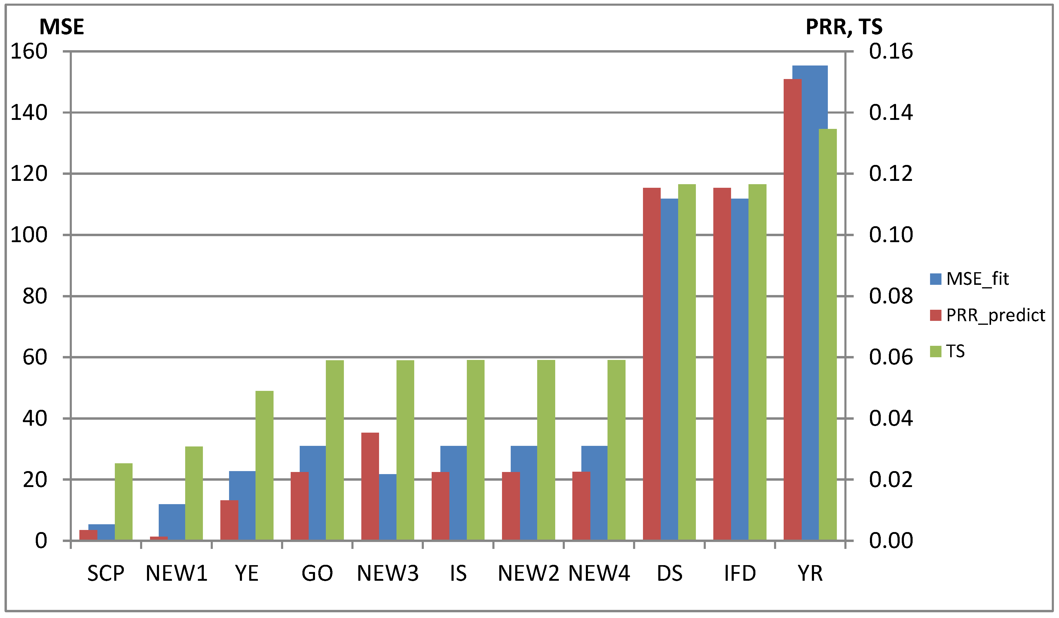
Figure 3 represents the values obtained from Table 3 in a combo chart.
Based on the fitting ability (MSE_fit), the NEW1 model, which incorporates tanh learning and fatigue, demonstrates the highest fitting level to the DS1 dataset. Regarding predictive power (PRR_predict), the NEW1 model exhibits minimal prediction errors and outperforms other models. When considering the measure of accuracy (TS), the NEW1 model emerges as the most precise. Additionally, the other proposed models exhibit commendable performance compared to competing models.
A comparative analysis of the four proposed models shows that the NEW1 model (incorporating tanh learning with fatigue) outperforms its counterparts across all three evaluation criteria. Concerning the models’ fitting ability, NEW2 (employing exponential learning with fatigue) exhibits superior performance compared to NEW4 (utilizing exponential learning alone), followed by NEW3 (applying tanh learning). Regarding predictive power, NEW3 slightly surpasses NEW2, while NEW4 demonstrates the least favorable predictive performance. Regarding accuracy, NEW2 outperforms NEW3, followed by NEW4 as the least accurate model.
Table 4 presents the estimated number of defects projected in the proposed models.
(2)
DS2 (Real-time and Command dataset)
Table 5 displays the optimal parameter values for each SRGM and the corresponding values obtained via the MSE_fit, PRR_predict, and TS criteria using the DS2 dataset.
Figure 4 represents the values obtained from Table 5 in a combo chart.
Based on the fitting ability (MSE_fit), the SCP model demonstrates the best fit, followed by the NEW1 model for the DS2 dataset. Regarding predictive power (PRR_predict), the NEW1 model exhibits the lowest prediction errors, while the SCP model ranks second. Regarding accuracy (TS), the NEW1 model is the second-most accurate model after SCP. The other proposed models exhibit satisfactory performance and outperform the DS, IFD, and YR models.
A comparative analysis of the four proposed models shows that the NEW1 model (incorporating tanh learning with fatigue) outperforms its counterparts across all three evaluation criteria. NEW2 (employing exponential learning with fatigue) and NEW4 (utilizing exponential learning alone) exhibit considerable similarity in their performance across all three criteria. Meanwhile, the NEW3 model, which applies tanh learning, showcases distinct characteristics compared to NEW2 and NEW4. It notably excels in fitting ability; however, its predictive power falls behind that of NEW2 and NEW4, suggesting that NEW3 might be less accurate in making future predictions. Nevertheless, in terms of accuracy, NEW3 performs similarly to NEW2 and NEW4, implying that all three models yield comparable levels of correctness in their predictions.
Table 6 presents the estimated number of defects for the proposed models.
(3)
DS3 (Wireless network system dataset)
Table 7 displays the optimal parameter values for each SRGM and the corresponding values obtained via the MSE_fit, PRR_predict, and TS criteria using the DS3 dataset.
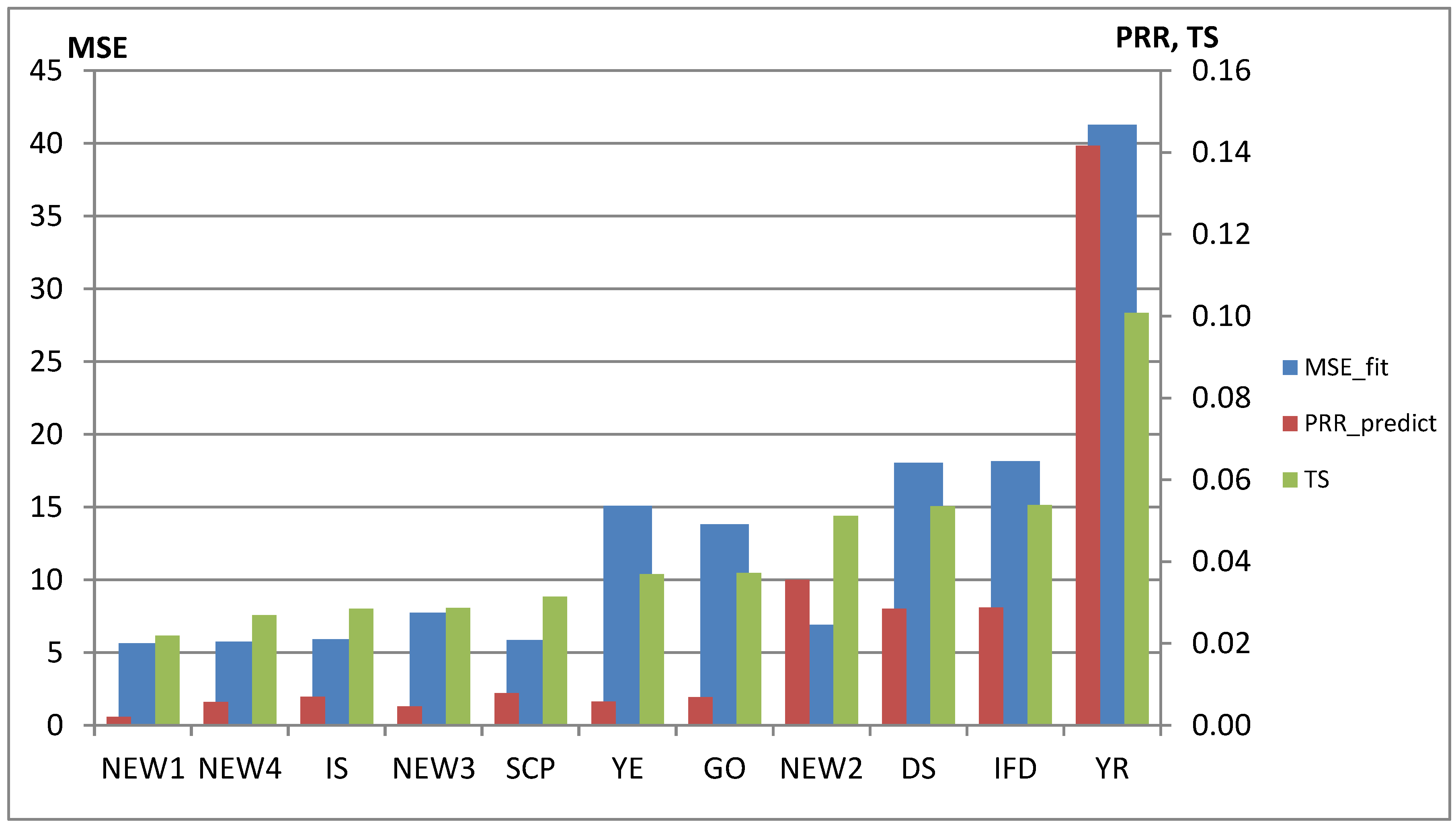
Figure 5 represents the values obtained from Table 7 in a combo chart.
Based on the fitting ability (MSE_fit), the NEW1 model best fits the DS3 dataset. Regarding predictive power (PRR_predict), the NEW1 model exhibits the lowest prediction errors. Regarding accuracy (TS), the NEW1 model is the most accurate. The other proposed models also exhibit satisfactory performance among their competitors.
In a comparative analysis of the four proposed models, compelling evidence emerges, clearly showcasing the superiority of the NEW1 model (integrating tanh learning with fatigue) over its counterparts across all three evaluation criteria. Conversely, NEW2 (employing exponential learning with fatigue) exhibits the least favorable performance among all models, showcasing inferior results across all three criteria. Furthermore, NEW4 (utilizing exponential learning exclusively) demonstrates advantages over NEW3 (applying tanh learning) regarding fitting ability and accuracy. However, it falls short compared to NEW3 regarding predictive power, implying that NEW3 possesses a better capability to make accurate future predictions.
Table 8 presents the estimated number of defects for the proposed models.

4.4. Threats to the Validity

In this section, we address potential limitations to the generalizability of our findings. These limitations primarily concern the applicability of our models in industrial settings. Although our experiments utilized three real datasets to demonstrate the performance of the proposed models, it is essential to acknowledge that the results may vary across specific applications. The reason is that software reliability models rely on the failure dataset; thus, no single model is suitable for every application. Furthermore, the choice of criteria and models used in the experiments is another issue that may impact the outcomes. We selected three comparison criteria and seven competitor models based on previous software reliability studies that align with our approach. We recommend using additional criteria and expanding the set of candidate models for evaluation and comparison to select the most suitable software reliability model for a specific application. Expanding the evaluation’s scope can give a more comprehensive understanding of the models’ performance.

5. Sensitivity Analysis

A scientific model can be likened to a black box that takes inputs and produces corresponding outputs. In the case of a mathematical model, sensitivity analysis is employed to assess the impact of changes in input values on the model’s outputs. Sensitivity analysis serves various purposes, including prioritizing model inputs to identify the critical drivers of model behavior. It also provides insights into the stability of inputs. Sensitivity plots visualize how the model’s output changes when the inputs are modified within predetermined small ranges. This information is valuable for managers, decision-makers, or analysts as it offers insights into the problem. In one-way sensitivity analysis, inputs are varied individually around a selected value of interest, and the variations can be minor. By systematically adjusting the parameter values, we gained insights into the model’s response to parameter changes and identified the parameters significantly impacting the model’s behavior.
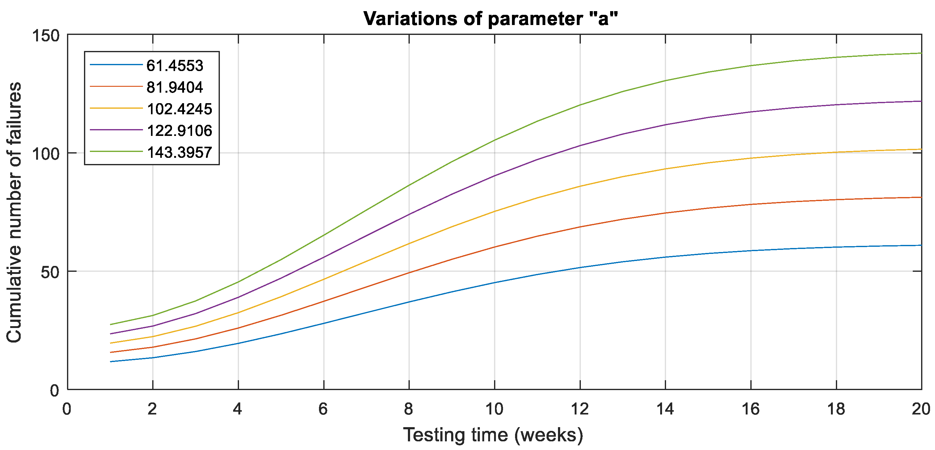
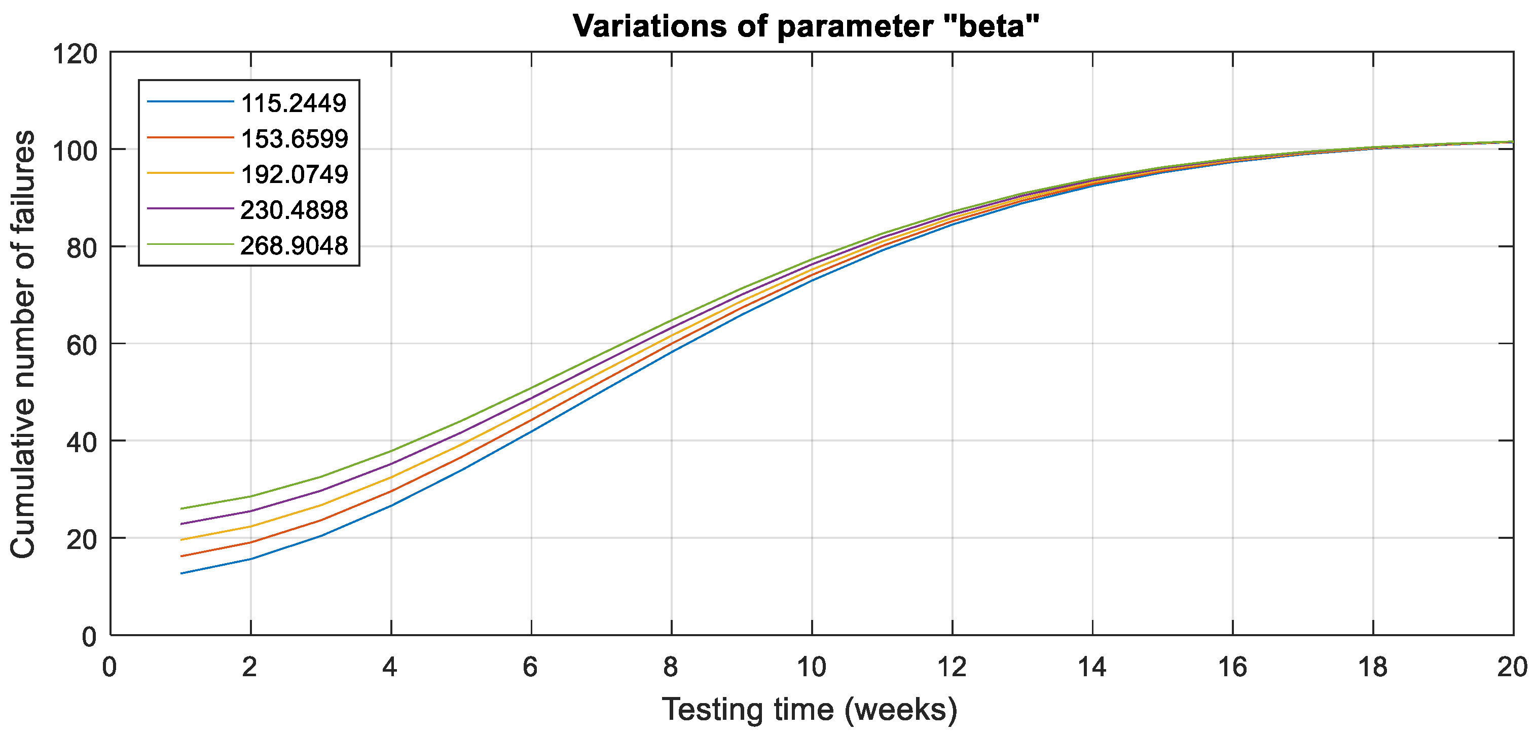
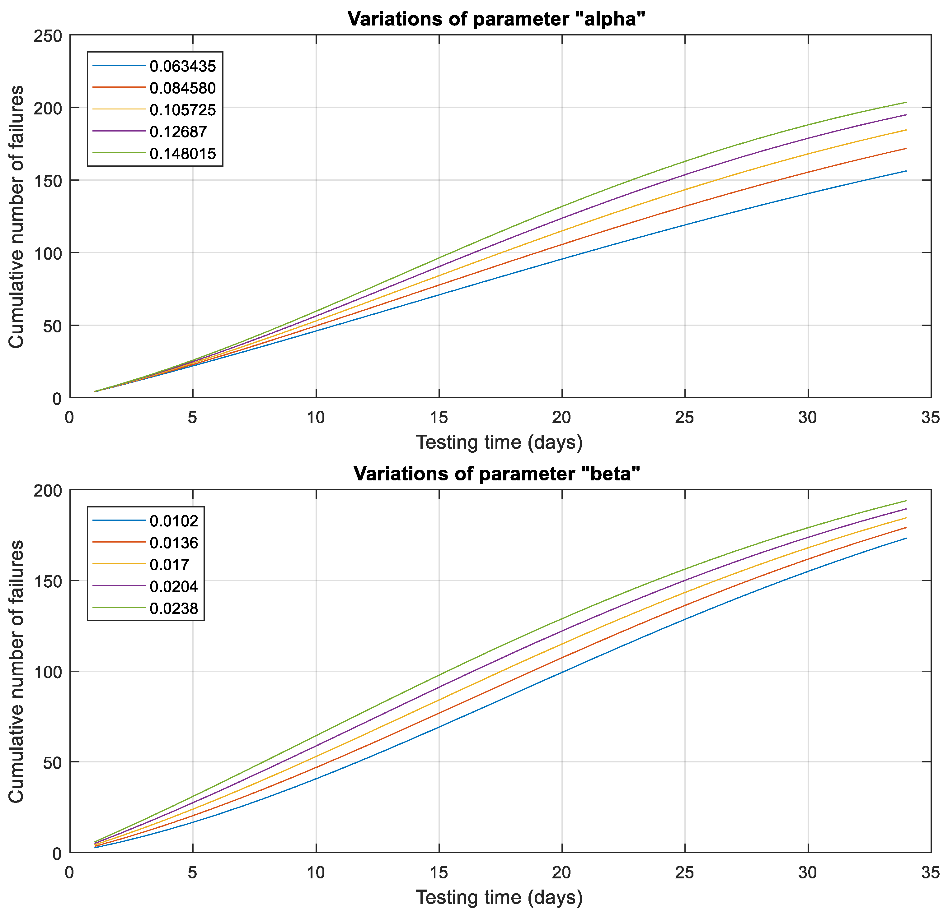
To assess the sensitivity and stability of the NEW1 model, we conducted a one-way sensitivity analysis by modifying a single parameter while keeping all other parameters fixed. This analysis aimed to identify which model parameters are sensitive to changes and which are more stable. Specifically, we examined how variations in the estimated parameter values obtained from Table 3, Table 5 and Table 7, ranging from −40% to +40% at 20% intervals, affect the estimated mean value function of the NEW1 model.
In Figure 6, Figure 7 and Figure 8, we present the results of a sensitivity analysis performed on all five parameters of the NEW1 model, utilizing DS1-DS3 datasets. These figures display the mean value function, m(t), for the NEW1 model. Within each figure, we vary one parameter value, as represented in the corresponding plots, while keeping the remaining parameters fixed, following the details in Table 3, Table 5 and Table 7. These figures provide insights into the impact of parameter variations on the cumulative number of expected faults. It is evident from Figure 6, Figure 7 and Figure 8 that among all parameters of the NEW1 model, the predicted number of initial defects, represented by the parameter “a”, plays a critical role in driving the behavior of the proposed model. Parameter changes “a” result in noticeable variations in the model’s output for all datasets.
Figure 6 also reveals that slight changes in parameter “s”, corresponding to the learning rate, lead to slight changes in the model’s output. Parameter “w”, corresponding to the fatigue factor, remains stable, indicating that the model’s output is less sensitive to these parameter changes. Similarly, slight changes in the value “α” lead to minor modifications in the model’s output, and weight “β” indicates the robustness of the variations.
Figure 7 demonstrates that variations in parameter “s” has no impact on the value of the NEW1 model, reaffirming its stability. Changes in parameters “w” and “β” do not result in noticeable modifications to the model’s output. However, the slight parameter variations in “α” lead to slight model value fluctuations. Overall, the sensitivity analyses highlight the significance of the predicted number of initial defects (parameter “a”) in driving the behavior of the NEW1 model. Parameters “w”, “s”, and “β” are considered stable and robust, while parameter “α” exhibit relatively minor effects on the model’s output.
Figure 8 illustrates the sensitivity analysis results of the NEW1 model using DS3. It can be observed that the parameter “w” exhibits stability, meaning that variations in its value have a minimal impact on the model’s overall value. On the other hand, changes in the parameters “s”, “α” and “β” lead to minor fluctuations in the model’s value.
Similar sensitivity analyses can be performed for other models using a similar approach.

6. Conclusions

In this study, we aimed to develop a novel software reliability model that integrates two critical human-related factors: learning and fatigue of software debuggers. While existing research has examined the impact of learning and experience on software reliability, there is a noticeable gap in the literature concerning the study of other human-related factors, such as fatigue. This work considered fatigue’s effects on error making, incorporating fatigue as a crucial factor in constructing the software reliability model. The findings presented in this paper demonstrate the robust performance of the model across all the datasets examined, showcasing its efficacy in predicting software reliability. By employing the tanh function to represent learning and the exponential decay function to model fatigue, we have contributed to the existing knowledge in this field. The successful application of these functions to represent the FDR highlights their suitability for capturing the dynamics of human-related factors in the reliability estimation process. Despite the promising results, it is essential to acknowledge the limitations and constraints of our study. The unavailability of new datasets restricted our ability to test the model on more recent datasets. However, the older datasets are still relevant and valid in understanding the underlying principles in the current studied domain, as researchers widely use them.
Additionally, the choice of the FDR function was constrained to ensure the solvability of the resulting differential equation. For future research, we recommend exploring the development of alternative models that incorporate other factors affecting fault introduction. By considering a more comprehensive set of variables, we can further enhance the accuracy and applicability of software reliability models.

Author Contributions

Conceptualization, T.Y. and M.-F.L.; software, T.Y. and M.-F.L.; formal analysis, T.Y. and M.-F.L.; data curation, T.Y. and M.-F.L.; writing—original draft preparation, T.Y. and M.-F.L.; writing—review and editing, T.Y. and M.-F.L. All authors have read and agreed to the published version of the manuscript.

Funding

This research received no external funding.

Data Availability Statement

Data availability is not applicable to this article as no new data were created or analyzed in this study.

Conflicts of Interest

The authors declare no conflict of interest.

References

  1. Pham, H. System Software Reliability. Reliability Engineering Series; Springer: London, UK, 2006. [Google Scholar]
  2. Yamada, S. Software Reliability Modeling: Fundamentals and Applications; Springer: Tokyo, Japan, 2014; Volume 5. [Google Scholar]
  3. Baghdadi, G.; Jafari, S.; Sprott, J.C.; Towhidkhah, F.; Golpayegani, M.H. A chaotic model of sustaining attention problems in attention deficit disorder. Commun. Nonlinear Sci. Numer. Simul. 2015, 20, 174–185. [Google Scholar] [CrossRef]
  4. Zhang, X.; Pham, H. An analysis of factors affecting software reliability. J. Syst. Softw. 2000, 50, 43–56. [Google Scholar] [CrossRef]
  5. Pham, H.; Nordmann, L. A generalized NHPP software reliability model. In Proceedings of the 3rd Int’l Conference on Reliability and Quality in Design, Anaheim, CA, USA, 12–14 March 1997; pp. 116–120. [Google Scholar]
  6. Goel, A.L.; Okumoto, K. Time-dependent error-detection rate model for software reliability and other performance measures. IEEE Trans. Reliab. 1979, 28, 206–211. [Google Scholar] [CrossRef]
  7. Yamada, S.; Ohba, M.; Osaki, S. S-shaped reliability growth modeling for software error detection. IEEE Trans. Reliab. 1983, 32, 475–484. [Google Scholar] [CrossRef]
  8. Ohba, M. Inflection S-Shaped Software Reliability Growth Model. In Stochastic Models in Reliability Theory. Lecture Notes in Economics and Mathematical Systems; Osaki, S., Hatoyama, Y., Eds.; Springer: Berlin/Heidelberg, Germany, 1984; Volume 235. [Google Scholar]
  9. Yamada, S.; Osaki, S. Software reliability growth modeling: Models and applications. IEEE Trans. Softw. Eng. 1985, 12, 1431–1437. [Google Scholar] [CrossRef]
  10. Song, K.Y.; Chang, I.H.; Pham, H. A testing coverage model based on NHPP software reliability considering the software operating environment and the sensitivity analysis. Mathematics 2019, 7, 450. [Google Scholar] [CrossRef] [Green Version]
  11. Yamada, S.; Tokuno, K.; Osaki, S. Imperfect debugging models with fault introduction rate for software reliability assessment. Int. J. Syst. Sci. 1992, 23, 2241–2252. [Google Scholar] [CrossRef]
  12. Pham, H.; Zhang, X. An NHPP software reliability model and its comparison. Int. J. Reliab. Qual. Saf. Eng. 1997, 4, 269–282. [Google Scholar] [CrossRef]
  13. Pham, H.; Nordmann, L.; Zhang, Z. A general imperfect-software-debugging model with S-shaped fault-detection rate. IEEE Trans. Reliab. 1999, 48, 169–175. [Google Scholar] [CrossRef]
  14. Li, Q.; Pham, H. A testing-coverage software reliability model considering fault removal efficiency and error generation. PLoS ONE 2017, 12, e0181524. [Google Scholar] [CrossRef] [PubMed] [Green Version]
  15. Chiu, K.C.; Huang, Y.S.; Lee, T.Z. A study of software reliability growth from the perspective of learning effects. Reliab. Eng. Syst. Saf. 2008, 93, 1410–1421. [Google Scholar] [CrossRef]
  16. Iqbal, J.; Ahmad, N.; Quadri, S.M.K. A software reliability growth model with two types of learning. In Proceedings of the 2013 International Conference on Machine Intelligence and Research Advancement, Katra, India, 21–23 December 2013; pp. 498–503. [Google Scholar]
  17. Wang, J.; Wu, Z.; Shu, Y.; Zhang, Z. An imperfect software debugging model considering log-logistic distribution fault content function. J. Syst. Softw. 2015, 100, 167–181. [Google Scholar] [CrossRef]
  18. Wang, J.; Wu, Z. Study of the nonlinear imperfect software debugging model. Reliab. Eng. Syst. Saf. 2016, 153, 180–192. [Google Scholar] [CrossRef]
  19. Al-Turk, L.I.; Al-Mutairi, N.N. Enhancing reliability predictions by considering learning effects based on one-parameter Lindley distribution. In Proceedings of the 2020 IEEE Asia-Pacific Conference on Computer Science and Data Engineering, Gold Coast, Australia, 16–18 December 2020; pp. 1–7. [Google Scholar]
  20. Huang, Y.S.; Chiu, K.C.; Chen, W.M. A software reliability growth model for imperfect debugging. J. Syst. Softw. 2022, 188, 111267. [Google Scholar] [CrossRef]
  21. Verma, V.; Anand, S.; Kapur, P.K.; Aggarwal, A.G. Unified framework to assess software reliability and determine optimal release time in the presence of fault reduction factor, error generation and fault removal efficiency. Int. J. Syst. Assur. Eng. Manag. 2022, 13, 2429–2441. [Google Scholar] [CrossRef]
  22. Luo, H.; Xu, L.; He, L.; Jiang, L.; Long, T. A Novel Software Reliability Growth Model Based on Generalized Imperfect Debugging NHPP Framework. IEEE Access 2023, 11, 71573–71593. [Google Scholar] [CrossRef]
  23. Wood, A. Software Reliability Growth Models; TANDEM Technical Report; Tandem Computers: Cupertino, CA, USA, 1996; Volume 96. [Google Scholar]
  24. Jeske, D.R.; Zhang, X.; Pham, L. Adjusting software failure rates that are estimated from test data. IEEE Trans. Reliab. 2005, 54, 107–114. [Google Scholar]
  25. Pham, H.; Deng, C. Predictive-ratio risk criterion for selecting software reliability models. In Proceedings of the 9th International Conference on Reliability and Quality in Design, Honolulu, HI, USA, 7–9 August 2003; pp. 17–21. [Google Scholar]
Figure 1. Learning curves of S-shaped, exponential, and exponential to a limit.
Mathematics 11 03491 g001
Figure 2. A classification of some SRGMs.
Mathematics 11 03491 g002
Figure 3. Combo chart representing MSE, PRR, and TS values for SRGMs using DS1.
Mathematics 11 03491 g003
Figure 4. Combo chart representing MSE, PRR, and TS values for SRGMs using DS2.
Mathematics 11 03491 g004
Figure 5. Combo chart representing MSE, PRR, and TS values for SRGMs using DS3.
Mathematics 11 03491 g005
Figure 6. Sensitivity analysis plots for the parameters of the NEW1 model using DS1.
Mathematics 11 03491 g006aMathematics 11 03491 g006bMathematics 11 03491 g006c
Figure 7. Sensitivity analysis plots for the parameters of the NEW1 model using DS2.
Mathematics 11 03491 g007aMathematics 11 03491 g007b
Figure 8. Sensitivity analysis plots for the parameters of the NEW1 model using DS3.
Mathematics 11 03491 g008aMathematics 11 03491 g008b
Table 1. Characteristics of SRGMs used in this study.
Model m t r ( t ) Comments
Goel-Okumoto (GO) a ( 1 e b t ) b Constant FDR [6]
Delayed
S-shaped (DS)
a [ 1 1 + b t e b t ] b 2 t 1 + b t Increasing FDR with a hyperbolic function [7]
Inflection S-shaped (IS) a 1 e b t 1 + c e b t b 1 + c e b t Increasing FDR with a two-parameter logistic function [8]
Yamada Exponential (YE) a [ 1 e r α 1 e β t ] r α β e β t Proportional to the exponential testing effort function [9]
Yamada Rayleigh (YR) a [ 1 e α r 1 e β t 2 2 ] r α β t e β t 2 2 Proportional to the Rayleigh testing effort function [9]
IFD a a e b t [ 1 + b + d t + b d t 2 ] b 2 t 1 + b t d 1 + d t Combination of a testing coverage with a fault introduction rate function [1]
SCP a [ 1 β β + b t ln 1 + d t ] α η ( d + 1 + d t b ) 1 + d t e b t Testing coverage with the uncertainty of the operating environment (η has a generalized probability density function with two parameters α and β.) [10]
NEW1 a [ 1 e β e w t 1 w c o s h α s s t ] α . tanh s t + β . e w t Combination of tanh learning with fatigue (Current study)
NEW2 a [ 1 e k s i n h s t s ] k . cosh s t Average of exponential learning with fatigue (Current study)
NEW3 a [ 1 c o s h k s s t ] k . tanh s t Tanh learning (Current study)
NEW4 a [ 1 e k 1 e s t s ] k . e s t Exponential learning (Current study)
Table 2. Summary of the selected failure data sets.
Data SetTesting PeriodCumulative Number of Failures
DS1Tandem Computer Software20 weeks100
DS2Real-time Command and Control System25 h136
DS3Wireless Network System34 days181
Table 3. Obtained results using DS1.
ModelMSE_FitPRR_PredictTSParameters
GO7.62460.0290360.065128a = 158.7887, b = 0.0624
DS31.2960.000740.067117a = 103.0886, b = 0.2684
IS7.62470.029020.065114a = 158.7224, b = 0.0625, c = 0.001
YE7.62860.03090.066846a = 178.2258, r = 0.01, α = 560.4812, β = 0.01
YR49.7350.0073460.087492a = 99.5568, r = 0.01, α = 398.3805, β = 0.01
IFD31.2990.000740.067122a = 103.0871, b = 0.2684, d = 0.00001
SCP6.63260.0517620.083567a = 443.5951, b = 611.657, d = 7.727, α = 0.1, β = 0.8235
NEW12.43460.0003210.019395a = 102.4245, s = 0.0001, w = 955.9065, α = 225.0417, β = 192.0749
NEW26.45890.00283460.034402a = 104.4743, k = 0.0954, s = 0.12998
NEW315.8870.00239590.049836a = 121.2902, k = 0.1, s = 2.0804
NEW47.62330.0274770.063675a = 149.458, k = 0.0659, s = 0.0064
Table 4. Comparison of the estimated defects by the new models using DS1.
Testing Time (Weeks)Defects FoundEstimated Defects by the NEW1 ModelEstimated Defects by the NEW2 ModelEstimated Defects by the NEW3 ModelEstimated Defects by the NEW4 Model
1162010810
22422181919
32727272827
43332343735
54139424543
64947495250
75454565956
85862626562
96969697068
107575747574
118181808079
128686858484
139090898788
149393939093
159696969397
1698989996100
17999910198104
18100100102101107
19100101103103110
20100101104104113
Table 5. Obtained results using DS2.
ModelMSE_FitPRR_PredictTSParameters
GO30.9050.022430.0589a = 128.9073, b = 0.156
DS111.770.115360.1165a = 116.1565, b = 0.418
IS30.9090.0224360.0590a = 128.9051, b = 0.156, c = 0.00017
YE22.7110.013260.0489a = 183.9655, r = 0.09, α = 14.9442, β = 0.09
YR155.360.150890.1346a = 116.9754, r = 0.025, α = 145.7865, β = 0.025
IFD111.770.115370.1165a = 116.1561, b = 0.418, d = 0.00001
SCP5.43060.0035720.025238a = 433.4581, b = 1000, d = 2.5449, α = 4.9218, β = 0.38695
NEW111.9860.00133610.0307a = 143.9516, s = 15.59059, w = 873.0036, α = 0.1, β = 138.7975
NEW230.9050.0224310.0590a = 128.9058, k = 0.156, s = 0.001
NEW321.6750.0352370.05892a = 123.4075, k = 0.169, s = 47.3651
NEW430.9410.0224930.0590a = 128.8742, k = 0.156, s = 0.00015
Table 6. Comparison of the estimated defects by the new models using DS2.
Testing Time (Hours)Defects FoundEstimated Defects by the NEW1 ModelEstimated Defects by the NEW2 ModelEstimated Defects by the NEW3 ModelEstimated Defects by the NEW4 Model
12732191919
24343353535
35453484948
46461606160
57569707070
68276787978
78483868686
88989929192
99294979697
109399102101102
1197103106104106
12104107109107109
13106110112110112
14111114114112114
15116116117114117
16122119118123118
17122121120123120
18127124121123121
19128126122123122
20129127123123123
21131129124123124
22132130125123125
23134132125123125
24135133126123126
25136134126123126
Table 7. The obtained results using DS3.
ModelMSE_FitPRR_PredictTSParameters
GO13.8230.00683110.0372a = 5724.2965, b = 0.001
DS18.050.0284930.0535a = 201.7278, b = 0.0977
IS5.9120.00701250.028491a = 208.1097, b = 0.1, c = 4.097
YE15.0720.0057750.0369a = 2989.2663, r = 0.1523, α = 84.755, β = 0.00015
YR41.2880.141660.1008a = 156.15498, r = 0.2652, α = 18396.9465, β = 0.0000015
IFD18.1630.0288240.0538a = 201.4796, b = 0.098, d = 0.0001
SCP5.85680.00782770.031415a = 964.07144, b = 18.663, d = 0.3086, α = 1.268, β = 1622.9581
NEW15.62620.00201310.0219a = 242.957, s = 0.017, w = 0.017, α = 0.1057, β = 0.017
NEW26.89760.0356030.0512a = 166.1322, k = 0.0322, s = 0.1017
NEW37.74250.0046374 0.028717a = 685.335, k = 0.01, s = 0.4079
NEW45.7540.00564390.0269a = 187.6476, k = 0.0237, s = 0.063
Table 8. Comparison of the estimated defects by the proposed models using DS3.
Testing Time (Days)Defects FoundEstimated Defects by the NEW1 ModelEstimated Defects by the NEW2 ModelEstimated Defects by the NEW3 ModelEstimated Defects by the NEW4 Model
154515
2691059
31314161014
42219211619
52424262324
62929312930
73435363535
84041414241
94647474847
105353535553
116359586159
127065646765
137172707371
147478777978
157884838584
169090909190
179897969797
18105103103103103
19110109109109109
20117115116115115
21123121122120121
22128127128126127
23130132133131133
24136138139137138
25141143144142143
26148149148148148
27156154152153153
28164159155158157
29166163158164161
30169168160169165
31170172162174168
32176177163179172
33180181164184174
34181185165189177
Disclaimer/Publisher’s Note: The statements, opinions and data contained in all publications are solely those of the individual author(s) and contributor(s) and not of MDPI and/or the editor(s). MDPI and/or the editor(s) disclaim responsibility for any injury to people or property resulting from any ideas, methods, instructions or products referred to in the content.