Abstract
In this work, a generalization of the Timoshenko beam theory is introduced, which is based on fractal continuum calculus. The mapping of the bending problem onto a non-differentiable self-similar beam into a corresponding problem for a fractal continuum is derived using local fractional differential operators. Consequently, the functions defined in the fractal continua beam are differentiable in the ordinary calculus sense. Therefore, the non-conventional local derivatives defined in the fractal continua beam can be expressed in terms of the ordinary derivatives, which are solved theoretically and numerically. Lastly, examples of classical beams with different boundary conditions are shown in order to check some details of the physical phenomenon under study.
Keywords:
Timoshenko beam; fractal beam; fractal calculus; fractional dimensions; transversal displacement MSC:
74S40
1. Introduction
Fractional operators have become indispensable tools in the analysis of physical and technological problems. The success of this approach is due to the fact that they present a better description of the phenomenon under study and allow solving functions that are not differentiable in the ordinary calculus sense.
To model the scale invariance of complex systems in the real world as a continuum body, two popular alternatives are often applied: fractional calculus [1,2,3,4,5,6], which uses a standard measure on the length scale where ordinary calculus is no longer valid, and fractal continuum calculus -CC [7,8,9,10,11], which uses non-standard measures like the Hausdorff measure [12,13,14,15] and incorporates fractional dimensions and fractal properties to characterize a fractal set.
Accordingly, significant efforts have been made by researchers and engineers to describe physical phenomena on fractal domains. Specifically, they have focused on stresses and strains in beams with complex geometries using ordinary [16,17,18], fractional [19,20,21,22,23], and fractal continuum calculus [24,25,26,27].
In this regard, Carpinteri’s beam is a mathematical model consisting of the Cartesian product of the Cantor set and the Sierpinski carpet that was suggested by Carpinteri et al. [28] to idealize inhomogeneous structures [29,30,31]. It is a classical example of the product measure framework suggested in [10,32] as a methodology for analysis in the fractal continuum calculus sense.
The product measure was developed to model anisotropic fractal media [33], which are characterized by different Hausdorff dimensions in the fractional directions (in some cases, as in the Cantor dusts [34]), transforming them into a parallelepiped with lengths . A modified product measure was presented by Balankin [35], which is a generalized version of the previous fractal continuum model. This new approach includes a particular fractional norm, metric, and measure, as well as vector differential calculus and a proper Laplacian. Therefore, it can be effectively applied to path-connected fractals [36]. Consequently, , where is the Hausdorff dimension of the shorter path on the fractal, and , where is the Hausdorff dimension of mass, while denotes the Hausdorff dimension of the cross-section area of the fractal. It should be noted that the fractal distances in the fractal continuum can be written in terms of Cartesian coordinates . Another modification of the product measure was introduced by Tarasov [37], whereas in [38], this framework was updated.
Many practical applications in the real world have been addressed using the original and modified versions of the product measure, for example, fluid flow [39,40] seismology [41], wave propagation [10,42], viscoelasticity [43], fracture mechanics [24,44], and electric fields [37]. Consequently, in [34], the concept of a fractal continuum beam was introduced to address structural problems in self-similar beams, referred to as Balankin’s beams.
In this work, a new fractal formulation of the Timoshenko beam theory within the -CC framework is proposed. The efficiency and accuracy of the proposed equations are demonstrated through graphs depicting the structural response of both Carpinteri’s and Balankin’s beams along their lengths.
This paper is organized as follows. We present the mathematical foundations of -CC in Section 2. In Section 3, the fractal Timoshenko beam theory is explained. In Section 4, the proposed formulation is applied to beams with various geometries and fractal topologies, and the structural details are discussed. The main conclusions are summarized in Section 5.
2. Terminology and Notations
In this section, first, the -CC framework is summarized, and then Carpinteri’s and Balankin’s beams are reviewed.
2.1. Fractal Continuum Calculus, -CC
The present technique involves creating a homogenized continuum model using a fractal metric mapping from a fractal domain , constructed in Euclidean space with Cartesian coordinates , to a fractal continuum domain in fractional coordinates (see Figure 1).
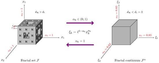
Figure 1.
Fractal set and its counterpart fractal continuum .
There are two types of fractals that can be mapped from to . The first type occurs when is totally disconnected, which is constructed as a Cartesian product. This implies that becomes a parallelepiped with lengths , density , and mass [10,38], whose Hausdorff dimension is given by , where is the Hausdorff dimension in each fractional spatial coordinate embedded in Euclidean space . The difficulties with implementing the Hausdorff dimension for numerical applications motivate the development of empirical estimates such as box-counting [13], packing [12], Hall-Wood [45], and two-scale transform [46], which are frequently used. On the other hand, the second type of fractal occurs when is a path-connected fractal, which means that its chemical dimension is equal to its Hausdorff dimension , and the number of its independent coordinates is <3. In contrast, the infinitesimal volume element in -CC is given by , where and are the infinitesimal area elements on the intersection between and a two-dimensional plane normal to the k-axis and , respectively. is the density of admissible states in the plane of this intersection, and .
Consequently, the measure in is defined by the following relations: , , and . Furthermore, -CC has the following local fractional differential operators [34,44,47]:
- -
- The fractional norm is given by , where , and the mapping of the fractional coordinates in the fractal continuum to the integer coordinates in the embedding Euclidean space is defined as
- -
- The distance between two points is given as , where .
- -
- The fractal gradient operator is , where and .
- -
- The divergence operator is .
- -
- The Laplacian is .
2.2. Fractal Beams
In this manuscript, two kinds of fractal beams are considered, whose geometries and fractal topologies are characterized by their Hausdorff, chemical, and elastic backbone () dimensions. For the beams studied here, : (i) Carpinteri’s beams, which are fractal sets constructed as Cartesian products [28], and (ii) Balankin’s beams [34], which are self-similar fractals with a path-connected structure, including the Menger sponge type and its modifications.
2.2.1. Carpinteri’s Beam
Carpinteri’s beam, , is the Cartesian product of the Cantor set and the Sierpinski carpet . The cross-sectional shape of this beam is the Sierpinski carpet, which is relatively smaller than its length defined by the Cantor set. It is embedded in Euclidean space, and it can be denoted using spatial coordinates, (see Figure 2a,b). The Cantor middle- set can be built by iteratively removing open middle- segments from the remaining segments of the previous iteration, starting from the unit interval . The Sierpinski carpet is obtained through an iterative process applied to the unit square . This square is divided into sub-squares of equal size, and the interior of sub-squares are deleted through multiple iterations. The Hausdorff dimensions of these fractals are defined by [48]
where d is the dimension of the embedding Euclidean space, is the number of boxes covering the fractal mass, is the number of deleted boxes of the fractal mass, and , defines the Hausdorff dimension of the Cantor middle- set and the classical Sierpinski carpet, respectively. Note that in the above equation can also be computed using the two-scale transform approach [46] with results identical to those of box-counting.
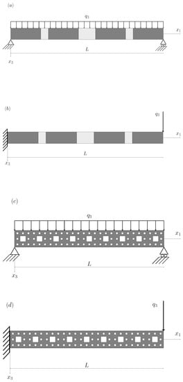
Figure 2.
Fractal beams with two different boundary conditions: (a) Carpinteri’s simply supported beam for , (b) Carpinteri’s cantilever beam for , (c) Balankin’s simply supported beam for , and (d) Balankin’s cantilever beam for .
It is easy to see that the Hausdorff dimension of the cross-sectional area of the beam is equal to the Hausdorff dimension of the Sierpinski carpet, denoted as . On the other hand, the Hausdorff dimension of Carpinteri’s beam is given by , where is the Hausdorff dimension along the fractional axes to which Carpinteri’s beam can be mapped.
2.2.2. Balankin’s Beam
Balankin’s beam , is part of the i-th iteration of the Menger sponge and is built using n sub-cubes of smaller iterations along the -axis, as depicted in Figure 2c,d. Here, all iterations share the same value of but possess different length scales of self-similarity . So, the Hausdorff dimension of Balankin’s beam is equal to that of the Menger sponge, and its cross-sectional area forms the Sierpinski carpet within the -plane. Additionally, the Hausdorff dimensions of their fractional axes are defined as .
Note that the Menger sponge is a 3D version of the Cantor set, which can be constructed by taking the unit cube and dividing it into cubes of equal size. Then, the interiors of the cubes are removed. In each of the remaining cubes, the same operation is repeated ad infinitum. Therefore, the value of for the Menger sponge can be computed using Equation (2) when .
3. Fractal Timoshenko Beam Equations
Timoshenko’s bending theory for a fractal continuum map is explained in this section, which is based on the principle of virtual work.
Timoshenko Beam Equations in -CC
The governing equations in the regime of elastostatics with the assumptions that the material is linearly elastic and a small fractional deformation holds in the concept of fractal elasticity [7] are as follows: the momentum conservation equation , where is the stress tensor, are the body forces, and ; the strain tensor is defined in fractal continuum dimensions as ; the constitutive relationship between stress and strain for a linear elastic isotropic domain is defined by , where the term in parentheses is the deformation tensor , and and are the Lamé parameters of the fractal continuum. The components of the fractal displacement vectors , expressed in Cartesian coordinates, are given by
On the other hand, the displacement field of the Timoshenko beam in the fractal continuum space framework is given by , and . Here, is the fractal transversal displacement of the point on the mid-plane, where and denotes the rotation of the cross-section (see Figure 1). Consequently, the strain–displacement relation is defined by
and
The virtual strain energy includes the virtual energy associated with the shearing strain
where is the normal stress, is the transverse shear stress, is the bending moment, and is the shear force.
Assuming that the transverse load acts at the centroidal axis of the Timoshenko beam, the virtual potential energy of the transverse load q is given by
By substituting the expressions for and into , and performing integration by parts to remove differentiation from and , we obtain
By setting the coefficients of and in to zero, the following equilibrium equations are obtained
The constitutive relations imply that and .
The bending moment and shear force can be expressed in terms of the generalized displacement ()
where is the second moment of the area about the -axis, and k is the shear correction factor that has been introduced to compensate for the error caused by assuming a constant transverse shear stress distribution throughout the beam’s depth.
By substituting and from Equations (9) and (11) into (8), we obtain the system of the partial differential equations for the Timoshenko beam theory in fractional coordinates :
for . It is evident that if the transverse shear strain is zero in Equation (5), Equation (12) simplifies to the Euler–Bernoulli beam equation.
4. Transversal Displacement on Fractal Beams
This section is devoted to applying the proposed fractal model to Carpinteri’s and Balankin’s fractal beams with different fractal geometries determined by in order to show the structural behavior.
Consider two different fractal beams: one of them follows a Carpinteri-like configuration, as presented in Figure 2a,b, whereas the other beam follows a Balankin-type configuration, as depicted in Figure 2c,d. The characteristics of these beams are shown in Table 1, where represents the proportion of mass that has been removed from Carpinteri’s and Balankin’s beams. Specifically, when , both fractal beams possess , indicating that they are Euclidean solid beams.

Table 1.
Hausdorff dimensions of the considered beams.
Also, each beam possesses the following mechanical and geometric properties: m, m, N/m2, N/m (uniformly distributed load), N (concentrated load), and m4. The Hausdorff dimension of the cross-sectional area of both Carpinteri’s and Balankin’s beams is the same (Hausdorff dimension of the Sierpinski carpet).
Equation (12) is applied for two different boundary conditions:
- I
- Simply supported fractal beamwhich leads to
- II
- Cantilever fractal beamtherefore
The above transversal displacements can be expressed in Cartesian coordinates as follows:
for a simply supported beam. Meanwhile, for a Cantilever beam, it is
By applying Mathematica software and using the fractal parameters given in Table 1 for both boundary conditions in Carpinteri’s beams, the total response is obtained and is plotted in Figure 3a,b, whereas in Figure 4c,d, the structural behavior of Balankin’s beams is presented.
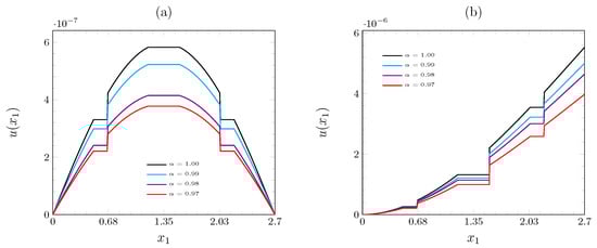
Figure 3.
Lateral displacement in the form of a devil’s staircase on Carpinteri’s beams: (a) simply supported beam, and (b) cantilever beam.
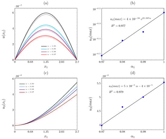
Figure 4.
Lateral displacement on Balankin’s beams for the fractal Timoshenko beam theory: (a) simply supported beam, where the dotted lines represent the displacement using the fractal Euler–Bernoulli equation, (b) maximum displacement of the simply supported beam as a function of , (c) cantilever beam, where the dotted lines represent the displacement using the fractal Euler–Bernoulli equation), and (d) maximum displacement of the cantilever beam as a function of .
Discussion of Results
The mechanical behavior of Carpinteri’s and Balankin’s beams has been analyzed from the perspective of the Timoshenko beam theory and for different Hausdorff dimensions: and . The geometries of the beams are given in Table 1.
The deflection curve has been calculated for two cases: the simply supported beam subjected to a uniformly distributed load and the cantilever beam subjected to a concentrated load applied at its free end, as illustrated in Figure 2. In the case of Carpinteri’s beam, the deflection curves for the second iteration are shown in Figure 3a, where it can be observed that under the same loading conditions as in a simply supported beam, the deflection increases with the value of . For the value of , the maximum deflection is obtained, whereas for , the minimum deflection curve is obtained. We can say that the stiffness of the bending increases as the value of decreases.
Similarly, in the case of the cantilever beam in Figure 3b, it can be seen that the flexural stiffness of the beam increases as the value of increases for the same load conditions. In addition, a stepped deformation behavior in the form of a devil’s staircase can be observed in this type of beam, assuming that the beam has no deflection in each step.
Figure 4a shows the deflection for the simply supported condition of Balankin’s beam subjected to a uniformly distributed load for various Hausdorff dimensions: , and . It can be observed that the maximum deflection is obtained with values of , corresponding to a classical Timoshenko beam. In the same figure, the deflection curve of the Euler–Bernoulli beam is shown with dotted lines. It can be seen that the Euler–Bernoulli beam has a shorter deflection compared to the Timoshenko beam. Figure 4b shows the trend of the maximum deflection value in relation to the Hausdorff dimension . The maximum deflection exhibits an exponential relationship with .
Figure 4c shows Balankin’s cantilever beam. As in the previous case, the beam exhibits a larger deflection for higher values of , with the curve showing the largest deflection when . For the cantilever beam, it has been found that there is a linear relationship between the maximum deflection and the Hausdorff dimension .
Finally, comparisons between the standard and fractal cases are shown in Figure 5, for and .
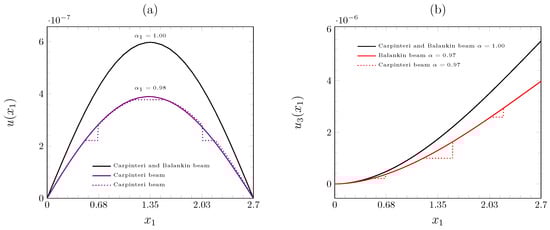
Figure 5.
Lateral displacement of Carpinteri’s and Balankin’s beams: (a) simply supported beam, and (b) cantilever beam.
5. Conclusions
In this work, a specific set of differential operators in the fractal continuum framework was used to describe the structural response of complex scale-invariant beams. These beams are impossible to model using conventional vector differential calculus due to the irregular functions defined on fractal domains, which are non-differentiable in the conventional sense. So, a generalization of the Timoshenko beam theory was conducted, transitioning from ordinary to fractal calculus.
The proposed formulation was applied to fractal beams with two different boundary conditions to validate it and describe the effects of fractal parameters in beams with complex domains. From this study, the following conclusions and outlooks can be drawn:
- i
- The stiffness of the self-similar beam is governed by the parameters , , , and the iteration number of the pre-fractal.
- ii
- The flexural rigidity is affected by the geometry and fractal topology of the beam, such that when increases, decreases. However, Carpinteri’s beam is stiffer than Balankin’s beam, as shown in Figure 4a,c.
- iii
- The fractal mass of each iteration and the boundary conditions of beams, as well as the length scales of similarity, are linked with the scale effect of fractal beams.
- iv
- Using the generalized Timoshenko beam formulation is possible to obtain the exact solutions of a complex scale-invariant beam through the parameter , which includes its topology and fractal geometry.
- v
- The introduced solution coincides with the classical Timoshenko beam theory when .
- vi
- A devil’s staircase-like structural response is presented in Carpinteri’s beams.
- vii
- In future work, we will extend this formulation to model self-similar column buckling. It is also possible to understand the mechanical behavior of other fractal beams, for example, Koch’s curve-like beam suggested in [49,50,51].
Author Contributions
Writing—original draft preparation, D.S.; Writing—review and editing, F.J.B.-L. and H.M.; Conceptualization, C.R.T.-S. and A.A.; Methodology, H.M. and F.J.B.-L.; Software, A.A.; Formal analysis, D.S. and C.R.T.-S.; Visualization, A.A. and F.J.B.-L.; Supervision, D.S. and H.M. All authors have read and agreed to the published version of the manuscript.
Funding
This work was supported by the Instituto Politécnico Nacional under the research SIP-IPN grant numbers 20230048, 20231176, and 20231131.
Data Availability Statement
Not applicable.
Conflicts of Interest
The authors declare no conflict of interest.
References
- Carpinteri, A.; Cornetti, P.; Sapora, A. A fractional calculus approach to nonlocal elasticity. Eur. Phys. J. Spec. Top. 2011, 193, 193–204. [Google Scholar] [CrossRef]
- Di-Paola, M.; Zingales, M. Long-range cohesive interactions of non-local continuum faced by fractional calculus. Int. J. Solids Struct. 2008, 45, 5642–5659. [Google Scholar] [CrossRef]
- Drapaca, C.S.; Sivaloganathan, S. A Fractional Model of Continuum Mechanics. J. Elast. 2012, 107, 105–123. [Google Scholar] [CrossRef]
- Sumelka, W. Thermoelasticity in the Framework of the Fractional Continuum Mechanics. J. Therm. Stress. 2014, 37, 678–706. [Google Scholar] [CrossRef]
- Lazopoulos, K.A. On Λ-Fractional Analysis and Mechanics. Axioms 2022, 11, 85. [Google Scholar] [CrossRef]
- Zubair, M.; Mughal, M.J.; Naqvi, Q.A. Electromagnetic Fields and Waves in Fractional Dimensional Space; Springer Science & Business Media: Berlin/Heidelberg, Germany, 2012. [Google Scholar]
- Balankin, A.S. Stresses and strains in a deformable fractal medium and in its fractal continuum model. Phys. Lett. 2013, 377, 2535–2541. [Google Scholar] [CrossRef]
- Parvate, A.; Satin, S.; Gangal, A.D. Calculus on fractal curves in Rn. Fractals 2011, 19, 15–27. [Google Scholar] [CrossRef]
- Tarasov, V.E. Continuous medium model for fractal media. Phys. Lett. 2005, 336, 167–174. [Google Scholar] [CrossRef]
- Li, J.; Ostoja-Starzewski, M. Fractal solids, product measures and fractional wave equations. Proc. R. Soc. A 2009, 465, 2521–2536. [Google Scholar] [CrossRef]
- Golmankhaneh, A.K. Fractal Calculus and Its Applications: Fα-Calculus; World Scientific: Singapore, 2022. [Google Scholar]
- Falconer, K. Techniques in Fractal Geometry; John Wiley and Sons: Hoboken, NJ, USA, 1997. [Google Scholar]
- Falconer, K. Fractal Geometry-Mathematical Foundations and Applications, 3rd ed.; Wiley: Hoboken, NJ, USA, 2014. [Google Scholar]
- Kigami, J. Analysis on Fractals; Cambridge University Press: Cambridge, UK, 2000. [Google Scholar]
- Mandelbrot, B.B. Fractals: Form, Chance and Dimension; Echo Point Books & Media: Brattleboro, VT, USA, 2020. [Google Scholar]
- Davey, K.; Rasgado, A. Analytical solutions for vibrating fractal composite rods and beams. Appl. Math. Model. 2011, 35, 1194–1209. [Google Scholar] [CrossRef]
- Rostami, H.; Najafabadi, M.; Ganji, D. Analysis of Timoshenko beam with Koch snowflake cross-section and variable properties in different boundary conditions using finite element method. Adv. Mech. Eng. 2021, 13, 16878140211060982. [Google Scholar] [CrossRef]
- Samayoa, D.; Mollinedo, H.; Jiménez-Bernal, J.A.; Gutiérrez-Torres, C.d.C. Effects of Hausdorff Dimension on the Static and Free Vibration Response of Beams with Koch Snowflake-like Cross Section. Fractal Fract. 2023, 7, 153. [Google Scholar] [CrossRef]
- Stempin, P.; Sumelka, W. Space-fractional Euler-Bernoulli beam model - Theory and identification for silver nanobeam bending. Int. J. Mech. Sci. 2020, 186, 105902. [Google Scholar] [CrossRef]
- Lazopoulos, K.A.; Lazopoulos, A.K. On fractional bending of beams with A-fractional derivative. Arch. Appl. Mech. 2020, 90, 573–584. [Google Scholar] [CrossRef]
- Blaszczyk, T.; Siedlecki, J.; Sun, H.G. An exact solution of fractional Euler-Bernoulli equation for a beam with fixed-supported and fixed-free ends. Appl. Math. Comput. 2021, 396, 125932. [Google Scholar] [CrossRef]
- Yang, A.; Zhang, Q.; Qu, J.; Cui, Y.; Chen, Y. Solving and Numerical Simulations of Fractional-Order Governing Equation for Micro-Beams. Fractal Fract. 2023, 7, 204. [Google Scholar] [CrossRef]
- Lazopoulos, K.A. Stability Criteria and Λ-Fractional Mechanics. Fractal Fract. 2023, 7, 248. [Google Scholar] [CrossRef]
- Ostoja-Starzewski, M.; Li, J. Fractal materials, beams, and fracture mechanics. Z. Angew. Math. Phys. 2009, 60, 1194–1205. [Google Scholar] [CrossRef]
- Samayoa, D.; Damián-Adame, L.; Kryvko, A. Map of a Bending Problem for Self-Similar Beams into the Fractal Continuum Using the Euler–Bernoulli Principle. Fractal Fract. 2022, 6, 230. [Google Scholar] [CrossRef]
- Samayoa, D.; Kryvko, A.; Velázquez, G.; Mollinedo, H. Fractal Continuum Calculus of Functions on Euler-Bernoulli Beam. Fractal Fract. 2022, 6, 552. [Google Scholar] [CrossRef]
- Golmankhaneh, A.K.; Ali, K.K.; Yilmazer, R.; Awad Kaabar, M.K. Local fractal Fourier transform and applications. Comput. Methods Differ. Equ. 2022, 10, 595–607. [Google Scholar] [CrossRef]
- Carpinteri, A.; Chiaia, B.; Cornetti, P. A fractal theory for the mechanics of elastic materials. Mater. Sci. Eng. 2004, 365, 235–240. [Google Scholar] [CrossRef]
- Carpinteri, A.; Chiaia, B.; Cornetti, P. A disordered microstructure material model based on fractal geometry and fractional calculus. ZAMM Appl. Math. Mech. 2004, 84, 128–135. [Google Scholar] [CrossRef]
- Carpinteri, A.; Corneti, P.; Sapora, A.; Di Paola, M.; Zingales, M. Fractional calculus in solid mechanics: Local versus non-local approach. Phys. Scr. 2009, 2009, 014003. [Google Scholar] [CrossRef]
- Carpinteri, A.; Sapora, A. Diffusion problems in fractal media defined on Cantor sets. ZAMM Angew. Math. Mech. 2010, 90, 203–210. [Google Scholar] [CrossRef]
- Li, J.; Ostoja-Starzewski, M. Micropolar continuum mechanics of fractal media. Int. J. Eng. Sci. 2011, 249, 1302–1310. [Google Scholar] [CrossRef]
- Joumaa, H.; Ostoja-Starzewski, M. Elastodynamics in micropolar fractal solids. Math. Mech. Solids 2014, 19, 117134. [Google Scholar] [CrossRef]
- Balankin, A.S. A continuum framework for mechanics of fractal materials I: From fractional space to continuum with fractal metric. Eur. J. Phys. 2015, 88, 90. [Google Scholar] [CrossRef]
- Balankin, A.S.; Elizarraraz, B.E. Map of fluid flow in fractal porous medium into fractal continuum flow. Phys. Rev. 2012, 85, 056314. [Google Scholar] [CrossRef]
- Balankin, A.S.; Elizarraraz, B.E. Reply to “Comment on ‘Hydrodynamics of fractal continuum flow’ and ‘Map of fluid flow in fractal porous medium into fractal continuum flow’”. Phys. Rev. 2013, 88, 057002. [Google Scholar] [CrossRef]
- Tarasov, V.E. Vector calculus in non-integer dimensional space and its applications to fractal media. Commun. Nonlinear Sci. Numer. Simul. 2015, 20, 360–374. [Google Scholar] [CrossRef]
- Li, J.; Ostoja-Starzewski, M. Micropolar mechanics of product fractal media. Proc. R. Soc. A 2022, 478, 20210770. [Google Scholar] [CrossRef]
- El-Nabulsi, R.A. On nonlocal fractal laminar steady and unsteady flows. Acta Mech. 2021, 232, 1413–1424. [Google Scholar] [CrossRef]
- Balankin, A.S.; Elizarraraz, B.E. Hydrodynamics of fractal continuum flow. Phys. Rev. 2012, 85, 025302(R). [Google Scholar] [CrossRef]
- Anukool, W.; El-Nabulsi, R.A. Fractal dimension modeling of seismology and earthquakes dynamics. Acta Mech. 2022, 233, 2107–2122. [Google Scholar] [CrossRef]
- El-Nabulsi, R.A.; Golmankhane, A.K. Propagation of waves in fractal spaces. Waves Random Complex Media 2023, 1–23. [Google Scholar] [CrossRef]
- Mashayekhi, S.; Miles, P.; Yousuff-Hussaini, M.; Oates, W.S. Fractional viscoelasticity in fractal and non-fractal media: Theory, experimental validation, and uncertainty analysis. J. Mech. Phys. Solids 2018, 111, 134–156. [Google Scholar] [CrossRef]
- Balankin, A.S. A continuum framework for mechanics of fractal materials II: Elastic stress fields ahead of cracks in a fractal medium. Eur. J. Phys. 2015, 88, 91. [Google Scholar] [CrossRef]
- Hall, P.; Wood, A. On the performance of box-counting estimators of fractal dimension. Biometrika 1993, 80, 246–251. [Google Scholar] [CrossRef]
- Chun-Hui, H.; Chao, L. Fractal dimensions of a porous concrete and its effect on the concrete’s strength. Fracta Univ. 2023, 21, 137–150. [Google Scholar] [CrossRef]
- Balankin, A.S.; Mena, B. Vector differential operators in a fractional dimensional space, on fractals, and in fractal continua. Chaos Solitons Fractals 2023, 168, 113203. [Google Scholar] [CrossRef]
- Balankin, A.S.; Ramírez-Joachim, J.; González-López, G.; Gutiérrez-Hernández, S. Formation factors for a class of deterministic models of pre-fractal pore-fracture networks. Chaos Solitons Fractals 2022, 162, 112452. [Google Scholar] [CrossRef]
- Carpinteri, A.; Pugno, N.; Sapora, A. Asymptotic analysis of a von Koch beam. Chaos Solitons Fractals 2009, 41, 795–802. [Google Scholar] [CrossRef]
- Carpinteri, A.; Pugno, N.; Sapora, A. Free vibration analysis of a von Koch beam. Int. J. Solids Struct. 2010, 47, 1555–1562. [Google Scholar] [CrossRef]
- Carpinteri, A.; Pugno, N.; Sapora, A. Dynamic response of damped von Koch antennas. J. Vib. Control. 2010, 17, 733–740. [Google Scholar] [CrossRef]
Disclaimer/Publisher’s Note: The statements, opinions and data contained in all publications are solely those of the individual author(s) and contributor(s) and not of MDPI and/or the editor(s). MDPI and/or the editor(s) disclaim responsibility for any injury to people or property resulting from any ideas, methods, instructions or products referred to in the content. |
© 2023 by the authors. Licensee MDPI, Basel, Switzerland. This article is an open access article distributed under the terms and conditions of the Creative Commons Attribution (CC BY) license (https://creativecommons.org/licenses/by/4.0/).