Article

On the Fundamental Diagram for Freeway Traffic: Exploring the Lower Bound of the Fitting Error and Correcting the Generalized Linear Regression Models

1
Department of Logistics and Maritime Studies, Faculty of Business, The Hong Kong Polytechnic University, Hung Hom, Hong Kong
2
College of Civil Engineering and Architecture, Zhejiang University, Hangzhou 310058, China
3
Department of Architecture and Civil Engineering, Chalmers University of Technology, 412 96 Göteborg, Sweden
4
State Key Laboratory of Mechanical Transmission/Automotive Collaborative Innovation Center, Chongqing University, Chongqing 400044, China
5
Department of Building and Real Estate, The Hong Kong Polytechnic University, Hung Hom, Hong Kong
*
Author to whom correspondence should be addressed.
Mathematics 2023, 11(16), 3460; https://doi.org/10.3390/math11163460
Submission received: 4 July 2023 / Revised: 25 July 2023 / Accepted: 8 August 2023 / Published: 9 August 2023
(This article belongs to the Special Issue Applied Mathematics in Supply Chain and Logistics)

Abstract

:
In traffic flow, the relationship between speed and density exhibits decreasing monotonicity and continuity, which is characterized by various models such as the Greenshields and Greenberg models. However, some existing models, i.e., the Underwood and Northwestern models, introduce bias by incorrectly utilizing linear regression for parameter calibration. Furthermore, the lower bound of the fitting errors for all these models remains unknown. To address above issues, this study first proves the bias associated with using linear regression in handling the Underwood and Northwestern models and corrects it, resulting in a significantly lower mean squared error (MSE). Second, a quadratic programming model is developed to obtain the lower bound of the MSE for these existing models. The relative gaps between the MSEs of existing models and the lower bound indicate that the existing models still have a lot of potential for improvement.

1. Introduction

The traffic fundamental diagram is crucial in traffic flow theory [1,2,3,4,5], representing the relationship between traffic flow (vehs/h), speed (km/h), and traffic density (vehs/km). Greenshields [1] first proposed a linear model to describe the relationship between speed and density and made a pioneering work in this field. This rudimentary relationship has since been refined through the introduction of numerous models [3,4,5,6,7,8,9,10,11,12,13,14,15,16,17,18]. These studies try to define precise relationships, utilizing practical parameters to reflect the traffic flow features more accurately. This paper focuses on the four well-known models listed in Table 1, each having two parameters.
At the same time, a great number of calibration models have been proposed related to these well-known models. Qu et al. [19] proposed a least-squares method to calibrate the model so that the model can be applied to both in light-traffic/free-flow conditions and congested/jam conditions. Fan and Seibold [21] and Qu et al. [22] published research works using data-driven approaches to generate a percentile-based speed–density relation-ships for freeway traffic. Wang [23] addressed the shortcomings of data-driven stochastic fundamental maps of diagram traffic by proposing a holistic modelling framework based on the concept of mean absolute error minimization. For more related literature, please refer to Bramich et al. [24]. Nearly all existing studies employ linear regression to solve these famous models and estimate parameters [25,26,27,28]. For models that cannot be solved directly by linear regression, such as the Underwood and Northwestern models, many researchers resort to defining y = l n v and x = k for the Underwood model and y = l n v and x = k 2 for the Northwestern model to transform them into linear models of x , y , whose parameters can be easily estimated by linear regression. However, this transformation is fundamentally flawed, as it fails to obtain an unbiased estimate of v . The problem arises from the fact that the estimate of parameter l n v cannot accurately represent the estimate of parameter v , leading to a distorted and biased final estimate. Given this challenge, this study aims to address this issue.
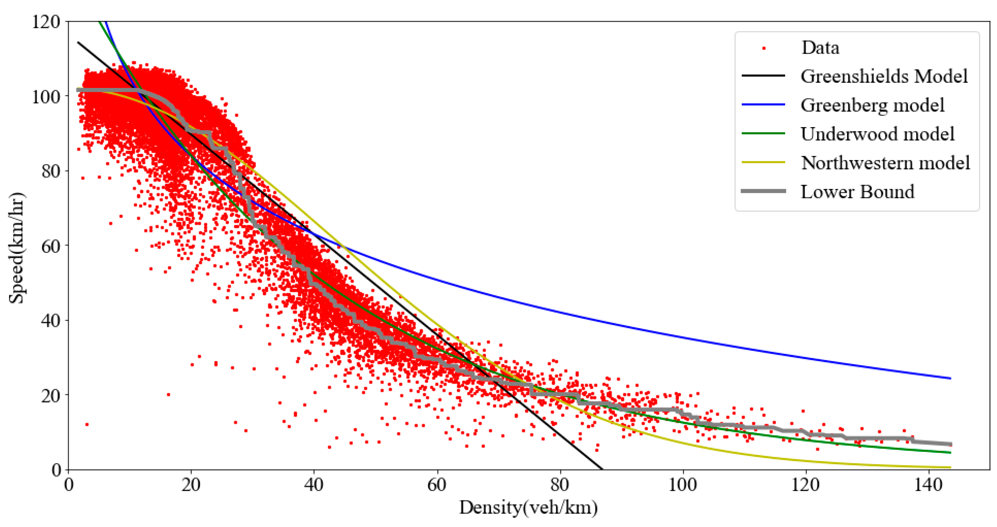
In the calibration and validation of traffic flow fundamental diagrams, numerous studies use a specific dataset [13,19,22,23,29,30], which makes our comparison more consistent, as shown in Figure 1. This dataset comprises 47,815 speed-density observations collected over a year by loop detectors from 76 stations on Georgia State Route 400 (hereafter referred to as the GA400 dataset). The GA400 dataset facilitates the examination of the performance of the four models, as shown in Figure 1. Each of the four models has its own strengths when describing the characteristics of the speed and density relationship: for example, the Greenshields and Northwestern models perform better in low-density datasets, while the Underwood model performs better in medium- to high-density datasets. Despite the widespread application of the four models, a key issue—the gap between their fittings and the “ideal” lower bound of the fitting error—remains unanswered in the existing literature. To address this research gap, this paper defines the model that minimizes the MSE of the dataset among all monotonically decreasing models as an “ideal” prediction model whose optimal objective function value is thus termed the lower bound of the fitting error.
The main contributions of this paper are twofold. We first show that applying the transformation on the Underwood and Northwestern models produces biased results. In response to this finding, we correct the methodological errors involved in using linear regression for parameter estimation in these models. Second, we construct a quadratic programming model with the objective of minimizing the MSE to find the “ideal” lower bound of the fitting error for existing models. The results show that the average relative gap between the lower bound and the MSEs of existing models is about 197.322%. Therefore, there is still a lot of room for further development of existing models.
The rest of the paper is organized as follows. In Section 2, we prove that using linear regression to calibrate nonlinear relationships between k and v is biased and then correct this error using the enumeration approach. Section 3 establishes a quadratic programming model to find the “ideal” lower bound of the fitting error of existing models. Section 4 concludes this study.

2. Correcting Generalized Linear Regression Models

2.1. Analysis

In the existing studies, the parameters v f and k 0 of Underwood and Northwestern models are estimated by linear regression. The procedures are as follows.
In the Underwood model, v = v f e x p 1 k k 0 , and the parameters to be estimated are v f and k 0 . By taking the logarithm on both sides of the equation, the model is equivalent to l n v l n v f = k k 0 . After letting y = l n v and x = k , the model is transformed into y = l n v f x k 0 . By performing a linear regression on x and y , we obtain the equation y = a x + b , where a and b are the parameters derived from the regression. Consequently, the parameters v f and k 0 can be estimated as v f = e x p ( b ) and k 0 = 1 a .
In the Northwestern model, v = v f e x p 1 2 k k 0 2 , and the parameters to be estimated are v f and k 0 . By taking the logarithm on both sides of the equation, the model is equivalent to l n v = l n v f 1 2 k k 0 2 . After letting y = l n v and x = k 2 , the model is transformed into y = l n v f 1 2 x k 0 2 . By performing a linear regression on x and y , we obtain the equation y = c x + d , where c and d are the parameters derived from the regression. Consequently, the parameters v f and k 0 can be estimated as v f = e x p ( d ) and k 0 = 1 2 c .
The above procedures use the logarithm of v and then apply linear regression. In order to correctly use linear regression to estimate the parameters of the models, we should guarantee that the unbiased estimate of v is equivalent to the exponential of the unbiased estimate of y . However, this condition may not be satisfied in some cases. For example, assume v has three realizations: 3, 4, and 5. The unbiased estimate of the expectation of v is 4 (the sample mean); however, e x p l n 3 + l n 4 + l n 5 3 3.915 is not the original unbiased estimate of the expectation of v . Therefore, the exponential of the unbiased estimate of l n v results in a biased estimate of v . In the following, we discuss the unbiased and biased estimation cases under transformation.
Lemma 1.
If the transformed samples used for linear regression are strictly linearly correlated, the estimates of parameters are unbiased.
Proof. 
Using the least-squares method for linear regression, y ^ i = a x i + b   ( i { 1 , , n } , where n is the number of data samples, we minimize the sum of squares of the errors  R S S S S E , which can be expressed as given:
R S S S S E = i = 1 n ( y i y ^ i ) 2 = i = 1 n [ y i ( a x i + b ) ] 2 .
Solving the above equation by means of derivatives, we can obtain the following:
b = y ¯ a x ¯ ,
a = i = 1 n x i x ¯ ( y i y ¯ ) i = 1 n x i x ¯ 2 ,
where x ¯ = 1 n i = 1 n x i , and y ¯ = 1 n i = 1 n y i .
When solving the Underwood model using linear regression, let y = l n v and  x = k , and we can obtain the following:
v ^ i = exp y ^ i = exp a ^ x i + b ^ = exp a ^ x i + y ¯ a ^ x ¯ = exp a ^ x ¯ + b ^ + a ^ x i x ¯ = e x p a ^ x i + b ^ .
If all points x i , y i are co-linear, then
v ^ i = exp a ^ x i + b ^ = e x p ( y ^ i ) = e x p y i .
Therefore, the estimates of the linear regression after transmission are unbiased; namely, we have the following:
E v ^ = v ¯
where  v ^ is the estimated v , and v ¯ = 1 n i = 1 n v i . □
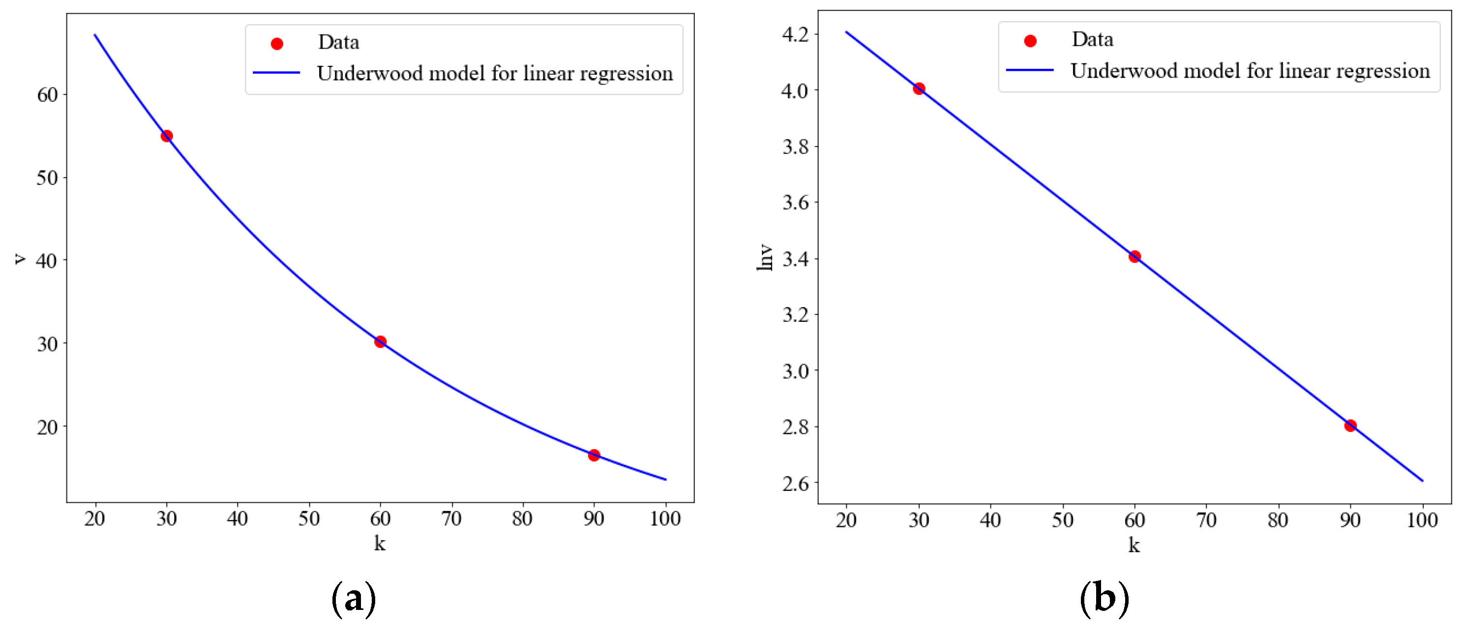
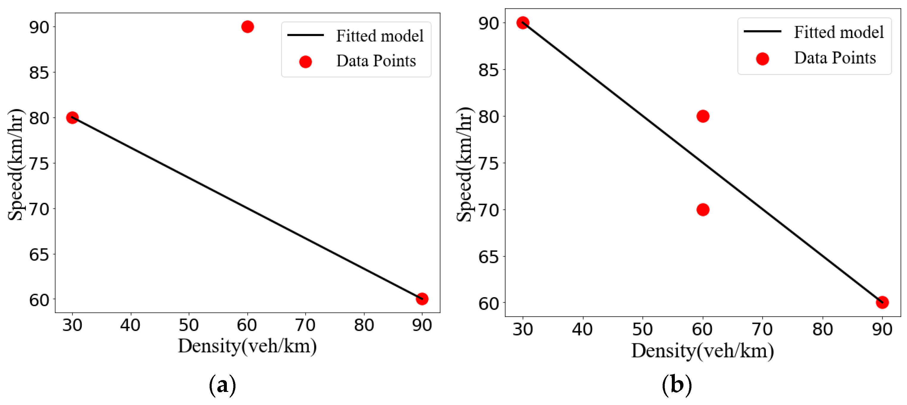
Taking the Underwood model as an example, suppose there are three given points of k , v , which are (30, 54.881), (60, 30.119), and (90, 16.530), as shown in Figure 2a. Let y = l n v and x = k ; the three points are transformed to (30, 4.005), (60, 3.405), and (90, 2.805). Obviously, these three points can be linked by a straight line, as shown in Figure 2b. Performing a linear regression on k , l n v , we obtain the fitted linear expression y = 4.6052 + ( 0.02 ) x . We use the MSE to express the fitting error, which is the cumulative value of the differences between actual observations and predicted values. The MSE can be computed as follows:
M S E = 1 n i = 1 n v i v ^ i 2  
where v ^ i is the value predicted by the model, v i is the real value, and n is the number of observations in the dataset. Thus, the MSE of the fitted line to the transformed samples is zero.
Transforming the parameters from the linear regression back into the original model, we obtain v f = e x p ( 4.6052 ) and k 0 = 1 0.02 . The original Underwood model should be v = e x p 4.6052 + 0.02 k , and the MSE of the fitted exponential curve to the original samples is also zero. Consequently, the density k and speed v of these samples obey the exponential relationship and strictly adhere to the Underwood model, as illustrated in Figure 2a.
However, when the data points used for linear regression do not lie on a straight line, the linear fitting is meaningless, and the estimates are biased. Therefore, we give the case where the linear transformation presents a bias against the Underwood and Northwestern models.
Lemma 2.
If the transformed samples used for linear regression are not strictly linearly correlated, the estimates of the parameters are generally biased.
Proof. 
If we only have two points, they must be co-linear. We now discuss the case of three points. If the estimate is biased when the transformed three points are not co-linear, then the estimate must also be biased when more transformed points are not co-linear. Consider the three points x 1 , y 1 , x 2 , y 2 , a n d x 3 , y 3  in the dataset that are not co-linear. If there are two points with equal y  values, the x  values are different. However, it is not possible for the y  values of the three points to be equal since they would be co-linear. Hence, the relationship between the y  values of these three points can be expressed as given: y 1 < y 2 < y 3  or y 1 y 2 < y 3  or y 1 < y 2 y 3 . We define the following:
v ¯ = v 1 + v 2 + v 3 = exp y 1 + exp y 2 + exp y 3 .
Let y ^ i = y i + i ( i = 1 , 2 , 3 ) ; then, we define the following:
E v ^ : = exp y 1 + 1 + exp y 2 + 2 + exp y 3 + 3 .
Therefore, we have the following:
E v ^ v ¯ = y 1 y 1 + 1 exp x d x + y 2 y 2 + 2 exp x d x + y 3 y 3 + 3 exp x d x .
Meanwhile, in linear regression, the estimated y is unbiased; namely, we obtain E ( y ^ ) = y ¯ , and 1 n i = 1 n y ^ i = 1 n i = 1 n ( y i + i ) = 1 n i = 1 n y i . Thus, 1 + 2 + 3 = 0 . Therefore, we obtain the following:
v ^ v ¯ = y 1 y 1 + 1 exp x d x + y 2 y 2 + 2 exp x d x + y 3 y 3 1 2 exp x d x .
In exp x , all the different ranges of x values correspond to different function values. Therefore, to guarantee the estimates are unbiased, E v ^ v ¯ = 0 should be satisfied. To meet E v ^ = v ¯ , we need y 1 + 1 = y 2  and y 3 1 2 = y 1 ; namely, y ^ 1 = y 2 , and y ^ 3 = y 1 . Obviously, this situation does not exist. Thus, in the transformed dataset, the solution using linear programming is biased as long as the three points are not co-linear. □
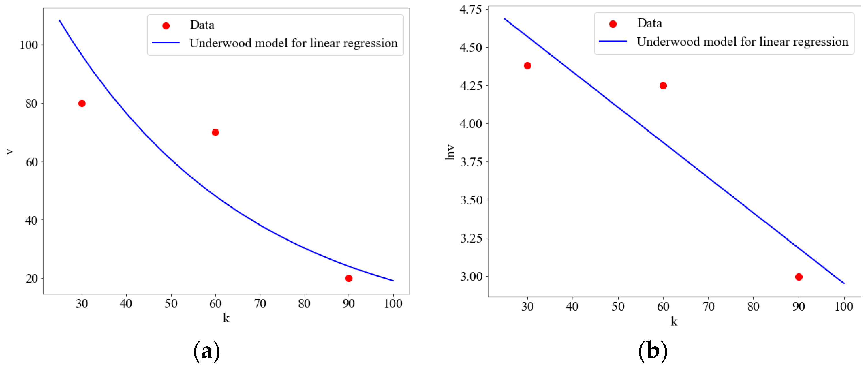
Taking the Underwood model as an example, suppose there are three given points of k , v , which are (30, 80), (60,70), and (90,20), as shown in Figure 3a. Let y = l n v and x = k ; the three points are transformed to (30, 4.382), (60, 4.249), and (90, 2.996). Clearly, these three points are not collinear, as shown in Figure 3b. Performing a linear regression on k , l n v , we obtain the fitted linear expression y = 5.2617 + ( 0.023105 ) x , whose MSE is 0.069593. However, when transforming the parameters from the linear regression back into the original model, v f = exp 5.2617 , and k 0 = 1 0.023105 , and the original Underwood model should be v = e x p 5.2617 + 0.023105 k , whose MSE is 253.6947. Because the transformed samples used for linear regression is not on the fitted line, it is meaningless to use linear regression to estimate the parameters of the model. Therefore, the fitted results obtained from the linear regression are not the true picture of the model, and the estimates of the model are biased.
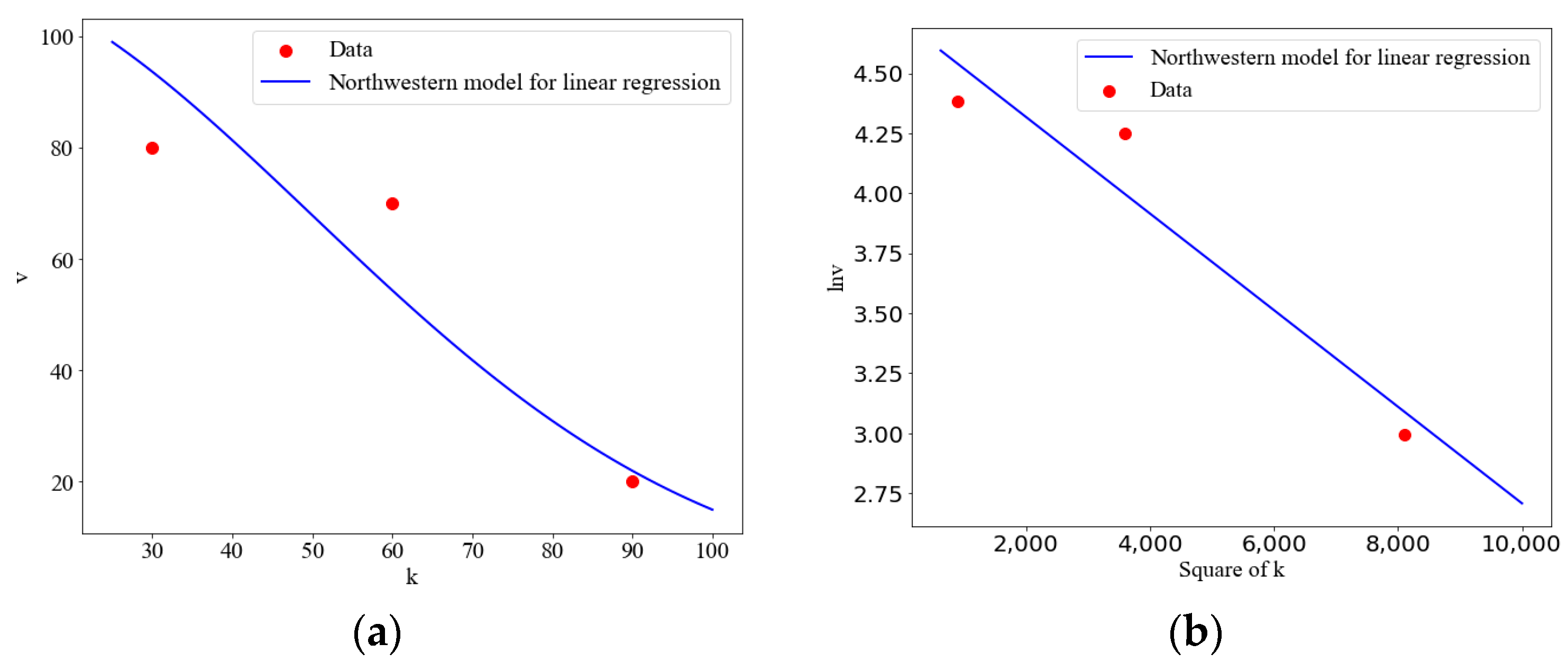
Taking the example in the Underwood model, suppose the three given points of coincide with the above example, as in Figure 4a. Let y = l n v and x = k 2 ; the three points are transformed to (900, 4.382), (3600, 4.248), and (8100, 2.996). Obviously, these points are also not collinear, as in Figure 4b. Performing a linear regression on k 2 , l n v gives results with an MSE of 0.03248981, and the fitted linear expression is y = 4.7209 + ( 0.0002013 ) x . However, when substituting the parameters from the linear regression back into the original model, we obtain v f = e x p ( 4.7209 ) and k 0 = 1 2 × ( 0.0002013 ) , and the original Underwood model should be v = e x p 4.7209 0.0002013 k 2 , whose MSE is 144.75979. Although the MSE value of the linear regression is good, this advantage cannot be reflected in the original model because the points used for linear regression are not collinear (as shown in Figure 4a). As a result, the linear regression approach is biased.
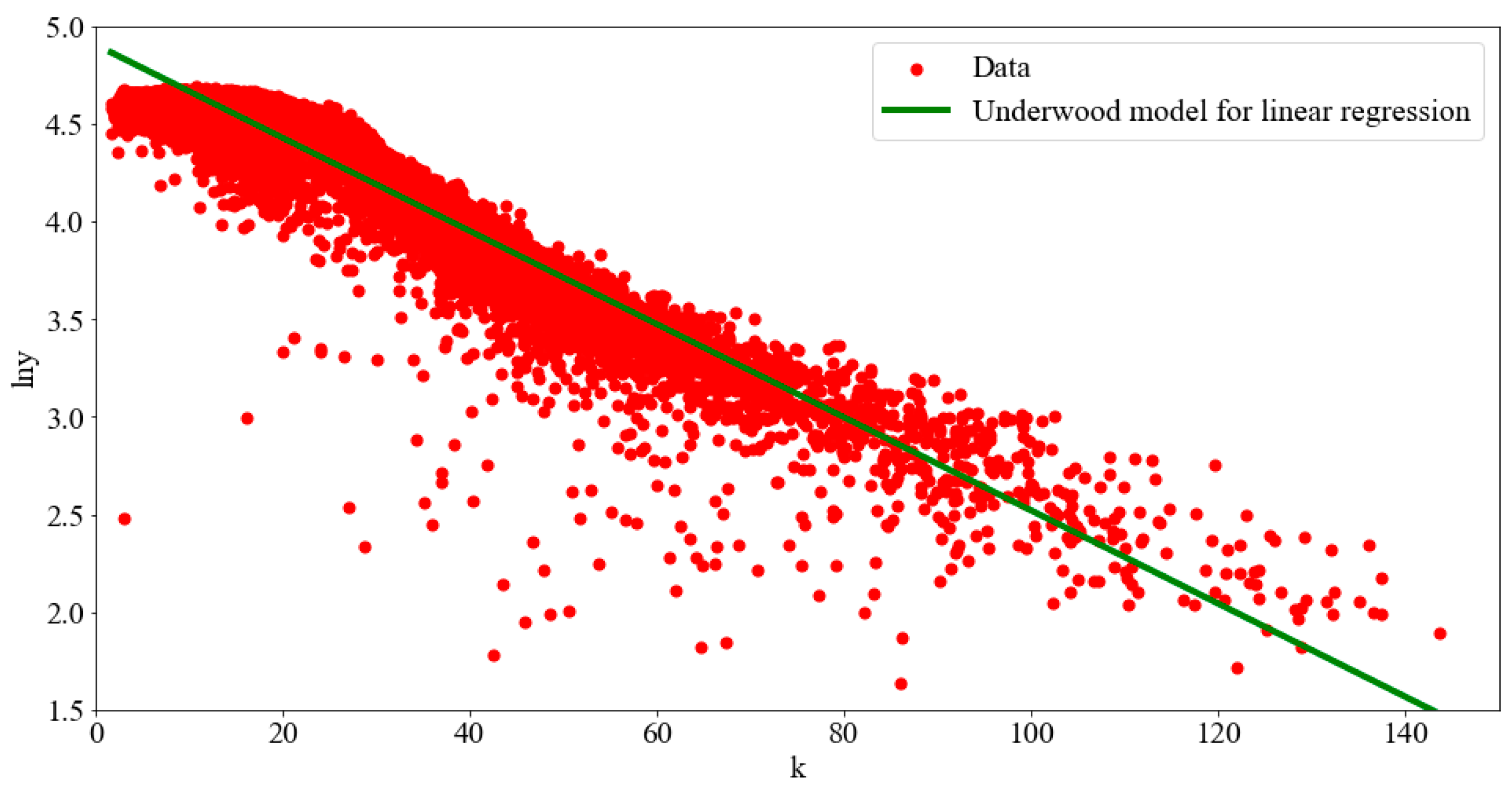
Figure 5 and Figure 6 depict the samples after the transformation of GA400 for the Underwood and Northwestern models. It is evident that these simple, straight lines in Figure 5 and Figure 6 cannot fully capture the underlying structure of these points. Consequently, these two linear regression models provide biased estimates in this context.

2.2. Correction

For the case where the linear regression provides biased estimates, we re-solve the model parameters using an enumeration algorithm. That is, we try to find the parameter values corresponding to the smallest MSE within the feasible ranges of the parameters, as shown in Algorithm 1. The estimated parameters obtained are unbiased for a given precision, and better estimates may exist as the precision becomes smaller. The enumeration algorithm is universal for estimated parameters that are difficult to solve by approximation or derivation methods.
Algorithm 1: An enumeration algorithm.
Input: A set of candidate pairs of parameters v f i , k 0 j i = 1 , 2 , , M ; j = 1 , 2 , , N .
Output: The minimum MSE, the optimal values of parameters.
M S E v f i , k 0 j denotes the MSE value of the pair of parameters v f i , k 0 j ; the minimum MSE and its corresponding optimal parameters are denoted as M S E , v f , k 0 .
Initialize the M S E = , v f = 0 , k 0 = 0 .
For  i = 1 , 2 , , M do:
  For  j = 1 , 2 , , N do:
    Calculate the MSE value M S E v f i , k 0 j for the pair of parameters v f i , k 0 j .
    If  M S E v f i , k 0 j M S E do:
       v f = v f i ,
       k 0 = k 0 j ,
       M S E = M S E v f i , k 0 j .
    End if
  End for
End for
The examples in Lemma 2 are solved with the enumeration algorithm, as shown in Figure 7. For the Underwood and Northwestern models, we enumerate the two parameters v f and k 0 in functions v = v f e x p 1 k k 0 and v = v f e x p [ 1 2 k k 0 2 ] , both with a precision of 1 and a range of 0 to 200. The resulting optimal MSE values are 161.36348 and 93.4532, respectively. They are much better than the MSE values 253.6947 and 144.75979 obtained from the linear regression.
Above, we have corrected two simple examples using the enumeration algorithm, and next, we will examine how this algorithm performs on the entire GA400 dataset.
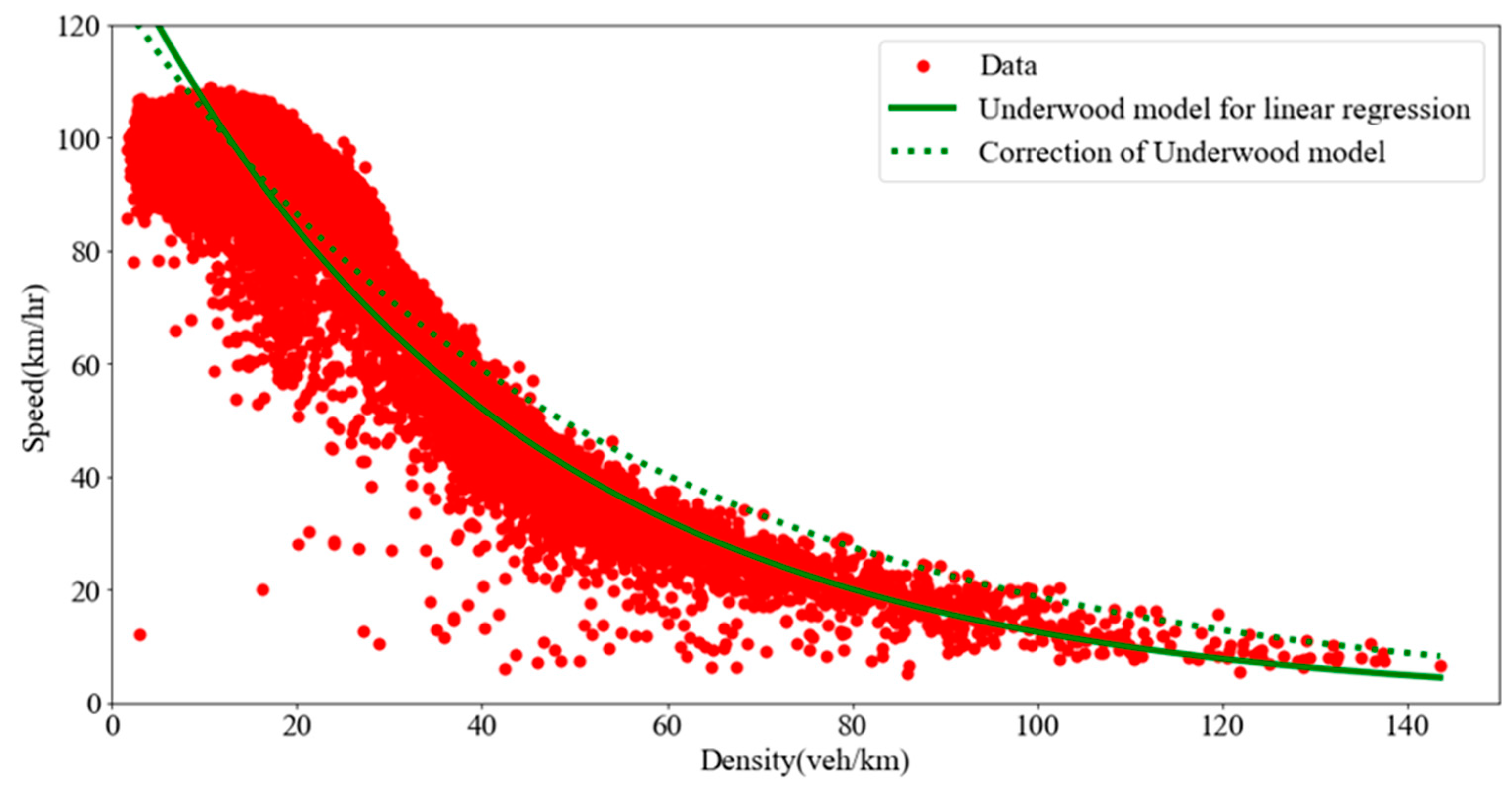
In the Underwood model, for parameters v f and k 0 , we set the iteration precision to 0.1 and the range to (0, 160) and (0, 120), respectively. The optimal values of parameters obtained are v f = 126.5790 and k 0 = 52.3435 , and the corresponding MSE is 50.36096, smaller than the MSE 59.4544 obtained from linear regression. Figure 8 illustrates the curves before and after the correction.
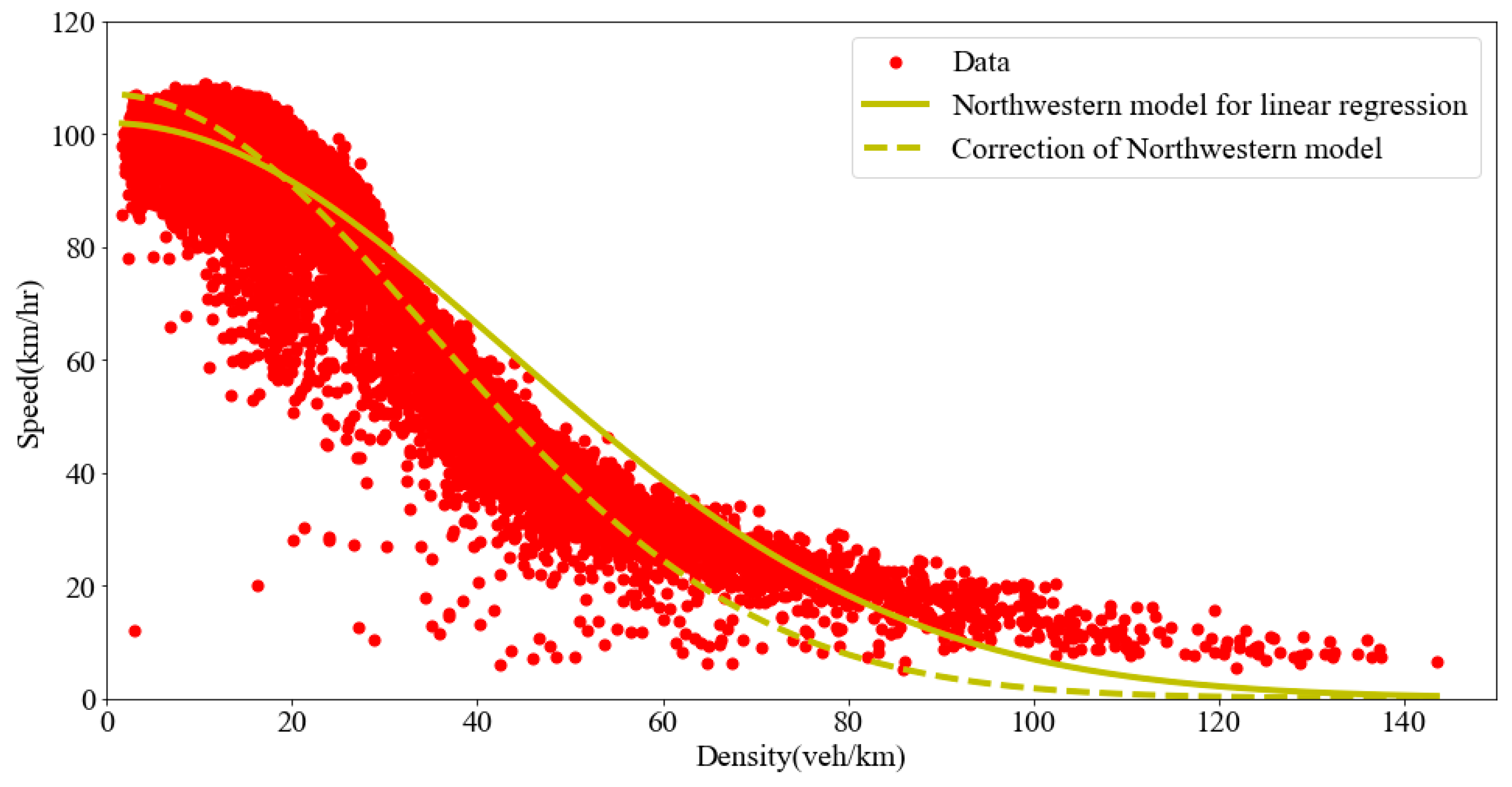
In the Northwestern model, for parameters v f and k 0 , we set the iteration precision to 0.1 and the range to (0, 160) and (0, 120), respectively. Then, we use the enumeration algorithm to find v f = 107.0668 and k 0 = 34.9348 . The MSE is 25.9371, much smaller than the MSE 44.3233 obtained from linear regression. The curves before and after correction are shown in Figure 9.
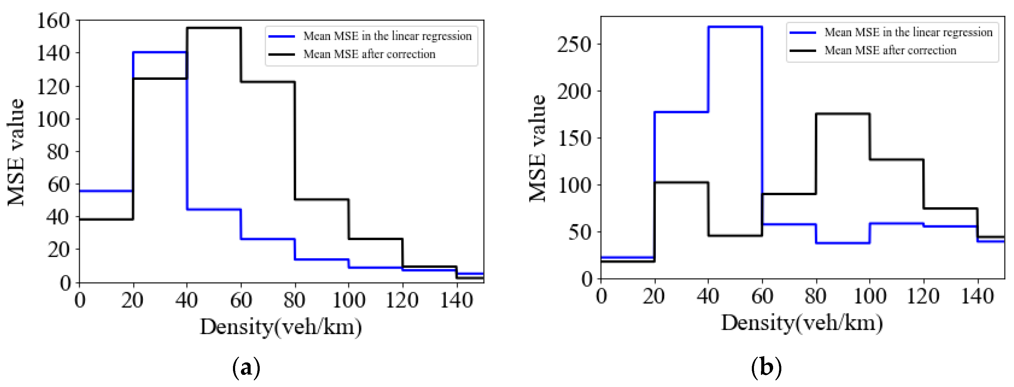
From Figure 8 and Figure 9, the corrected models appear to dominate only in the low-density range. This is because about 86% of the data points in the GA400 are concentrated in the [0, 20) range of the density. Figure 10a shows the average MSE value of the Underwood model for different density intervals, where the corrected results outperform the results solved by linear regression for densities in [0, 40) and [140, ∞), which account for 93% of all data points. Figure 10b shows the average MSE values of the Northwest model for different density intervals, and the corrected results are better than those solved by linear regression for densities [0, 60) and [140, ∞), which account for 98% of all data points. As a result, the features of a small portion of the data may be discarded in order to optimize the fit for the entire dataset.

3. Lower Bound of the Fitting Error of Existing Models

3.1. MSE Values of Existing Models

Table 2 illustrates the MSE values of the four models based on the GA400 dataset. Since linear regression is biased, the Underwood and Northwestern models make the differences in MSE values before and after the correction. The results show that the Northwestern model performs the best. Nevertheless, the MSE value of the Northwestern model is still high, motivating us to explore the lower bound of the fitting error for existing models.
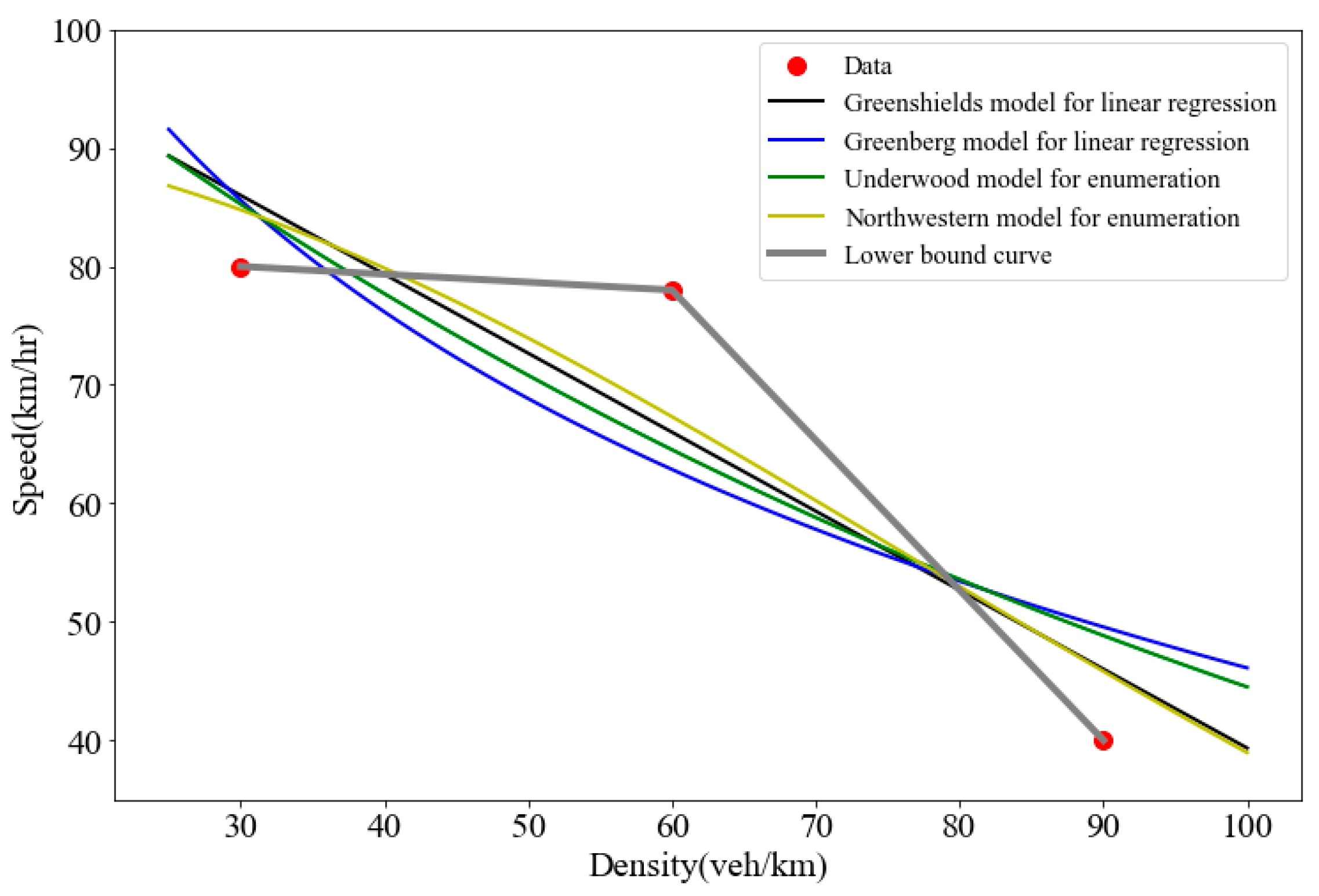
We use an example to illustrate how to compute the “ideal” lower bound of the fitting error. Given a dataset containing the three points (30,80), (60,78), and (90,40), Table 3 presents the MSEs for each of the four models, with the corresponding fitted curves displayed in Figure 11. Due to the models’ structure, none of them could be adjusted to achieve an MSE of zero, as evidenced by their inability to pass through all three points simultaneously. Consistent with the monotonicity and decreasing characters of the traffic flow, the speeds corresponding to each density value to achieve the minimum MSE are found and simply connected to form a piecewise linear function. This value is the lower bound of the model’s fitting error. Therefore, assessing the differences between the existing models’ MSEs and the lower bound exposes potential areas for improvement.

3.2. Quadratic Programming Model

Considering the monotonically decreasing and continuous characteristics of traffic flow, the prediction model, denoted by f k , with the minimum MSE should be selected among all possible monotonically decreasing continuous functions. This means that for two given densities, i.e., k 1 < k 2 , we should have f k 1 f k 2 and that for each density, there is only one speed output. We use the following two cases to illustrate this model.
Case 1: As shown in Figure 12a, actual speed may increase with increasing density, contrary to the general relationship where speed decreases as density increases. However, to capture the overall characteristic of traffic flow, any fitted model should exhibit both continuity and a monotonically decreasing trend. This allows the model to accommodate the unique cases while reflecting the general behavior of traffic flow.
Case 2: As shown in Figure 12b, different speeds can exist at the same density. However, the estimated speed in the model can only be a single value, which should ideally be the average of these speeds.
Considering these factors, we developed a quadratic programming model that defines the lower bound of the fitting error. The optimal objective function value of this model corresponds to the lower bound, providing a quantifiable measure of the fitting error. The model is shown as follows:
m i n 1 m i = 1 m v i j v ^ i 2
Subject to
v ^ i v ^ i + 1 0 ,   i = 1 , , m .
Here, v ^ i = f ( k i ) denotes the decision variable, representing the estimated speed at the i-th density f ( k i ) , and m is the number of all different densities. Considering that a same speed may correspond to multiple densities, we denote v i j as the j-th real speed value at the i-th density. Equation (2) is the objective function of the model that minimizes the MSE value. Constraint (3) requires that the estimated speeds should satisfy the characteristics of monotonically decreasing continuity in traffic flow.

3.3. Results

The above model capturing the lower bound of the fitting error can be viewed as a piece-wise linear function that links the optimal speed at each density. We utilize GUROBI to solve the model on the GA400 dataset, which achieves a minimum MSE of 19.360. This fitting error is significantly lower than the results obtained by the four models, as demonstrated in Figure 13. In the GA400 dataset, more than 80% of the data points are concentrated within the 0–20 density range. As a result, models tend to primarily focus on these points. However, our model optimizes the lower bound across all density intervals, making it applicable in all cases of density distribution. Furthermore, in different models, the free-flow speed depends on the form of the model. However, the lower bound is derived from the dataset following the monotonicity and continuity characteristics of the traffic flow. Therefore, the free-flow speed of the lower bound depends on the speed when the density of the dataset is extremely small. This result ignores factors such as length and width of the road, and vehicle type and is ideal for observing the situation on the road.
The fitting results vary across models, but the lower bound is unique for the same dataset. In order to measure the effectiveness of each model and the room for improvement in a more standardized way, we define the “relative gap”, M S E s M S E L M S E L × 100 % , which represents the gap between one existing model and the “ideal” lower bound.   M S E L is the MSE value of the “ideal” lower bound, and M S E s is the MSE of any other model (i.e., Greenshields, Greenberg, Underwood, and Northwestern models). The relative gaps of the four models are shown in Table 4, where the Northwestern model performs the best but still has a 33.973% relative gap. Therefore, there is significant room for improvement for existing models to achieve a better fit of the dataset and reduce the MSE closer to the “ideal” lower bound.
To further validate the correction method and the method of exploring the lower limit of fitting error, we sample datasets of different sizes from the GA400 dataset, shown in Table 5 and Table 6. It can be noticed that, for different sizes, the MSE values obtained by the correction method are smaller and much closer to the lower bounds. At the same time, the lower bound always represents the limit of fitting error.

4. Conclusions

In this study, we conducted a comprehensive analysis of the errors associated with the generalized linear regression models on the fundamental diagram, focusing on the bias introduced when linear regression is improperly applied for parameter estimation in the Underwood and Northwestern models. To address this issue, we employed an enumeration algorithm to resolve these models, resulting in significant decreases in MSE values and improving the model fits. Moreover, we developed a quadratic programming model that takes advantage of the inherent properties of monotonicity and continuity in traffic flow. This enabled us to determine the lower bound of the fitting error for existing models. Our presented model demonstrates robust performance across various density intervals, achieving a minimum MSE of 19.360. This indicates a relative gap of 33.973% between the lower bound and the best result obtained by other models. The substantial gap highlights the potential for further refinements and advancements in model performance.
The proposed correction method in this study is universally applicable, particularly for models where parameter estimation through derivation or approximation is not feasible. Additionally, the quadratic programming model can serve as a measure of model quality for any traffic flow dataset. Furthermore, it is important to consider the influence of heterogeneous traffic flow data on the fitting process. Therefore, future studies should investigate the effects of multiple factors on the fitting process, enhancing the comprehensiveness and credibility of the research.

Author Contributions

Conceptualization, Y.S. and S.W.; methodology, Y.S., X.T., S.J., K.G., X.H., W.Y. and Y.G.; software, Y.S.; validation, Y.S., X.T. and S.W.; formal analysis, S.J.; investigation, K.G.; resources, X.H.; data curation, W.Y.; writing—original draft preparation, Y.G.; writing—review and editing, Y.S.; visualization, Y.S.; supervision, X.T.; project administration, S.W.; funding acquisition, S.W. All authors have read and agreed to the published version of the manuscript.

Funding

This work was funded by the National Natural Science Foundation of China (Grant No. 72361137006) and JPI Urban Europe and Energimyndigheten (P2023-00029, e-MATS).

Data Availability Statement

Not applicable.

Conflicts of Interest

The authors declare no conflict of interest.

References

  1. Greenshields, B.D.; Bibbins, J.R.; Channing, W.S.; Miller, H.H. A study of traffic capacity. Highw. Res. Board Proc. 1935, 14, 448–477. [Google Scholar]
  2. Haight, F.A. Mathematical Theories of Traffic Flow; Academic Press: London, UK, 1963. [Google Scholar]
  3. Greenberg, H. An analysis of traffic flow. Oper. Res. 1959, 7, 255–275. [Google Scholar] [CrossRef]
  4. Edie, L.C. Car-following and steady state theory for non-congested traffic. Oper. Res. 1961, 9, 66–76. [Google Scholar] [CrossRef]
  5. Underwood, R.T. Speed, Volume, and Density Relationship: Quality and Theory of Traffic Flow; Yale Bureau of Highway Traffic: New Haven, CT, USA, 1961; pp. 141–188. [Google Scholar]
  6. Newell, G.F. Nonlinear effects in the dynamics of car following. Oper. Res. 1961, 9, 209–229. [Google Scholar] [CrossRef]
  7. Kerner, B.S.; Konhäuser, P. Structure and parameters of clusters in traffic flow. Phys. Rev. 1994, 50, 54–83. [Google Scholar] [CrossRef]
  8. Del Castillo, J.M.; Benítez, F.G. On the functional form of the speed-density relationship—I: General theory. Transp. Res. Part B Methodol. 1995, 29, 373–389. [Google Scholar] [CrossRef]
  9. Del Castillo, J.M.; Benítez, F.G. On the functional form of the speed-density relationship—II: Empirical investigation. Transp. Res. Part B Methodol. 1995, 29, 391–406. [Google Scholar] [CrossRef]
  10. Li, J.; Zhang, H.M. Fundamental diagram of traffic flow: New identification scheme and further evidence from empirical data. Transp. Res. Rec. 2001, 2011, 50–59. [Google Scholar] [CrossRef] [Green Version]
  11. Wu, N. A new approach for modelling of fundamental diagrams. Transp. Res. Part A Policy Pract. 2002, 36, 867–884. [Google Scholar] [CrossRef]
  12. MacNicholas, M.J. A simple and pragmatic representation of traffic flow. In Symposium on The Fundamental Diagram: 75 Years; Transportation Introduction Research Board: Woods Hole, MA, USA, 2008. [Google Scholar]
  13. Wang, H.; Li, H.; Chen, Q.; Ni, D. Logistic modeling of the equilibrium speed–density relationship. Transp. Res. Part A Policy Pract. 2011, 45, 554–566. [Google Scholar] [CrossRef]
  14. Wu, X.; Liu, H.X.; Geroliminis, N. An empirical analysis on the arterial fundamental diagram. Transp. Res. Part B Methodol. 2011, 45, 255–266. [Google Scholar] [CrossRef] [Green Version]
  15. Dervisoglu, G. Automatic Calibration of Freeway Models with Model-Based Sensor Fault Detection; University of California: Berkeley, CA, USA, 2012. [Google Scholar]
  16. Keyvan-Ekbatani, M.; Kouvelas, A.; Papamichail, I.; Papageorgiou, M. Exploiting the fundamental diagram of urban networks for feedback-based gating. Transp. Res. Part B Methodol. 2012, 46, 1393–1403. [Google Scholar] [CrossRef]
  17. Keyvan-Ekbatani, M.; Papageorgiou, M.; Papamichail, I. Urban congestion gating control based on reduced operational network fundamental diagrams. Transp. Res. Part C Emerg. Technol. 2013, 33, 74–87. [Google Scholar] [CrossRef]
  18. Keyvan-Ekbatani, M.; Papageorgiou, M.; Knoop, V.L. Controller design for gating traffic control in presence of time-delay in urban road networks. Transp. Res. Part C Emerg. Technol. 2015, 59, 308–322. [Google Scholar] [CrossRef]
  19. Qu, X.; Wang, S.; Zhang, J. On the fundamental diagram for freeway traffic: A novel calibration approach for single-regime models. Transp. Res. Part B Methodol. 2015, 73, 91–102. [Google Scholar] [CrossRef]
  20. Drake, J.S.; Schofer, J.L.; May, A.D. A statistical analysis of speed–density hypotheses. Highway Res. Rec. 1967, 154, 112–117. [Google Scholar]
  21. Fan, S.; Seibold, B. Data-fitted first-order traffic models and their second-order generalizations. Transport. Res. Rec. 2013, 2391, 32–43. [Google Scholar] [CrossRef]
  22. Qu, X.; Zhang, J.; Wang, S. On the stochastic fundamental diagram for freeway traffic: Model development, analytical properties, validation, and extensive applications. Transp. Res. Part B Methodol. 2017, 104, 256–271. [Google Scholar] [CrossRef]
  23. Wang, S.; Chen, X.; Qu, X. Model on empirically calibrating stochastic traffic flow fundamental diagram. Commun. Transp. Res. 2021, 1, 100015. [Google Scholar] [CrossRef]
  24. Bramich, D.M.; Menéndez, M.; Ambühl, L. Fitting empirical fundamental diagrams of road traffic: A comprehensive review and comparison of models using an extensive data set. IET Intell. Transp. Syst. 2022, 23, 14104–14127. [Google Scholar] [CrossRef]
  25. Jabeena, M. Comparative study of traffic flow models and data retrieval methods from video graphs. Int. J. Eng. Res. Appl. 2013, 3, 1087–1093. [Google Scholar]
  26. Li, Y.; Lu, H.; Bian, C.; Sui, Y.G. Traffic speed-flow model for the mix traffic flow on Beijing urban expressway. In Proceedings of the 2009 International Conference on Measuring Technology and Mechatronics Automation, Zhangjiajie, China, 11–12 April 2009; Volume 3, pp. 641–644. [Google Scholar]
  27. Banos, A.; Corson, N.; Lang, C.; Marilleau, N.; Taillandier, P. Multiscale modeling: Application to traffic flow. Agent-Based Spat. Simul. NetLogo 2017, 2, 37–62. [Google Scholar]
  28. Anuar, K.; Habtemichael, F.; Cetin, M. Estimating traffic flow rate on freeways from probe vehicle data and fundamental diagram. In Proceedings of the 2015 IEEE 18th International Conference on Intelligent Transportation Systems, Gran Canaria, Spain, 15–18 September 2015; pp. 2921–2926. [Google Scholar]
  29. Wang, H.; Ni, D.; Chen, Q.Y.; Li, J. Stochastic modelling of the equilibrium speed-density relationship. J. Adv. Transp. 2013, 47, 126–150. [Google Scholar] [CrossRef] [Green Version]
  30. Zhang, J.; Qu, X.; Wang, S. Reproducible generation of experimental data sample for calibrating traffic flow fundamental diagram. Transport. Res. Part A Policy Pract. 2018, 111, 41–52. [Google Scholar] [CrossRef]
Figure 1. Performance of four models in the GA400 dataset.
Mathematics 11 03460 g001
Figure 2. Unbiased case in the Underwood model. (a) The relationship between v  and k . (b) The relationship between l n v and k .
Mathematics 11 03460 g002
Figure 3. Biased case in the Underwood model. (a) The relationship between v and k . (b) The relationship between l n v and k .
Mathematics 11 03460 g003
Figure 4. Biased case in the Northwestern model. (a) The relationship between v and k . (b) The relationship between l n v and k 2 .
Mathematics 11 03460 g004
Figure 5. Sample points used for linear regression in the Underwood model.
Mathematics 11 03460 g005
Figure 6. Sample points used for linear regression in the Northwestern model.
Mathematics 11 03460 g006
Figure 7. Corrected results for examples. (a) The Underwood model. (b) The Northwestern model.
Mathematics 11 03460 g007
Figure 8. Correction of the Underwood model.
Mathematics 11 03460 g008
Figure 9. Correction of the Northwestern model.
Mathematics 11 03460 g009
Figure 10. Average values of MSE for different density intervals. (a) The Underwood model. (b) The Northwestern model.
Mathematics 11 03460 g010
Figure 11. Non-optimal solution cases for the four models.
Mathematics 11 03460 g011
Figure 12. The case where the limit of MSE is not zero. (a) Case 1. (b) Case 2.
Mathematics 11 03460 g012
Figure 13. Lower bound of models.
Mathematics 11 03460 g013
Table 1. Four speed–density models (Qu et al., 2015) [19].
ModelsFunctionParameters
Greenshields [1] v = v f 1 k k j v f , k j
Greenberg [3] v = v 0 l n k j k v 0 , k j
Underwood [5] v = v f e x p k k 0 v f , k 0
Northwestern [20] v = v f e x p 1 2 k k 0 2 v f , k 0
Note: v denotes the speed (the dependent variable), km/h; k denotes the density (the independent variable), veh/km; v f denotes the free-flow speed, km/h; k j denotes the jam density, veh/km; k 0 denotes the at-capacity density, veh/km; v 0 denotes the at-capacity speed, km/h.
Table 2. MSE values of the four models for the GA400 dataset.
ModelsFunctionTransformationOriginal MSECorrected MSE
Greenshields (Greenshields et al., 1935) [1] v = v f 1 k k j v = y , k = x 46.72746.727
Greenberg (1959) [3] v = v 0 ln k j k v = y , l n k = x 107.948107.948
Underwood (1961) [5] v = v f e x p 1 k k 0 l n v = y , k = x 59.454450.3609
Northwestern (Drake et al., 1967) [20] v = v f e x p 1 2 k k 0 2 l n v = y , k 2 = x 44.323325.9371
Table 3. MSE values of the four models based on the three data points.
ModelsCorrected MSE
Greenshields (Greenshields et al., 1935) [1]72.0000
Greenberg (1959) [3]117.3113
Underwood (1961) [5]95.7534
Northwestern (Drake et al., 1967) [20]57.0006
Table 4. MSE and relative gap of four models based on the GA400 dataset.
ModelsMSERelative Gap
Greenshields [1]46.7270137.603%
Greenberg [3]107.9480457.583%
Underwood [5]50.3609160.129%
Northwestern [20]25.937133.973%
Average value57.8053197.322%
Table 5. Results of different sample sizes of the Underwood model.
Sample SizeMSE Values
for Linear Regression
MSE Values
after Correction
MSE Values
for Lower Bound
Relative Gap
for Linear Regression
Relative Gap
for Corrected Results
110079.266 67.860 24.084229.126%181.766%
210044.656 43.402 10.827312.444%300.863%
350062.533 50.326 14.262338.467%252.871%
450068.246 58.360 18.631266.316%213.249%
5100057.880 48.574 16.318254.691%197.667%
6100053.204 44.782 12.246334.443%265.675%
7500061.323 51.584 19.455215.196%165.137%
8500058.771 50.546 18.529217.175%172.787%
910,00059.292 50.461 19.010211.899%165.446%
1010,00060.492 51.296 19.657207.732%160.950%
1130,00059.321 49.987 18.852214.672%165.157%
1230,00059.220 50.062 19.505203.620%156.668%
Note: R e l a t i v e   g a p   f o r   l i n e a r   r e g r e s s i o n = M S E   v a l u e   f o r   l i n e a r   r e g r e s s i o n     M S E   v a l u e   f o r   l o w e r   b o u n d M S E   v a l u e   f o r   l o w e r   b o u n d ; r e l a t i v e   g a p   a f t e r   c o r r e c t i o n = M S E   v a l u e   a f t e r   c o r r e c t i o n     M S E   v a l u e   f o r   l o w e r   b o u n d M S E   v a l u e   f o r   l o w e r   b o u n d .
Table 6. Results of different sample sizes of the Northwestern model.
Sample SizeMSE Values
for Linear Regression
MSE Values
after Correction
MSE Values
for Lower Bound
Relative Gap
for Linear Regression
Relative Gap
for Corrected Results
110026.52026.28815.64069.562%68.082%
210099.18265.02124.821299.583%161.955%
350029.82224.06416.68078.787%44.271%
450043.88129.78417.6181149.064%69.054%
5100038.35423.91515.793142.859%51.433%
6100049.47323.24414.825233.723%56.790%
7500052.53028.47920.810152.427%36.852%
8500049.05827.13219.101156.829%42.045%
910,00040.86924.55217.541132.990%39.969%
1010,00046.85525.51018.658151.124%36.722%
1130,00043.82126.41019.684122.624%34.172%
1230,00043.28626.44019.655120.226%34.521%
Note: R e l a t i v e   g a p   f o r   l i n e a r   r e g r e s s i o n = M S E   v a l u e   f o r   l i n e a r   r e g r e s s i o n     M S E   v a l u e   f o r   l o w e r b o u n d M S E   v a l u e   f o r   l o w e r   b o u n d ; r e l a t i v e   g a p   a f t e r   c o r r e c t i o n = M S E   v a l u e   a f t e r   c o r r e c t i o n     M S E   v a l u e   f o r   l o w e r   b o u n d M S E   v a l u e   f o r   l o w e r   b o u n d .
Disclaimer/Publisher’s Note: The statements, opinions and data contained in all publications are solely those of the individual author(s) and contributor(s) and not of MDPI and/or the editor(s). MDPI and/or the editor(s) disclaim responsibility for any injury to people or property resulting from any ideas, methods, instructions or products referred to in the content.