Continuous and Discrete ZND Models with Aid of Eleven Instants for Complex QR Decomposition of Time-Varying Matrices

Abstract

The problem of QR decomposition is considered one of the fundamental problems commonly encountered in both scientific research and engineering applications. In this paper, the QR decomposition for complex-valued time-varying matrices is analyzed and investigated. Specifically, by applying the zeroing neural dynamics (ZND) method, dimensional reduction method, equivalent transformations, Kronecker product, and vectorization techniques, a new continuous-time QR decomposition (CTQRD) model is derived and presented. Then, a novel eleven-instant Zhang et al discretization (ZeaD) formula, with fifth-order precision, is proposed and studied. Additionally, five discrete-time QR decomposition (DTQRD) models are further obtained by using the eleven-instant and other ZeaD formulas. Theoretical analysis and numerical experimental results confirmed the correctness and effectiveness of the proposed continuous and discrete ZND models.

1. Introduction

Constancy is temporary, change is eternal, and all things in the world are in constant change. When the research on traditional static (or time-invariant) problems reaches a certain degree, people will naturally turn their time and energy to the research on time-varying problems that are closer to reality. At present, the research on more challenging time-varying problems has become a new hotspot, and many new methods have been proposed and applied [1,2,3,4,5]. As a neural dynamics method with neural network background, the zeroing neural dynamics (ZND) method is proposed and applied to solve different kinds of time-varying problems [6,7,8,9,10,11,12,13,14,15,16], such as time-varying linear matrix inequality [6], robot control [9], corona virus disease diagnosis [10], matrix inversion [13,14], and time-varying nonlinear optimization [16]. Generally, the problem solving model obtained by using the ZND method is a continuous one. In order to facilitate the implementation of modern electronic hardware, the continuous model needs to be discretized. Therefore, in recent years, a new class of finite difference formula, termed Zhang et al discretization (ZeaD) formula [17,18,19,20,21,22,23,24], has been proposed and used to discretize a continuous model into a discrete one.

Matrix decomposition is to decompose a matrix into the product of several low rank or special structure matrices. There are many types of matrix decomposition which are widely used in scientific research and engineering applications [25,26,27,28,29,30,31,32,33,34,35]. For instance, a method for calculating polar decomposition is proposed in [27]. In [32], the problem of online singular value decomposition of time-varying matrices is formulated and solved. In [33,34], the QR decomposition is analyzed and discussed. A continuous model for solving complex-valued time-varying linear matrix equations via QR decomposition is proposed and analyzed in [35]. It is worth mentioning that, as one of our previous works, the time-varying QR decomposition model proposed in [33] is only applicable to the continuous-time case and does not adopt the dimensional reduction method or consider the zeroing of the elements of the upper triangular matrix. Moreover, different from our previous work [34], we mainly discuss the continuous and discrete ZND models for QR decomposition in complex domains. Specifically, by adopting the ZND method, dimensional reduction method, equivalent transformations, Kronecker product, and vectorization techniques, a new continuous-time QR decomposition (CTQRD) model for QR decomposition is presented firstly. Next, a novel eleven-instant ZeaD formula is derived and proposed. Then, by using the eleven-instant and other ZeaD formulas, five discrete-time QR decomposition (DTQRD) models are further acquired. Additionally, the correctness and effectiveness of the proposed continuous and discrete models are substantiated by numerical experimental results.

For better readability, the remaining contents of the paper are organized into five sections. The problem description and equivalent transformations are given in Section 2. A new CTQRD model is derived and proposed in Section 3. The novel eleven-instant ZeaD formula with theoretical analysis is provided in Section 4. Meanwhile, five DTQRD models are also presented in this section. Section 5 contains the numerical experiments and verifications of the proposed continuous and discrete models. The concluding remarks are given in Section 6. In addition, the main contributions of the paper are listed as follows.

• The complex QR decomposition for time-varying square or rectangular matrix is formulated and studied both in continuous time and discrete time.
• A new CTQRD model is derived and proposed by adopting the ZND method, dimensional reduction method, equivalent transformations, Kronecker product, and vectorization techniques.
• A novel eleven-instant ZeaD formula with $O\left({\tau }^5\right)$ precision is proposed and investigated.
• On the basis of the eleven-instant and other ZeaD formulas, five discrete-time models are further obtained and discussed.
• Numerical experimental results substantiate the effectiveness and accuracy of the continuous and discrete ZND models.

2. Problem Description and Preparation

In general, the time-varying QR decomposition [33,34] can be formulated as

$$\begin{array}{c}\hfill C\left(t\right)=Q\left(t\right)R\left(t\right),\end{array}$$

(1)

in which $C\left(t\right)\in {\mathbb{C}}^{m\times n}$$(m\ge n)$ denotes a given smooth time-varying square or rectangular matrix; $Q\left(t\right)\in {\mathbb{C}}^{m\times m}$ and $R\left(t\right)\in {\mathbb{C}}^{m\times n}$ are the unknown time-varying unitary matrix and upper triangular matrix, respectively. According to the definitions of unitary matrix and upper triangular matrix, we know the following equation system is equivalent to (1) [34].

$$\left\{\begin{array}{c}C\left(t\right)=Q\left(t\right)R\left(t\right),\hfill \\ Q^{*}\left(t\right)Q\left(t\right)=I_m,\hfill \\ r_{i,j}\left(t\right)=0,\forall i>j,\hfill \end{array}\right.$$

with superscript ${}^{*}$ denoting the conjugate transpose operator of a matrix; $I_m$ representing an m-dimensional identity matrix; $r_{i,j}\left(t\right)$ denoting the $(i,j)$ th element of $R\left(t\right)$. Additionally, since a complex number can be expressed as a sum of its real and imaginary parts, we have

$$\left\{\begin{array}{c}C\left(t\right)=C_R\left(t\right)+C_I\left(t\right)\mathrm{i},\hfill \\ Q\left(t\right)=Q_R\left(t\right)+Q_I\left(t\right)\mathrm{i},\hfill \\ Q^{*}\left(t\right)=Q_R^T\left(t\right)-Q_I^T\left(t\right)\mathrm{i},\hfill \\ R\left(t\right)=R_R\left(t\right)+R_I\left(t\right)\mathrm{i},\hfill \end{array}\right.$$

where i represents the pure imaginary unit; superscript ${}^{\mathrm{T}}$ denotes the transpose operator of a matrix. Therefore, the following equation system is derived:

$$\left\{\begin{array}{c}{C}_R\left(t\right)+C_I\left(t\right)i=(Q_R\left(t\right)R_R\left(t\right)-Q_I\left(t\right)R_I\left(t\right))+(Q_R\left(t\right)R_I\left(t\right)+Q_I\left(t\right)R_R\left(t\right))\mathrm{i},\hfill \\ I_m=\left(Q_R^T\left(t\right)Q_R\left(t\right)+Q_I^T\left(t\right)Q_I\left(t\right)\right)+\left(Q_R^T\left(t\right)Q_I\left(t\right)-Q_I^T\left(t\right)Q_R\left(t\right)\right)\mathrm{i},\hfill \\ r_{Ri,j}\left(t\right)=r_{Ii,j}\left(t\right)=0,\forall i>j,\hfill \end{array}\right.$$

where $r_{Ri,j}\left(t\right)$ and $r_{Ii,j}\left(t\right)$ represent the real and imaginary parts of $r_{i,j}\left(t\right)$, respectively. Because the real and imaginary parts of both sides of the previous equations are equal, we obtain

$$\left\{\begin{array}{c}{Q}_R\left(t\right)R_R\left(t\right)-Q_I\left(t\right)R_I\left(t\right)-C_R\left(t\right)=\mathbf{0},\hfill \\ Q_R\left(t\right)R_I\left(t\right)+Q_I\left(t\right)R_R\left(t\right)-C_I\left(t\right)=\mathbf{0},\hfill \\ Q_R^T\left(t\right)Q_R\left(t\right)+Q_I^T\left(t\right)Q_I\left(t\right)-I_m=\mathbf{0},\hfill \\ Q_R^T\left(t\right)Q_I\left(t\right)-Q_I^T\left(t\right)Q_R\left(t\right)=\mathbf{0},\hfill \\ r_{Ri,j}\left(t\right)=r_{Ii,j}\left(t\right)=0,\forall i>j.\hfill \end{array}\right.$$

(2)

Evidently, (2) is equivalent to (1). If we can obtain the solution of (2), when $t\in [t_0,t_f)\subseteq [0,+\infty )$, the QR decomposition of $C\left(t\right)$ is addressed.

3. Continuous-Time Model and Theoretical Analysis

To obtain the QR decomposition of time-varying matrix $C\left(t\right)$, the ZND method is applied, and in the meanwhile the CTQRD model is derived, proposed, and investigated in this section.

According to the description of (1) in Section 2, we know that $R\left(t\right)$ must be an upper triangular matrix at any time in the QR decomposition process. That is to say, for any time instant $t\in [t_0,t_f)\subseteq [0,+\infty )$, except for the elements on and above the main diagonal, all other elements of $R\left(t\right)$ are equal to zero. In order to meet this condition, inspired by [32,34,35], we have the following theorem.

Theorem 1.

With operator vec(·) generating a column vector composed of all column vectors of a matrix, and operator uptrig(·) generating a column vector composed of all upper triangular column vectors of a matrix, respectively, an $mn\times (n^2+n)/2$ constant matrix ${\tilde{I}}_{mn}$ can be constructed for an $m\times n$ time-varying upper triangular matrix $U\left(t\right)$, at any time instant $t\in [t_0,t_f)\subseteq [0,+\infty )$, such that $\mathrm{vec}($ U(t)$)={\tilde{I}}_{mn}\text{uptrig}$(U(t)) holds true.

Proof. 

The proof process is given in Appendix A. □

On the basis of Theorem 1, the last equality constraint in (2) is handled. Specifically, for an upper triangular matrix $R\left(t\right)$ expressed in vectorization form, it is equal to the product of a constant matrix and a vector containing only the elements on and above the main diagonal of $R\left(t\right)$, i.e., $\mathrm{vec}($R(t)$)={\tilde{I}}_{mn}\text{uptrig}($R(t)). In addition, the construction method of ${\tilde{I}}_{mn}$ can be obtained from the proof process of Theorem 1 in Appendix A, or refer to references [34,35]. Note that, since the dimensions of $\mathrm{vec}\left(R\right(t\left)\right)$ and $\text{uptrig}\left(R\right(t\left)\right)$ are $mn\times 1$ ($m\ge n$) and $(n^2+n)/2\times 1$, respectively, Theorem 1 gives a dimensional reduction method, actually.

According to the ZND method, four error functions are defined for the first four equations in (2) as follows:

$$\left\{\begin{array}{c}{Z}_1\left(t\right)=Q_R\left(t\right)R_R\left(t\right)-Q_I\left(t\right)R_I\left(t\right)-C_R\left(t\right),\hfill \\ Z_2\left(t\right)=Q_R\left(t\right)R_I\left(t\right)+Q_I\left(t\right)R_R\left(t\right)-C_I\left(t\right),\hfill \\ Z_3\left(t\right)=Q_R^T\left(t\right)Q_R\left(t\right)+Q_I^T\left(t\right)Q_I\left(t\right)-I_m,\hfill \\ Z_4\left(t\right)=Q_R^T\left(t\right)Q_I\left(t\right)-Q_I^T\left(t\right)Q_R\left(t\right).\hfill \end{array}\right.$$

(3)

By substituting theprevious equations into the linear design formula ${\dot{Z}}_d\left(t\right)=-{\varrho }_d{Z}_d\left(t\right)$ [6] (i.e., with $\gamma$ used in (4) of [6] for ${\varrho }_d$ here), with ${\dot{Z}}_d\left(t\right)$ representing the time derivative of $Z_d\left(t\right)$, $d=1,2,3,4$, we have

$$\left\{\begin{array}{c}-{\varrho }_1{Z}_1\left(t\right)={\dot{Q}}_R\left(t\right)R_R\left(t\right)-{\dot{Q}}_I\left(t\right)R_I\left(t\right)+Q_R\left(t\right){\dot{R}}_R\left(t\right)-Q_I\left(t\right){\dot{R}}_I\left(t\right)-{\dot{C}}_R\left(t\right),\hfill \\ -{\varrho }_2{Z}_2\left(t\right)={\dot{Q}}_R\left(t\right)R_I\left(t\right)+{\dot{Q}}_I\left(t\right)R_R\left(t\right)+Q_I\left(t\right){\dot{R}}_R\left(t\right)+Q_R\left(t\right){\dot{R}}_I\left(t\right)-{\dot{C}}_I\left(t\right),\hfill \\ -{\varrho }_3{Z}_3\left(t\right)={\dot{Q}}_R^T\left(t\right)Q_R\left(t\right)+Q_R^T\left(t\right){\dot{Q}}_R\left(t\right)+{\dot{Q}}_I^T\left(t\right)Q_I\left(t\right)+Q_I^T\left(t\right){\dot{Q}}_I\left(t\right),\hfill \\ -{\varrho }_4{Z}_4\left(t\right)={\dot{Q}}_R^T\left(t\right)Q_I\left(t\right)-Q_I^T\left(t\right){\dot{Q}}_R\left(t\right)-{\dot{Q}}_I^T\left(t\right)Q_R\left(t\right)+Q_R^T\left(t\right){\dot{Q}}_I\left(t\right).\hfill \end{array}\right.$$

(4)

Then, by introducing the Kronecker product and vectorization technique [35,36], the following matrix equation is obtained:

$$-\left(\begin{array}{c}{\varrho }_1\mathrm{vec}\left(Z_1^{\prime }\left(t\right)\right)\\ {\varrho }_2\mathrm{vec}\left(Z_2^{\prime }\left(t\right)\right)\\ {\varrho }_3\mathrm{vec}\left(Z_3\left(t\right)\right)\\ {\varrho }_4\mathrm{vec}\left(Z_4\left(t\right)\right)\end{array}\right)=\left(\begin{array}{cccc}{Y}_1\left(t\right)& -Y_2\left(t\right)& Y_7\left(t\right)& -Y_8\left(t\right)\\ Y_2\left(t\right)& Y_1\left(t\right)& Y_8\left(t\right)& Y_7\left(t\right)\\ Y_3\left(t\right)& Y_5\left(t\right)& \mathbf{0}& \mathbf{0}\\ Y_4\left(t\right)& Y_6\left(t\right)& \mathbf{0}& \mathbf{0}\end{array}\right)\left(\begin{array}{c}\mathrm{vec}\left({\dot{Q}}_R\left(t\right)\right)\\ \mathrm{vec}\left({\dot{Q}}_I\left(t\right)\right)\\ \mathrm{uptrig}\left({\dot{R}}_R\left(t\right)\right)\\ \mathrm{uptrig}\left({\dot{R}}_I\left(t\right)\right)\end{array}\right),$$

where $Y_1\left(t\right)=R_R^T\left(t\right)\otimes I_m$, $Y_2\left(t\right)=R_I^T\left(t\right)\otimes I_m$, $Y_3\left(t\right)=W_{00}\left(t\right)P_m+W_{01}\left(t\right)$, $Y_4\left(t\right)=W_{02}\left(t\right)P_m-W_{03}\left(t\right)$, $Y_5\left(t\right)=W_{02}\left(t\right)P_m+W_{03}\left(t\right)$, $Y_6\left(t\right)=W_{01}\left(t\right)-W_{00}\left(t\right)P_m$, $Y_7\left(t\right)=-(I_n\otimes Q_R\left(t\right)){\tilde{I}}_{mn}$, $Y_8\left(t\right)=-(I_n\otimes Q_I\left(t\right)){\tilde{I}}_{mn}$, $W_{00}\left(t\right)=Q_R^T\left(t\right)\otimes I_m$, $W_{01}\left(t\right)=I_m\otimes Q_R^T\left(t\right)$, $W_{02}\left(t\right)=Q_I^T\left(t\right)\otimes I_m$, $W_{03}\left(t\right)=I_m\otimes Q_I^T\left(t\right)$, $Z_1^{\prime }\left(t\right)=Z_1\left(t\right)-{\dot{C}}_R\left(t\right)/{\varrho }_1$, and $Z_2^{\prime }\left(t\right)=Z_2\left(t\right)-{\dot{C}}_I\left(t\right)/{\varrho }_2$; $I_m$ and $I_n$ represent the $m\times m$ and $n\times n$ identity matrices, respectively; $P_m\in {\mathbb{R}}^{m\times m}$ is the constant permutation matrix [32,33,36]. For further simplification, let

$$\varrho ={\varrho }_1={\varrho }_2={\varrho }_3={\varrho }_4,$$

$$\dot{\mathbf{s}}\left(t\right)=\left(\begin{array}{c}\mathrm{vec}\left({\dot{Q}}_R\left(t\right)\right)\\ \mathrm{vec}\left({\dot{Q}}_I\left(t\right)\right)\\ \mathrm{uptrig}\left({\dot{R}}_R\left(t\right)\right)\\ \mathrm{uptrig}\left({\dot{R}}_I\left(t\right)\right)\end{array}\right)\in {\mathbb{R}}^{(2m^2+n^2+n)\times 1},$$

$$N\left(t\right)=\left(\begin{array}{c}\mathrm{vec}\left(Z_1^{\prime }\left(t\right)\right)\\ \mathrm{vec}\left(Z_2^{\prime }\left(t\right)\right)\\ \mathrm{vec}\left(Z_3\left(t\right)\right)\\ \mathrm{vec}\left(Z_4\left(t\right)\right)\end{array}\right)\in {\mathbb{R}}^{2(m^2+mn)\times 1},$$

and

$$Y\left(t\right)=\left(\begin{array}{cccc}{Y}_1\left(t\right)& -Y_2\left(t\right)& Y_7\left(t\right)& -Y_8\left(t\right)\\ Y_2\left(t\right)& Y_1\left(t\right)& Y_8\left(t\right)& Y_7\left(t\right)\\ Y_3\left(t\right)& Y_5\left(t\right)& \mathbf{0}& \mathbf{0}\\ Y_4\left(t\right)& Y_6\left(t\right)& \mathbf{0}& \mathbf{0}\end{array}\right)\in {\mathbb{R}}^{2(m^2+mn)\times (2m^2+n^2+n)}.$$

Therefore, the new CTQRD model is expressed as follows:

$$\dot{\mathbf{s}}\left(t\right)=-\varrho Y^{+}\left(t\right)N\left(t\right),$$

(5)

with $Y^{+}\left(t\right)$ denoting the pseudo-inverse of $Y\left(t\right)$.

Theorem 2.

With design parameter $\varrho >0$, as time $t\to +\infty$, for a given smoothly time-varying square or rectangular matrix $C\left(t\right)\in {\mathbb{C}}^{m\times n}$$(m\ge n)$, the solution of CTQRD model (5), starting from any random initial value, can converge to the theoretical solution of (2).

Proof. 

The proof process is given in Appendix B. □

4. Discrete-Time Models and Theoretical Analysis

In practical application, especially for digital hardware implementation, the discrete model is more suitable than the continuous one. Therefore, a novel eleven-instant ZeaD formula is derived and proposed, and applied to discretize the CTQRD model (5) into DTQRD model. Additionally, four other DTQRD models with different precisions are also provided in this section.

4.1. Eleven-Instant and Other ZeaD Formulas

The eleven-instant ZeaD formula is proposed by the following theorem.

Theorem 3.

With $\dot{=}$ denoting the computational assignment operation, $f_{k+i}$ denoting $f\left(\right(k+i\left)\tau \right)$, and $\tau \in (0,1)s$ denoting the sufficiently-small sampling gap, respectively, the eleven-instant ZeaD formula is formulated as

$$\begin{array}{c}\hfill \begin{array}{cc}\hfill {\dot{f}}_k\doteq & \left(\frac{42}{101}{f}_{k+1}+\frac{90583}{1272600}{f}_k-\frac{126}{505}{f}_{k-1}-\frac{126}{505}{f}_{k-2}-\frac{252}{2525}{f}_{k-3}\right.\hfill \\ \hfill & \left.+\frac{378}{2525}{f}_{k-5}+\frac{28}{505}{f}_{k-6}-\frac{414}{3535}{f}_{k-7}+\frac{231}{20200}{f}_{k-8}+\frac{56}{4545}{f}_{k-9}\right)/\tau ,\hfill \end{array}\end{array}$$

(6)

and it has a truncation error of $O\left({\tau }^5\right)$.

Proof. 

The proof process is given in Appendix C. □

By setting the values of the three parameters in [24] as ${\eta }_1={\eta }_3=0$ and ${\eta }_2=-9/10$, respectively, the following eight-instant ZeaD formula can be obtained:

$$\begin{array}{c}\hfill {\dot{f}}_k=\left(\frac{100}{211}{f}_{k+1}-\frac{1613}{12660}{f}_k-\frac{90}{211}{f}_{k-2}+\frac{15}{844}{f}_{k-4}+\frac{124}{1055}{f}_{k-5}-\frac{35}{633}{f}_{k-6}\right)/\tau +O\left({\tau }^4\right).\end{array}$$

(7)

In addition, the other three ZeaD formulas [22,23], i.e., six-, four-, and two-instant ZeaD formulas, are listed as follows:

$$\begin{array}{c}\hfill {\dot{f}}_k=\left(\frac{1}{2}{f}_{k+1}-\frac{5}{48}{f}_k-\frac{1}{4}{f}_{k-1}-\frac{1}{8}{f}_{k-2}-\frac{1}{12}{f}_{k-3}+\frac{1}{16}{f}_{k-4}\right)/\tau +O\left({\tau }^3\right),\end{array}$$

(8)

$$\begin{array}{c}\hfill {\dot{f}}_k=\left(\frac{3}{4}{f}_{k+1}-\frac{3}{4}{f}_k+\frac{1}{4}{f}_{k-1}-\frac{1}{4}{f}_{k-2}\right)/\tau +O\left({\tau }^2\right),\end{array}$$

(9)

and

$$\begin{array}{c}\hfill {\dot{f}}_k=\left(f_{k+1}-f_k\right)/\tau +O\left(\tau \right).\end{array}$$

(10)

Note that (9) can be acquired by setting parameter $a_1=-1/4$ in [22]; the Euler forward formula (10) (or termed two-instant ZeaD formula) can be seen as the first and also the simplest one of ZeaD formulas.

4.2. Discrete-Time Models

By adopting ZeaD formulas (6)–(10) to discretize CTQRD model (5), respectively, the following DTQRD-1, DTQRD-2, DTQRD-3, DTQRD-4, and DTQRD-5 models are derived and acquired:

$$\begin{array}{c}\hfill {\mathbf{s}}_{k+1}={\widehat{\mathbf{s}}}_k+{\mathbf{s}}_k+\mathbf{O}\left({\tau }^2\right),\end{array}$$

(11)

$$\begin{array}{c}\hfill {\mathbf{s}}_{k+1}=\frac{4}{3}{\widehat{\mathbf{s}}}_k+{\mathbf{s}}_k-\frac{1}{3}{\mathbf{s}}_{k-1}+\frac{1}{3}{\mathbf{s}}_{k-2}+\mathbf{O}\left({\tau }^3\right),\end{array}$$

(12)

$$\begin{array}{c}\hfill {\mathbf{s}}_{k+1}=2{\widehat{\mathbf{s}}}_k+\frac{5}{24}{\mathbf{s}}_k+\frac{1}{2}{\mathbf{s}}_{k-1}+\frac{1}{4}{\mathbf{s}}_{k-2}+\frac{1}{6}{\mathbf{s}}_{k-3}-\frac{1}{8}{\mathbf{s}}_{k-4}+\mathbf{O}\left({\tau }^4\right),\end{array}$$

(13)

$$\begin{array}{c}\hfill {\mathbf{s}}_{k+1}=\frac{211}{100}{\widehat{\mathbf{s}}}_k+\frac{1613}{6000}{\mathbf{s}}_k+\frac{9}{10}{\mathbf{s}}_{k-2}-\frac{3}{80}{\mathbf{s}}_{k-4}-\frac{31}{125}{\mathbf{s}}_{k-5}+\frac{7}{60}{\mathbf{s}}_{k-6}+\mathbf{O}\left({\tau }^5\right),\end{array}$$

(14)

and

$$\begin{array}{c}\hfill \begin{array}{cc}\hfill {\mathbf{s}}_{k+1}=& \frac{101}{42}{\widehat{\mathbf{s}}}_k-\frac{90583}{529200}{\mathbf{s}}_k+\frac{3}{5}{\mathbf{s}}_{k-1}+\frac{3}{5}{\mathbf{s}}_{k-2}+\frac{6}{25}{\mathbf{s}}_{k-3}-\frac{9}{25}{\mathbf{s}}_{k-5}\hfill \\ \hfill & -\frac{2}{15}{\mathbf{s}}_{k-6}+\frac{69}{245}{\mathbf{s}}_{k-7}-\frac{11}{400}{\mathbf{s}}_{k-8}-\frac{4}{135}{\mathbf{s}}_{k-9}+\mathbf{O}\left({\tau }^6\right),\hfill \end{array}\end{array}$$

(15)

where step-size $h=\tau \varrho$, ${\widehat{\mathbf{s}}}_k=-h{Y}_k^{+}{N}_k$, $Y_k^{+}=Y^{+}\left(t_k\right)$, $N_k=N\left(t_k\right)$, and $t_k=k\tau$. Additionally, the following theorem is given to guarantee the correctness and precision of the previous models.

Theorem 4.

With sufficiently small $\tau \in (0,1)s$, let $\mathbf{O}\left({\tau }^l\right)$ denote a vector with every entry being $O\left({\tau }^l\right)$, $l\in {\mathbb{Z}}^{+}$, and $\left|\right|·{\left|\right|}_F$ denote the Frobenius-norm of a matrix. The DTQRD-1 (11), DTQRD-2 (12), DTQRD-3 (13), DTQRD-4 (14), and DTQRD-5 (15) models are 0-stable, consistent, and convergent, which converge with the orders of their truncation errors being $\mathbf{O}\left({\tau }^2\right)$, $\mathbf{O}\left({\tau }^3\right)$, $\mathbf{O}\left({\tau }^4\right)$, $\mathbf{O}\left({\tau }^5\right)$, and $\mathbf{O}\left({\tau }^6\right)$, respectively.

Proof. 

The proof process is given in Appendix D. □

Remark 1.

Generally speaking, specialization and unification are both important and interesting directions in scientific research. On the one hand, because specialized models are built or developed for specific problem or condition, they generally have better performance. For example, in this paper, the CTQRD and DTQRD models are designed to solve the time-varying QR decomposition with continuous and discrete time conditions, respectively. On the other hand, the establishment or development of a unified/hybrid model may be more complicated and relatively weak in terms of performance, but its advantages are convenience and versatility. Therefore, our future research focus is to construct a unified/hybrid time-varying QR decomposition model/platform that can handle both continuous and discrete time conditions.

Remark 2.

In order to facilitate the follow-up research, the limitations and prospects of the proposed method are discussed here. The limitations are mainly reflected in two aspects. First, when solving the time-varying QR decomposition using CTQRD and DTQRD models, the pseudo-inverse of the matrix needs to be computed, which is computationally expensive. In the published papers on time-varying matrix decomposition, it is common to require matrix inverse or pseudo-inverse [32,33,34,35]. Therefore, future research may consider how to reduce the computation of matrix inverse or study the method of demand-free inverse. Second, the target matrix to be decomposed must be a smooth time-varying matrix. However, in practical applications, even after eliminating the influence of noise, the target time-varying matrix to be decomposed may still appear unsmooth at some time or period. Even so, the method proposed in this paper can not only be applied to the case that the target matrix satisfies the smoothing condition but also can be used as a preliminary study to solve other types of time-varying matrix decomposition.

5. Numerical Experiments and Verifications

In this section, numerical experiments with three examples are conducted to substantiate the accuracy and performance of the proposed continuous and discrete ZND models, i.e., CTQRD and DTQRD models. Additionally, in all numerical experiments, the task duration is set as $t_f=5$ s, and for the sake of generality, we use random initial values, which are generated from the interval (−1, 1). Furthermore, we observe the residual errors $\left|\right|Z_1\left(t\right){\left|\right|}_F$, $\left|\right|Z_2\left(t\right){\left|\right|}_F$, $\left|\right|Z_3\left(t\right){\left|\right|}_F$, and $\left|\right|Z_4\left(t\right){\left|\right|}_F$, as well as $\left|\right|Z_1\left(t_k\right){\left|\right|}_F$, $\left|\right|Z_2\left(t_k\right){\left|\right|}_F$, $\left|\right|Z_3\left(t_k\right){\left|\right|}_F$, and $\left|\right|Z_4\left(t_k\right){\left|\right|}_F$, to measure the computational accuracy of CTQRD and DTQRD models, respectively. At the same time, the residual errors of the original equivalence problem, i.e., $\left|\right|Q\left(t\right)R\left(t\right)-{C\left(t\right)\left|\right|}_F$ and $\left|\right|Q^{*}\left(t\right)Q\left(t\right)-I_m{\left|\right|}_F$, as well as $\left|\right|Q\left(t_k\right)R\left(t_k\right)-C\left(t_k\right){\left|\right|}_F$ and $\left|\right|Q^{*}\left(t_k\right)Q\left(t_k\right)-I_m{\left|\right|}_F$, are also computed and displayed because they can more intuitively reflect the solution accuracy of different models.

5.1. Example Description

Three examples to be discussed are given as follows:

Example 1:

$$C_R\left(t\right)=\left(\begin{array}{cc}3-cos\left(2t\right)& sin(t/2)\\ -cos\left(t\right)& 4+cos\left(t\right)\end{array}\right),$$

$$C_I\left(t\right)=\left(\begin{array}{cc}1+cos\left(t\right)& cos\left(t\right)\\ sin(t/2)& 2-sin(t/2)\end{array}\right),$$

Example 2:

$$C_R\left(t\right)=\left(\begin{array}{cc}3+sin\left(t\right)& cos\left(2t\right)\\ -sin\left(t\right)& 3+cos\left(t\right)\\ 6+sin\left(t\right)& cos\left(3t\right)\end{array}\right),$$

$$C_I\left(t\right)=\left(\begin{array}{cc}1+cos\left(3t\right)& 5-sin\left(t\right)\\ cos\left(t\right)& 2+sin\left(2t\right)\\ sin\left(t\right)& -cos\left(t\right)\end{array}\right),$$

and Example 3:

$$\begin{array}{c}\hfill C_R\left(t\right)=\left(\begin{array}{ccccc}1+sin\left(t\right)& sin\left(t\right)& cos(t/2)& 1-cos\left(t\right)& sin\left(t\right)\\ cos(t/2)& 3+cos\left(t\right)& sin\left(t\right)& cos(t/2)& -sin\left(t\right)\\ sin\left(t\right)& sin\left(t\right)& 1-cos\left(t\right)& -sin\left(t\right)& cos(t/2)\\ 2+sin\left(t\right)& cos(t/2)& cos\left(t\right)& 5+sin\left(t\right)& cos\left(t\right)\\ -cos(t/2)& sin\left(t\right)& -sin\left(t\right)& cos\left(t\right)& 2-sin(t/2)\\ sin\left(t\right)& sin\left(t\right)& sin\left(t\right)& cos(t/2)& sin\left(t\right)\end{array}\right),\end{array}$$

$$\begin{array}{c}\hfill C_I\left(t\right)=\left(\begin{array}{ccccc}2-sin(t/2)& cos\left(t\right)& -sin\left(t\right)& cos\left(t\right)& 1+sin\left(t\right)\\ -cos\left(t\right)& 4+cos\left(t\right)& sin(t/2)& 1+cos\left(t\right)& cos\left(t\right)\\ cos(t/2)& -sin\left(t\right)& 6+cos(t/2)& sin\left(t\right)& cos\left(t\right)\\ sin\left(t\right)& cos\left(t\right)& sin(t/2)& 3-cos\left(t\right)& sin(t/2)\\ cos(t/2)& sin\left(t\right)& cos\left(t\right)& 1-cos(t/2)& cos\left(t\right)\\ -cos\left(t\right)& sin(t/2)& cos\left(t\right)& cos\left(t\right)& 5-sin(t/2)\end{array}\right).\end{array}$$

Evidently, the original form of $C\left(t\right)$ can be easily obtained by using formula $C\left(t\right)=C_R\left(t\right)+C_I\left(t\right)i$. In addition, the corresponding dimensions of $C\left(t\right)$ in these three examples are $2\times 2$, $3\times 2$ and $6\times 5$, respectively.

5.2. CTQRD Model

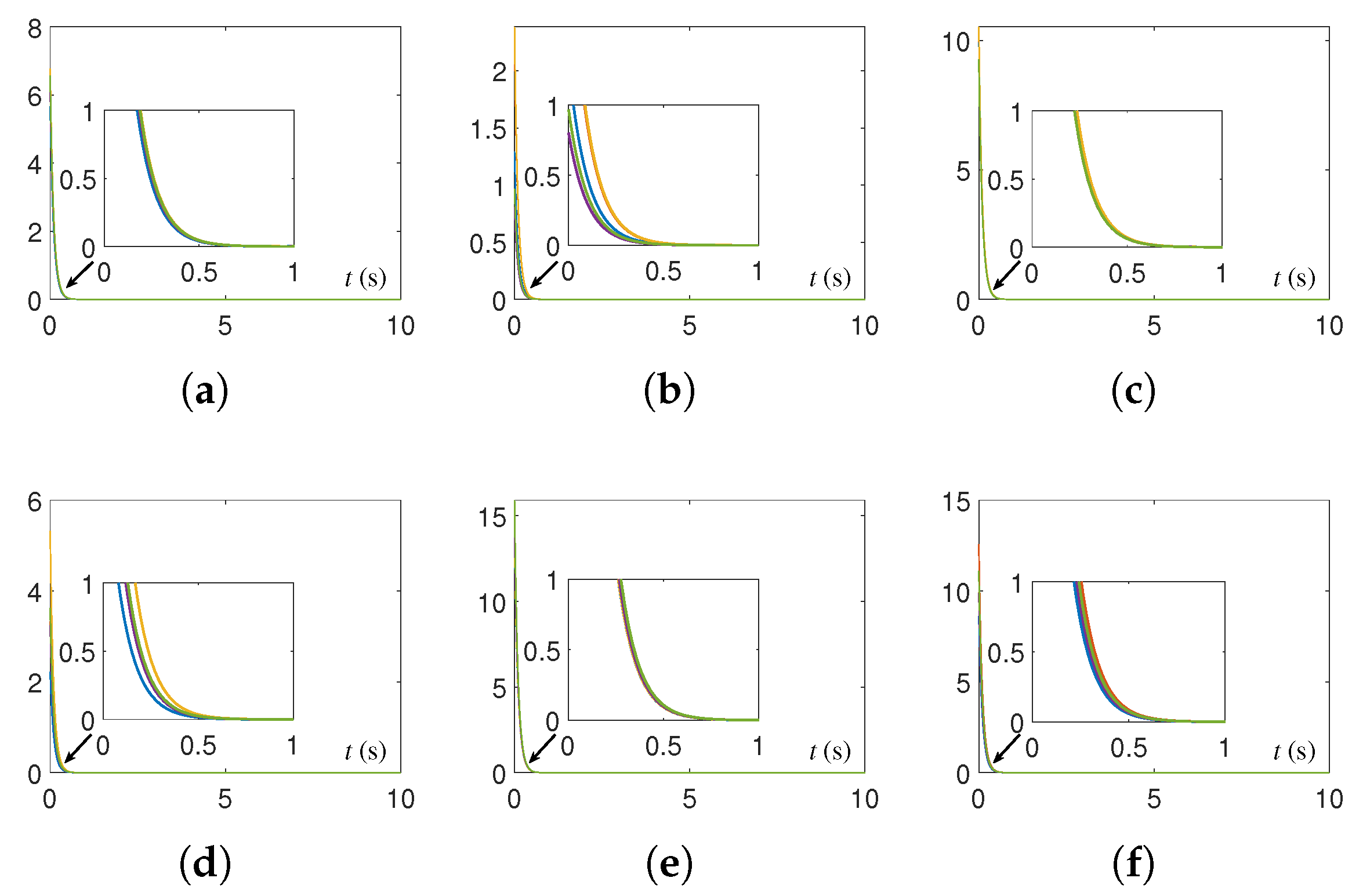
The CTQRD model (5) is implemented by using the ODE (ordinary differential equation) solver [37] in MATLAB routine. Specifically, the ODE function “ode45” is applied in this paper, and the numerical experimental results are shown in Figure 1, Figure 2, Figure 3, Figure 4, Figure 5, Figure 6, Figure 7 and Figure 8. Note that, in Figure 1, Figure 2, Figure 3, Figure 4, Figure 5, Figure 6, Figure 7 and Figure 8, the solution trajectories and residual errors corresponding to different initial values are represented in different colors. From Figure 1, Figure 2, Figure 3 and Figure 4, we can see that the solution trajectories synthesized by CTQRD model (5) with five random initial values and $\varrho =10$ for Example 1 are indeed time-varying. Additionally, the solution trajectories synthesized by (5) for Examples 2 and 3 are omitted because of the space limitation and similarity. As shown in Figure 5, Figure 6 and Figure 7, the residual errors of CTQRD model (5) for Examples 1 through 3 converge to near-zero rapidly, which means Theorem 2 is correct. Meanwhile, the residual error trajectories of the original equivalence problem shown in Figure 8 verify the correctness of this theorem again.

Figure 1. Solution trajectories of $Q_R\left(t\right)$ synthesized by CTQRD model (5) with five random initial values and $\varrho =10$ for Example 1.

Figure 2. Solution trajectories of $Q_I\left(t\right)$ synthesized by CTQRD model (5) with five random initial values and $\varrho =10$ for Example 1.

Figure 3. Solution trajectories of $R_R\left(t\right)$ synthesized by CTQRD model (5) with five random initial values and $\varrho =10$ for Example 1.

Figure 4. Solution trajectories of $R_I\left(t\right)$ synthesized by CTQRD model (5) with five random initial values and $\varrho =10$ for Example 1.

Figure 5. Residual errors of CTQRD model (5) with five random initial values and $\varrho =10$ for Example 1.

Figure 6. Residual errors of CTQRD model (5) with five random initial values and $\varrho =10$ for Example 2.

Figure 7. Residual errors of CTQRD model (5) with five random initial values and $\varrho =10$ for Example 3.

Figure 8. Residual errors of original equivalence problem corresponding to CTQRD model (5) with five random initial values and $\varrho =10$ for Examples 1 through 3. (a) $\left|\right|Q\left(t\right)R\left(t\right)-{C\left(t\right)\left|\right|}_F$ for Example 1. (b) $\left|\right|Q^{*}\left(t\right)Q\left(t\right)-I_m{\left|\right|}_F$ for Example 1. (c) $\left|\right|Q\left(t\right)R\left(t\right)-{C\left(t\right)\left|\right|}_F$ for Example 2. (d) $\left|\right|Q^{*}\left(t\right)Q\left(t\right)-I_m{\left|\right|}_F$ for Example 2. (e) $\left|\right|Q\left(t\right)R\left(t\right)-{C\left(t\right)\left|\right|}_F$ for Example 3. (f) $\left|\right|Q^{*}\left(t\right)Q\left(t\right)-I_m{\left|\right|}_F$ for Example 3.

5.3. DTQRD Models

Note that the DTQRD-1 (11), -2 (12), -3 (13), -4 (14), and -5 (15) models, respectively, require one, three, five, seven, and ten initial values before we can use them. Since the first initial value is randomly generated, the Euler method is adopted to compute these values, except the DTQRD-1 (11) model, which needs one initial value only. Additionally, the solution trajectories synthesized by DTQRD models are not given since the space limitation and similarity.

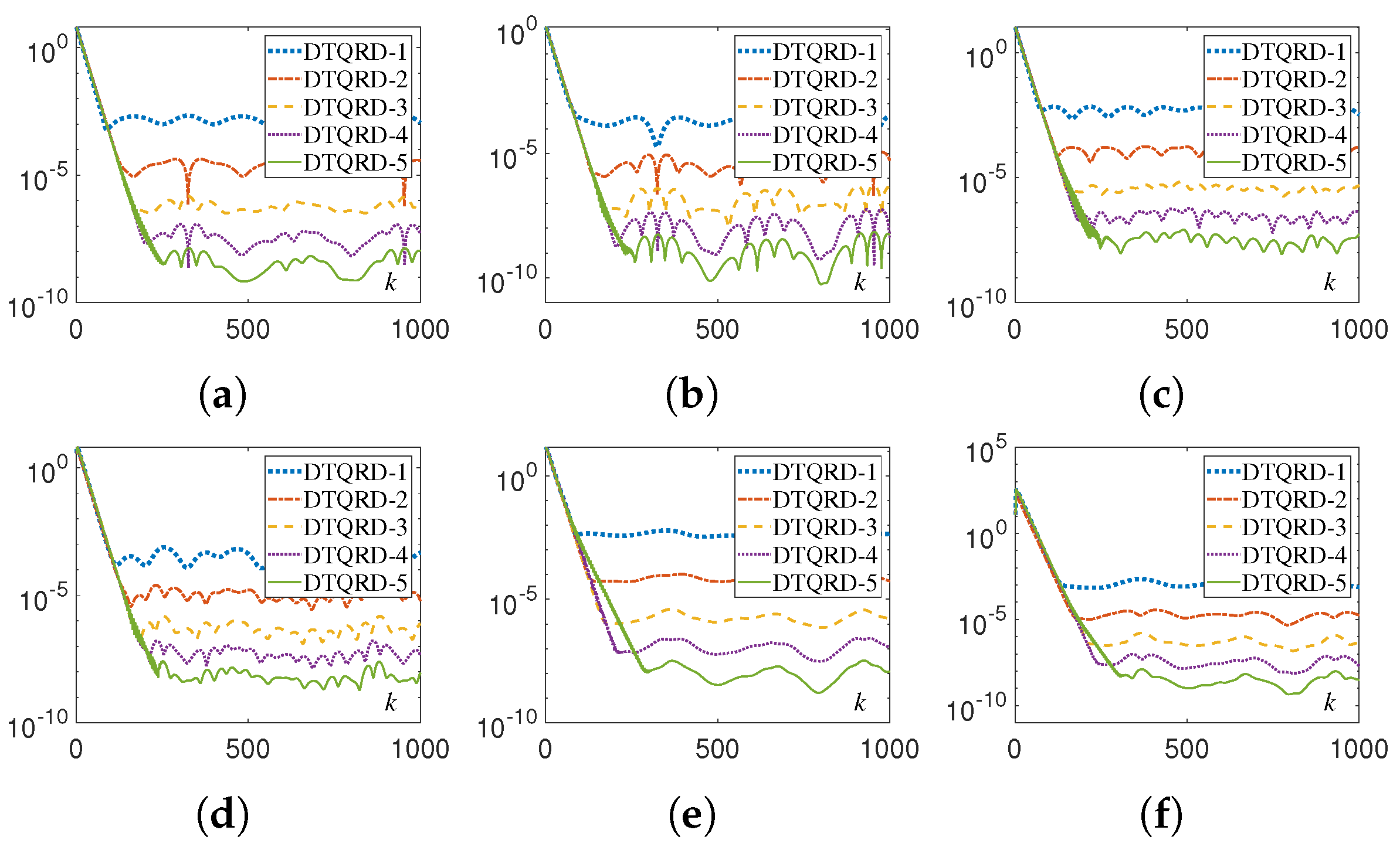
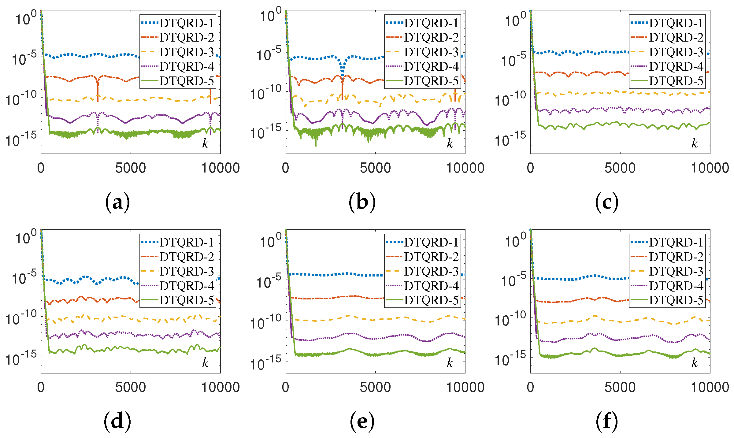
The numerical experimental results for DTQRD models are shown in Figure 9, Figure 10, Figure 11, Figure 12, Figure 13, Figure 14, Figure 15 and Figure 16 and Table 1 and Table 2. Note that, in these tables, we use the MATLAB notation form, i.e., “E” denotes “$\times 10$”. As seen in Figure 9, Figure 10, Figure 11, Figure 12, Figure 13 and Figure 14, the residual error trajectories synthesized by different DTQRD models change regularly, which is consistent with the conclusion of Theorem 4. From the results in Table 1, we know that the residual errors of (11)–(15) are almost proportional to $O\left({\tau }^2\right)$, $O\left({\tau }^3\right)$, $O\left({\tau }^4\right)$, $O\left({\tau }^5\right)$, and $O\left({\tau }^6\right)$, respectively, which also verifies Theorem 4. Moreover, from Figure 15 and Figure 16 as well as Table 2, we can see that the residual errors of the original equivalence problem corresponding to (11)–(15) change in the manner of $O\left({\tau }^2\right)$, $O\left({\tau }^3\right)$, $O\left({\tau }^4\right)$, $O\left({\tau }^5\right)$, and $O\left({\tau }^6\right)$, respectively. Thus, the correctness of Theorem 4 is substantiated.

Figure 9. Residual errors of different DTQRD models with same random initial value, $h=0.1$, and $\tau =0.01s$ for Example 1.

Figure 10. Residual errors of different DTQRD models with same random initial value, $h=0.1$, and $\tau =0.001s$ for Example 1.

Figure 11. Residual errors of different DTQRD models with same random initial value, $h=0.1$, and $\tau =0.01s$ for Example 2.

Figure 12. Residual errors of different DTQRD models with same random initial value, $h=0.1$, and $\tau =0.001s$ for Example 2.

Figure 13. Residual errors of different DTQRD models with same random initial value, $h=0.1$, and $\tau =0.01s$ for Example 3.

Figure 14. Residual errors of different DTQRD models with same random initial value, $h=0.1$, and $\tau =0.001s$ for Example 3.

Figure 15. Residual errors of original equivalence problem corresponding to different DTQRD models with same random initial value, $h=0.1$, and $\tau =0.01s$ for Examples 1 through 3. (a) $\left|\right|Q\left(t_k\right)R\left(t_k\right)-C\left(t_k\right){\left|\right|}_F$ for Example 1. (b) $\left|\right|Q^{*}\left(t_k\right)Q\left(t_k\right)-I_m{\left|\right|}_F$ for Example 1. (c) $\left|\right|Q\left(t_k\right)R\left(t_k\right)-C\left(t_k\right){\left|\right|}_F$ for Example 2. (d) $\left|\right|Q^{*}\left(t_k\right)Q\left(t_k\right)-I_m{\left|\right|}_F$ for Example 2. (e) $\left|\right|Q\left(t_k\right)R\left(t_k\right)-C\left(t_k\right){\left|\right|}_F$ for Example 3. (f) $\left|\right|Q^{*}\left(t_k\right)Q\left(t_k\right)-I_m{\left|\right|}_F$ for Example 3.

Figure 16. Residual errors of original equivalence problem corresponding to different DTQRD models with same random initial value, $h=0.1$, and $\tau =0.001s$ for Examples 1 through 3. (a) $\left|\right|Q\left(t_k\right)R\left(t_k\right)-C\left(t_k\right){\left|\right|}_F$ for Example 1. (b) $\left|\right|Q^{*}\left(t_k\right)Q\left(t_k\right)-I_m{\left|\right|}_F$ for Example 1. (c) $\left|\right|Q\left(t_k\right)R\left(t_k\right)-C\left(t_k\right){\left|\right|}_F$ for Example 2. (d) $\left|\right|Q^{*}\left(t_k\right)Q\left(t_k\right)-I_m{\left|\right|}_F$ for Example 2. (e) $\left|\right|Q\left(t_k\right)R\left(t_k\right)-C\left(t_k\right){\left|\right|}_F$ for Example 3. (f) $\left|\right|Q^{*}\left(t_k\right)Q\left(t_k\right)-I_m{\left|\right|}_F$ for Example 3.

Table 1. Residual errors of different DTQRD models with $h=0.1$.

Model		$\mathit{\tau }\left(\mathit{s}\right)$	Example 1	Example 2	Example 3
DTQRD-1 (11)	$\left|\right|Z_1\left(t_k\right){\left|\right|}_F$	$0.01$	$1.993$E$-03$${}^{\#}$	$4.798$E$-03$	$4.170$E$-03$
		$0.001$	$2.124$E$-05$	$4.621$E$-05$	$4.214$E$-05$
	$\left|\right|Z_2\left(t_k\right){\left|\right|}_F$	$0.01$	$7.199$E$-04$	$4.642$E$-03$	$4.701$E$-03$
		$0.001$	$7.287$E$-06$	$4.851$E$-05$	$4.769$E$-05$
	$\left|\right|Z_3\left(t_k\right){\left|\right|}_F$	$0.01$	$2.845$E$-04$	$6.312$E$-04$	$1.837$E$-03$
		$0.001$	$2.925$E$-06$	$7.525$E$-06$	$1.932$E$-05$
	$\left|\right|Z_4\left(t_k\right){\left|\right|}_F$	$0.01$	$2.626$E$-05$	$1.923$E$-04$	$1.310$E$-03$
		$0.001$	$5.222$E$-07$	$2.957$E$-06$	$1.230$E$-05$
DTQRD-2 (12)	$\left|\right|Z_1\left(t_k\right){\left|\right|}_F$	$0.01$	$4.042$E$-05$	$1.228$E$-04$	$8.062$E$-05$
		$0.001$	$4.371$E$-08$	$1.311$E$-07$	$8.527$E$-08$
	$\left|\right|Z_2\left(t_k\right){\left|\right|}_F$	$0.01$	$1.334$E$-05$	$1.310$E$-04$	$7.616$E$-05$
		$0.001$	$1.445$E$-08$	$1.427$E$-07$	$8.131$E$-08$
	$\left|\right|Z_3\left(t_k\right){\left|\right|}_F$	$0.01$	$8.740$E$-06$	$1.630$E$-05$	$2.772$E$-05$
		$0.001$	$9.919$E$-09$	$2.663$E$-08$	$2.788$E$-08$
	$\left|\right|Z_4\left(t_k\right){\left|\right|}_F$	$0.01$	$1.133$E$-06$	$8.212$E$-06$	$2.242$E$-05$
		$0.001$	$2.395$E$-09$	$1.021$E$-08$	$2.537$E$-08$
DTQRD-3 (13)	$\left|\right|Z_1\left(t_k\right){\left|\right|}_F$	$0.01$	$1.426$E$-06$	$3.500$E$-06$	$2.532$E$-06$
		$0.001$	$1.629$E$-10$	$4.022$E$-10$	$2.732$E$-10$
	$\left|\right|Z_2\left(t_k\right){\left|\right|}_F$	$0.01$	$4.417$E$-07$	$5.896$E$-06$	$3.182$E$-06$
		$0.001$	$4.931$E$-11$	$6.737$E$-10$	$3.463$E$-10$
	$\left|\right|Z_3\left(t_k\right){\left|\right|}_F$	$0.01$	$3.945$E$-07$	$9.573$E$-07$	$1.274$E$-06$
		$0.001$	$4.650$E$-11$	$1.659$E$-10$	$1.385$E$-10$
	$\left|\right|Z_4\left(t_k\right){\left|\right|}_F$	$0.01$	$6.494$E$-08$	$4.612$E$-07$	$1.017$E$-06$
		$0.001$	$1.378$E$-11$	$6.502$E$-11$	$1.077$E$-10$
DTQRD-4 (14)	$\left|\right|Z_1\left(t_k\right){\left|\right|}_F$	$0.01$	$1.129$E$-07$	$3.245$E$-07$	$1.841$E$-07$
		$0.001$	$1.352$E$-12$	$4.127$E$-12$	$2.142$E$-12$
	$\left|\right|Z_2\left(t_k\right){\left|\right|}_F$	$0.01$	$3.671$E$-08$	$5.269$E$-07$	$1.940$E$-07$
		$0.001$	$4.155$E$-13$	$6.199$E$-12$	$2.309$E$-12$
	$\left|\right|Z_3\left(t_k\right){\left|\right|}_F$	$0.01$	$4.153$E$-08$	$1.044$E$-07$	$8.269$E$-08$
		$0.001$	$4.893$E$-13$	$1.873$E$-12$	$8.436$E$-13$
	$\left|\right|Z_4\left(t_k\right){\left|\right|}_F$	$0.01$	$7.821$E$-09$	$4.436$E$-08$	$5.104$E$-08$
		$0.001$	$1.894$E$-13$	$8.657$E$-13$	$6.759$E$-13$
DTQRD-5 (15)	$\left|\right|Z_1\left(t_k\right){\left|\right|}_F$	$0.01$	$1.350$E$-08$	$4.860$E$-08$	$2.005$E$-08$
		$0.001$	$1.954$E$-14$	$6.390$E$-14$	$2.408$E$-14$
	$\left|\right|Z_2\left(t_k\right){\left|\right|}_F$	$0.01$	$3.051$E$-09$	$6.716$E$-08$	$2.649$E$-08$
		$0.001$	$5.037$E$-15$	$8.377$E$-14$	$3.129$E$-14$
	$\left|\right|Z_3\left(t_k\right){\left|\right|}_F$	$0.01$	$5.443$E$-09$	$1.416$E$-08$	$1.107$E$-08$
		$0.001$	$7.664$E$-15$	$3.021$E$-14$	$1.176$E$-14$
	$\left|\right|Z_4\left(t_k\right){\left|\right|}_F$	$0.01$	$1.136$E$-09$	$7.743$E$-09$	$6.601$E$-09$
		$0.001$	$3.317$E$-15$	$9.236$E$-15$	$9.590$E$-15$

#Note: “E” denotes “$\times 10$”, such as “$1.993$E$-03$” denoting “$1.993\times {10}^{-03}$”.

Table 2. Residual errors of original equivalence problem for different DTQRD models with $h=0.1$.

Model		$\mathit{\tau }\left(\mathit{s}\right)$	Example 1	Example 2	Example 3
DTQRD-1 (11)	$\left|\right|Q\left(t_k\right)R\left(t_k\right)-C\left(t_k\right){\left|\right|}_F$	$0.01$	$2.187$E$-03$${}^{\#}$	$6.442$E$-03$	$6.164$E$-03$
		$0.001$	$2.246$E$-05$	$6.672$E$-05$	$6.240$E$-05$
	$\left|\right|Q^{*}\left(t_k\right)Q\left(t_k\right)-I_m{\left|\right|}_F$	$0.01$	$2.878$E$-04$	$6.463$E$-04$	$2.237$E$-03$
		$0.001$	$2.952$E$-06$	$8.061$E$-06$	$2.290$E$-05$
DTQRD-2 (12)	$\left|\right|Q\left(t_k\right)R\left(t_k\right)-C\left(t_k\right){\left|\right|}_F$	$0.01$	$4.341$E$-05$	$1.721$E$-04$	$1.035$E$-04$
		$0.001$	$4.604$E$-08$	$1.871$E$-07$	$1.097$E$-07$
	$\left|\right|Q^{*}\left(t_k\right)Q\left(t_k\right)-I_m{\left|\right|}_F$	$0.01$	$8.981$E$-06$	$1.730$E$-05$	$3.563$E$-05$
		$0.001$	$1.017$E$-08$	$2.858$E$-08$	$3.757$E$-08$
DTQRD-3 (13)	$\left|\right|Q\left(t_k\right)R\left(t_k\right)-C\left(t_k\right){\left|\right|}_F$	$0.01$	$1.493$E$-06$	$6.826$E$-06$	$4.007$E$-06$
		$0.001$	$1.703$E$-10$	$7.772$E$-10$	$4.328$E$-10$
	$\left|\right|Q^{*}\left(t_k\right)Q\left(t_k\right)-I_m{\left|\right|}_F$	$0.01$	$3.984$E$-07$	$9.711$E$-07$	$1.627$E$-06$
		$0.001$	$4.850$E$-11$	$1.824$E$-10$	$1.755$E$-10$
DTQRD-4 (14)	$\left|\right|Q\left(t_k\right)R\left(t_k\right)-C\left(t_k\right){\left|\right|}_F$	$0.01$	$1.195$E$-07$	$6.046$E$-07$	$2.471$E$-07$
		$0.001$	$1.406$E$-12$	$7.448$E$-12$	$2.931$E$-12$
	$\left|\right|Q^{*}\left(t_k\right)Q\left(t_k\right)-I_m{\left|\right|}_F$	$0.01$	$4.306$E$-08$	$1.064$E$-07$	$9.681$E$-08$
		$0.001$	$5.230$E$-13$	$2.062$E$-12$	$1.062$E$-12$
DTQRD-5 (15)	$\left|\right|Q\left(t_k\right)R\left(t_k\right)-C\left(t_k\right){\left|\right|}_F$	$0.01$	$1.389$E$-08$	$8.279$E$-08$	$3.238$E$-08$
		$0.001$	$1.972$E$-14$	$1.041$E$-13$	$3.843$E$-14$
	$\left|\right|Q^{*}\left(t_k\right)Q\left(t_k\right)-I_m{\left|\right|}_F$	$0.01$	$5.559$E$-09$	$1.479$E$-08$	$1.285$E$-08$
		$0.001$	$8.217$E$-15$	$3.414$E$-14$	$1.487$E$-14$

#Note: “E” denotes “$\times 10$”, such as “$2.187$E$-03$” denoting “$2.187\times {10}^{-03}$”.

6. Conclusions

The time-varying QR decomposition in complex domain has been analyzed and investigated in this paper. Firstly, the new CTQRD model has been derived and proposed by adopting the ZND method as well as the dimensional reduction method, equivalent transformations, Kronecker product, and vectorization techniques. In addition, the novel eleven-instant ZeaD formula, with $O\left({\tau }^5\right)$ precision, has been proposed. Then, by using the eleven-instant and other ZeaD formulas, five DTQRD models have been further proposed and studied. The theoretical analysis has indicated the correctness of the CTQRD and DTQRD models. Finally, the numerical experimental results have substantiated the effectiveness and precision of the proposed continuous and discrete models. Our future research will focus on building a unified/hybrid model or platform that can solve the time-varying QR decomposition with both continuous and discrete time conditions. In addition, other types of time-varying matrix decomposition problems are also one of our future research directions.

References

1. Jadhav, S.; Zhao, J.; Fan, Y.; Li, J.; Lin, H.; Yan, C.; Chen, M. Time-varying sequence model. Mathematics 2023, 11, 336. [Google Scholar] [CrossRef]
2. Masubuchi, I.; Kikuchi, T. Lyapunov density criteria for time-varying and periodically time-varying nonlinear systems with converse results. SIAM J. Control Optim. 2021, 59, 223–241. [Google Scholar] [CrossRef]
3. Li, X.; Cao, J. An inpulsive delay inequality involving unbounded time-varying delay and applicaitons. IEEE Trans. Autom. Control 2017, 62, 3618–3625. [Google Scholar] [CrossRef]
4. Rios-Rivera, D.; Rios, J.; Sanchez, O.; Alanis, A. Impulsive pinning control of discrete-time complex network with time-varying connections. Mathematics 2022, 10, 4051. [Google Scholar] [CrossRef]
5. Liu, X.; Li, W.; Yao, C.; Li, Y. Finite-time guaranteed cost control for markovian jump systems with time-varying delays. Mathematics 2022, 10, 2028. [Google Scholar] [CrossRef]
6. Guo, D.; Lin, X. Li-function activated Zhang neural network for online solution of time-varying linear matrix inequality. Neural Process Lett. 2020, 52, 713–726. [Google Scholar] [CrossRef]
7. Jerbi, H.; Alharbi, H.; Omri, M.; Ladhar, L.; Simos, T.E.; Mourtas, S.D.; Katsikis, V.N. Towards higher-order zeroing neural network dynamics for solving time-varying algebraic Riccati equations. Mathematics 2022, 10, 4490. [Google Scholar] [CrossRef]
8. Liao, B.; Hua, C.; Cao, X.; Katsikis, V.N.; Li, S. Complex noise-resistant zeroing neural network for computing complex time-dependent Lyapunov equation. Mathematics 2022, 10, 2817. [Google Scholar] [CrossRef]
9. Jin, L.; Li, S.; Xiao, L.; Lu, R.; Liao, B. Cooperative motion generation in a distributed network of redundant robot manipulators with noises. IEEE Trans. Syst. Man Cybern. 2018, 48, 1715–1724. [Google Scholar] [CrossRef]
10. Zhang, Z.; Chen, B.; Luo, Y. A deep ensemble dynamic learning network for corona virus disease 2019 diagnosis. IEEE Trans. Neural Netw. Learn. Syst. 2023, in press. [Google Scholar] [CrossRef]
11. Uhlig, F. Zhang neural network for fast and accurate computations of the field of values. Linear Multilinear A. 2019, 68, 1894–1910. [Google Scholar] [CrossRef] [Green Version]
12. Li, J.; Shi, Y.; Xuan, H. Unified model solving nine types of time-varying problems in the frame of zeroing neural network. IEEE Trans. Neural Netw. Learn. Syst. 2021, 32, 1896–1905. [Google Scholar] [CrossRef] [PubMed]
13. Xiao, L.; He, Y.; Dai, J.; Liu, X.; Liao, B.; Tan, H. A variable-parameter noise-tolerant zeroing neural network for time-variant matrix inversion with guaranteed robustness. IEEE Trans. Neural Netw. Learn. Syst. 2022, 33, 1535–1545. [Google Scholar] [CrossRef]
14. Liao, B.; Han, L.; He, Y.; Cao, X.; Li, J. Prescribed-time convergent adaptive ZNN for time-varying matrix inversion under harmonic noise. Electronics 2022, 11, 1636. [Google Scholar] [CrossRef]
15. Zheng, L.; Zhang, Z. Time-varying quadratic-programming-based error redefinition neural network control and its application to mobile redundant manipulators. IEEE Trans. Autom. Control 2022, 67, 6151–6158. [Google Scholar] [CrossRef]
16. Jin, L.; Zhang, Y. Continuous and discrete Zhang dynamics for real-time varying nonlinear optimizaiton. Numer. Algor. 2016, 73, 115–140. [Google Scholar] [CrossRef]
17. Uhlig, F. Time-varying matrix eigenanalyses via Zhang neural networks and look-ahead finite difference equations. Linear Algebr. Appl. 2019, 580, 417–435. [Google Scholar] [CrossRef] [Green Version]
18. Uhlig, F. The construction of high order convergent look-ahead finite difference formulas for Zhang neural networks. J. Differ. Equ. Appl. 2019, 25, 931–941. [Google Scholar] [CrossRef] [Green Version]
19. Xuan, H.; Zhu, X.; Li, J.; Guo, H.; Li, Y. General third-order-accuracy formulas for time discretization applied to time-varying optimization. IEEE Access 2020, 8, 224235–224245. [Google Scholar] [CrossRef]
20. Sun, M.; Wang, Y. General five-step discrete-time Zhang neural network for time-varying nonlinear optimization. Bull. Malays. Math. Sci. Soc. 2020, 43, 1741–1760. [Google Scholar] [CrossRef]
21. Sun, M.; Liu, J. General six-step discrete-time Zhang neural network for time-varying tensor absolute value equations. Discrete Dyn. Nat. Soc. 2019, 2019, 1–12. [Google Scholar] [CrossRef] [Green Version]
22. Hu, C.; Kang, X.; Zhang, Y. Three-step general discrete-time Zhang neural network design and application to time-variant matrix inversion. Neurocomputing 2018, 306, 108–118. [Google Scholar] [CrossRef]
23. Guo, D.; Nie, Z.; Yan, L. Novel discrete-time Zhang neural network for time-varying matrix inversion. IEEE Trans. Syst. Man Cybern. 2017, 47, 2301–2310. [Google Scholar] [CrossRef]
24. Chen, J.; Zhang, Y. Discrete-time ZND models solving ALRMPC via eight-instant general and other formulas of ZeaD. IEEE Access 2019, 7, 125909–125918. [Google Scholar] [CrossRef]
25. Liu, Y.; Tian, Y. A simultaneous decomposition of a matrix triplet with applications. Numer. Linear Algebr. 2011, 18, 69–85. [Google Scholar] [CrossRef]
26. Foster, J.; McWhirter, J.; Davies, M.; Chambers, J. An algorithm for calculating the QR and singular value decompositions of polynomial matrices. IEEE Trans. Signal Process. 2010, 58, 1263–1274. [Google Scholar] [CrossRef] [Green Version]
27. Merino, D.; Paras, A.; Pelejo, D. On the phi(J) polar decomposition of matrices. Linear Algebr. Appl. 2010, 432, 1165–1175. [Google Scholar] [CrossRef] [Green Version]
28. Li, F. On the Jacobians of singular matrix decomposition and its application. Linear Multilinear A 2021, 69, 1521–1533. [Google Scholar] [CrossRef]
29. Baumann, M.; Helmke, U. Singular value decomposition of time-varying matrices. Future Gen. Comput. Syst. 2003, 19, 353–361. [Google Scholar] [CrossRef]
30. Tănăsescu, A.; Carabaş, M.; Pop, F.; Popescu, P.G. Scalability of K-tridiagonal matrix singular value decomposition. Mathematics 2021, 9, 3123. [Google Scholar] [CrossRef]
31. Alharbi, H.; Jerbi, H.; Kchaou, M.; Abbassi, R.; Simos, T.E.; Mourtas, S.D.; Katsikis, V.N. Time-varying pseudoinversion based on full-rank decomposition and zeroing neural networks. Mathematics 2023, 11, 600. [Google Scholar] [CrossRef]
32. Chen, J.; Zhang, Y. Online singular value decomposition of time-varying matrix via zeroing neural dynamics. Neurocomputing 2020, 383, 314–323. [Google Scholar] [CrossRef]
33. Katsikis, V.N.; Mourtas, S.D.; Stanimirovic, P.S.; Zhang, Y. Continuous-time varying complex QR decomposition via zeroing neural dynamics. Neural Process. Lett. 2021, 53, 3573–3590. [Google Scholar] [CrossRef]
34. Li, Z.; Zhang, Y.; Ming, L.; Guo, J.; Katsikis, V.N. Real-domain QR decomposition models employing zeroing neural network and time-discretization formulas for time-varying matrices. Neurocomputing 2021, 448, 217–227. [Google Scholar] [CrossRef]
35. Katsikis, V.N.; Mourtas, S.D.; Stanimirovic, P.S.; Zhang, Y. Solving complex-valued time-varying linear matrix equations via QR decomposition with applications to robotic motion tracking and on angle-of-arrival localization. IEEE Trans. Neural Netw. Learn. Syst. 2022, 33, 3415–3424. [Google Scholar] [CrossRef]
36. Horn, R.A.; Johnson, C.R. Topics in Matrix Analysis; Cambridge University Press: New York, NY, USA, 1991. [Google Scholar]
37. Mathews, J.H.; Fink, K.D. Numerical Methods Using MATLAB; Prentice-Hall: Englewood Cliffs, NJ, USA, 2004. [Google Scholar]
38. Griffiths, D.F.; Higham, D.J. Numerical Methods for Ordinary Differential Equations: Initial Value Problems; Springer: London, UK, 2010. [Google Scholar]
39. Suli, E.; Mayers, D.F. An Introduction to Numerical Analysis; Cambridge University Press: Oxford, UK, 2003. [Google Scholar]
Figure 1. Solution trajectories of Q R ( t ) synthesized by CTQRD model (5) with five random initial values and ϱ = 10 for Example 1.
Mathematics 11 03354 g001
Figure 2. Solution trajectories of Q I ( t ) synthesized by CTQRD model (5) with five random initial values and ϱ = 10 for Example 1.
Mathematics 11 03354 g002
Figure 3. Solution trajectories of R R ( t ) synthesized by CTQRD model (5) with five random initial values and ϱ = 10 for Example 1.
Mathematics 11 03354 g003
Figure 4. Solution trajectories of R I ( t ) synthesized by CTQRD model (5) with five random initial values and ϱ = 10 for Example 1.
Mathematics 11 03354 g004