Article

An Alternate GPU-Accelerated Algorithm for Very Large Sparse LU Factorization

School of Geophysics and Geomatics, China University of Geosciences, Wuhan 430074, China
*
Author to whom correspondence should be addressed.
Mathematics 2023, 11(14), 3149; https://doi.org/10.3390/math11143149
Submission received: 7 June 2023 / Revised: 10 July 2023 / Accepted: 13 July 2023 / Published: 17 July 2023
(This article belongs to the Section E: Applied Mathematics)

Abstract

:
The LU factorization of very large sparse matrices requires a significant amount of computing resources, including memory and broadband communication. A hybrid MPI + OpenMP + CUDA algorithm named SuperLU3D can efficiently compute the LU factorization with GPU acceleration. However, this algorithm faces difficulties when dealing with very large sparse matrices with limited GPU resources. Factorizing very large matrices involves a vast amount of nonblocking communication between processes, often leading to a break in SuperLU3D calculation due to the overflow of cluster communication buffers. In this paper, we present an improved GPU-accelerated algorithm named SuperLU3D_Alternate for the LU factorization of very large sparse matrices with fewer GPU resources. The basic idea is “divide and conquer”, which means dividing a very large matrix into multiple submatrices, performing LU factorization on each submatrix, and then assembling the factorized results of all submatrices into two complete matrices L and U. In detail, according to the number of available GPUs, a very large matrix is first divided into multiple submatrices using the elimination tree. Then, the LU factorization of each submatrix is alternately computed with limited GPU resources, and its intermediate LU factors from GPUs are saved to the host memory or hard disk. Finally, after finishing the LU factorization of all submatrices, these factorized submatrices are assembled into a complete lower triangular matrix L and a complete upper triangular matrix U, respectively. The SuperLU3D_Alternate algorithm is suitable for hybrid CPU/GPU cluster systems, especially for a subset of nodes without GPUs. To accommodate different hardware resources in various clusters, we designed the algorithm to run in the following three cases: sufficient memory for GPU nodes, insufficient memory for GPU nodes, and insufficient memory for the entire cluster. The results from LU factorization test on different matrices in various cases show that the larger the matrix is, the more efficient this algorithm is under the same GPU memory consumption. In our numerical experiments, SuperLU3D_Alternate achieves speeds of up to 8× that of SuperLU3D (CPU only) and 2.5× that of SuperLU3D (CPU + GPU) on the hybrid cluster with six Tesla V100S GPUs. Furthermore, when the matrix is too big to be handled by SuperLU3D, SuperLU3D_Alternate can still utilize the cluster’s host memory or hard disk to solve it. By reducing the amount of data exchange to prevent exceeding the buffer’s limit of the cluster MPI nonblocking communication, our algorithm enhances the stability of the program.

1. Introduction

Numerical problems often require the solution of large sparse systems of linear equations, such as those found in finite difference approximations of three-dimensional partial differential equations [1]. These computations can be time-consuming, and the most important part of the process is solving these large systems of equations. There are two main categories of methods for solving such systems: direct and iterative. Direct solvers include MUMPS (Multifrontal Massively Parallel Sparse Direct Solver) [1,2], PARDISO [3], and SuperLU (Supernodal Lower-Upper Factorization) [4,5,6,7]. The common iterative solvers are PETSc (Portable, Extensible Toolkit for Scientific Computation) [8], Trilinos [9], and HYPRE (High-Performance Preconditioners) [10]. However, iterative methods may suffer from slow convergence or divergence issues when dealing with complex matrices, whereas direct methods require high computing resources. In certain simulations, such as three-dimensional geodynamical simulations [11,12,13,14], solving a system of linear partial differential equations comprising the Stokes equations and mass continuity equations can result in matrices with hundreds of millions of dimensions. If the number of model grids is 500 × 500 × 100, it will require over 1 TB of host memory and 1 TB of GPU memory for traditional direct solvers with GPU acceleration. As the number of grids and computing accuracy increases, so does the demand for computing resources, making it difficult for small- and medium-sized clusters to solve such problems.
The solution of Ax = b using the LU factorization method is divided into two logical steps. The first step is to factorize matrix A into the product of a lower triangular matrix L and an upper triangular matrix U. The second step is to obtain the solution x of the system of equations by solving L y = b and then solving Ux = y . Since a large number of matrix operations are needed in LU factorization, GPU acceleration is a great way to significantly improve the computational efficiency.
In solving a very large system of linear equations with GPU acceleration, the first step takes much more time than the second step. Calculating matrices L and U requires a large amount of memory and communication among GPUs. It is challenging to factorize very large sparse matrices efficiently when the computing resources, such as the GPU memory and MPI communication buffer, cannot meet the requirements.
Among LU factorization solvers, the SuperLU solver is a supernode factorization method using a hybrid MPI + OpenMP programming model. The three libraries within SuperLU are Sequential SuperLU, Multithreaded SuperLU (SuperLU_MT), and Distributed SuperLU (SuperLU_DIST). The SuperLU_DIST library contains a 2D and 3D SuperLU_DIST algorithm. The 3D SuperLU_DIST (SuperLU3D) algorithm with GPU acceleration achieves an increased speed of 10~54× and 4.2~6.6× for solving 2D and 3D PDE problems, respectively, compared with the PARDISO parallel algorithm based on MKL (Math Kernel Library) [4,5]. Therefore, making full use of GPU acceleration can greatly improve computational efficiency. Based on SuperLU_DIST, Gaihre introduced the GSOFA algorithm to enable fine-grained symbolic factorization. This algorithm redesigned a supernode detection to expose massive parallelism, balanced workload and minimal inter-node communication, as well as introduced a three-pronged space optimization to handle large sparse matrices [15]. All the SuperLU algorithms are implemented with parallel extensions using OpenMP for shared-memory programming, or MPI + CUDA for distributed-memory programming. The 3D SuperLU_DIST (SuperLU3D) algorithm with GPU acceleration is the most efficient one among these algorithms but faces the difficulty of not being able to solve very large sparse matrices with limited GPU resources, and factorizing very large matrices makes a vast amount of nonblocking communication between processes that can cause a break in the SuperLU3D calculation due to cluster communication buffer overflow.
To address the issues above, we developed a new algorithm called SuperLU3D_Alternate. It uses an approach similar to a time-sharing operating system, where the matrix is divided into submatrices and LU factorization is performed on each submatrix alternately using limited GPU resources. Intermediate LU factors are saved to the host memory or hard disk, and the factorized submatrices are then assembled to form two triangle matrices L and U. In our numerical experiments, SuperLU3D_Alternate achieves speeds of up to 8× that of SuperLU3D (CPU only) and 2.5× that of SuperLU3D (CPU + GPU) on a hybrid cluster with six Tesla V100S GPUs. The new algorithm reduces the amount of data exchange to prevent the cluster’s MPI nonblocking communication buffer from being overloaded, thereby improving the stability of the algorithm. Additionally, if the GPU memory is insufficient for the LU factorization of the entire matrix, SuperLU3D_Alternate can still utilize the cluster’s host memory or hard disk to save the intermediate LU factors of submatrices.

2. SuperLU3D_Alternate Algorithm

2.1. Background

A communication-avoiding 3D algorithm for sparse LU factorization named SuperLU3D in this paper is based on the 2D SuperLU_DIST algorithm. The 2D SuperLU_DIST algorithm is a supernodal factorization parallel algorithm using a hybrid MPI + OpenMP programming model. A supernode is a set of consecutive columns of matrix L with a dense triangular block below the diagonal and with the same nonzero structure below the triangular block (Figure 1) [5,7,15]. Despite its efficiency, 2D SuperLU_DIST has two major limitations that impact its parallel efficiency: the sequential Schur-complement update and fixed latency cost [4]. To address these limitations, the SuperLU3D algorithm uses a 3D logical process grid, which greatly improves its computational efficiency, achieving ~27 times higher efficiency than 2D SuperLU_DIST. SuperLU3D also supports a hybrid architecture with both a multicore CPU and coprocessors such as GPU or Xeon-Phi, with GPU acceleration providing 1.4–3.5 times faster performance on smaller 2D process grids [4]. Furthermore, this algorithm is also applicable to unsymmetrical matrices [6,7]. Table 1 summarizes the symbols used in the subsequent sections.

2.1.1. Elimination Trees

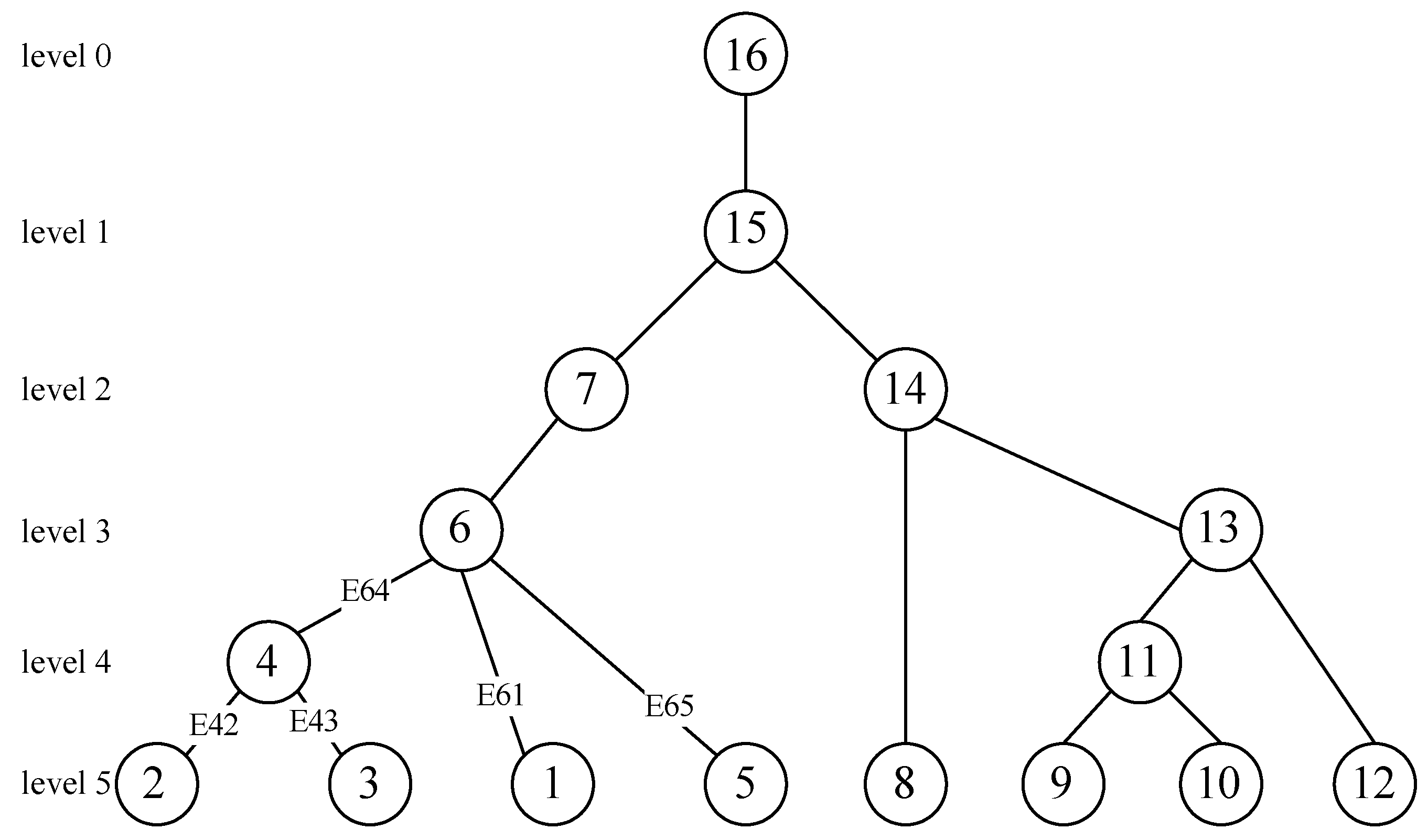
A fundamental concept in sparse matrix factorization is an elimination tree [16]. An n × n symmetric matrix has an n-node elimination tree. The relative position of the matrix elements determines the parent–child relationship among the tree nodes. If the first nonzero element in the j-th column is in the i-th row and i > j, node-i in the tree will be the parent node of node-j. We define this parent–child relationship by connecting node-i and node-j with a line (Figure 2). We express this relationship by
i = p a r e n t j = min { k r o w i n d e x j } , r o w i n d e x j N U L L                               j                                     , r o w i n d e x j = N U L L
where r o w _ i n d e x ( j ) is the number set of rows where nonzero elements in the j-th column are located. We define a 16 × 16 sparse matrix A to illustrate the establishment process of the elimination tree (Figure 2). The blank position of matrix A is zero, and a i j is a nonzero element at the i-th row and j-th column. Sparse LU factorization by columns can be represented by an elimination tree. The dependency of column update is determined by the elimination tree. Therefore, we can utilize elimination trees to compute different subtrees with same parent node concurrently.
A = 1 × × × × 2 × × × × 3 × × × × × × 4 × × × × 5 × × × × × × × 6 × × × × × × × × × 7 × × 8 × × × 9 × × × × 10 × × × × × × 11 × × × × 12 × × × × × × 13 × × × × × × × × × 14 × × × × × × × × × × × × × × × × 15 × × × × × × × × × × × × × × × × 16

2.1.2. Block Algorithm for LU Factorization

We describe the block algorithm for LU factorization in a simplest case. Suppose matrix A is decomposed into 2 × 2 blocks and the equation A = LU can be written as
A 11 A 12 A 21 A 22 = L 11 L 21 L 22 U 11 U 12 U 22 ,
where A is a n × n sparse matrix and A 11 is a d × d sparse matrix (d < n, mod(n, d) = 0).
Based on matrix multiplication, A 11 , A 12 , A 12 , and A 22 can be formulated as
A 11 = L 11 U 11 ,
A 12 = L 11 U 12 ,
A 21 = L 21 U 11 ,
A 22 = L 21 U 12 + L 22 U 22 ,
The steps of the block algorithm for LU factorization are as follows:
(1)
Diagonal factorization: L 11 and U 11 are obtained from LU factorization of block matrix A 11 in Equation (2);
(2)
Panel updates: U 12 = L 11 1 A 12 and L 21 = A 21 U 11 1 ;
(3)
Schur-complement update: L 22 U 22 = A 22 L 21 U 12 , and update A 22 = L 22 U 22 ;
Then, we continue the LU partition factorization of A 22 until the dimension of A 22 is equal to d.

2.1.3. The 2D SuperLU_DIST Algorithm

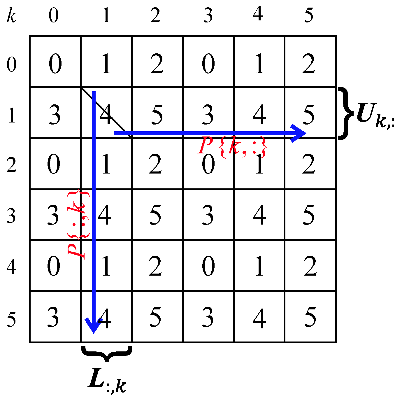
The 2D SuperLU_DIST algorithm was designed for distributed memory parallel processors, using MPI for interprocess communication. It is able to utilize hundreds of parallel processors effectively on sufficiently large matrices [6,17]. It makes one-dimensional MPI processes into a new two-dimensional communicator. The algorithm distributes the supernodal blocks in a two-dimensional P x × P y block-cyclic fashion. This means that block ( I , J ) ( 0 I , J N 1 , N is the number of supernodal blocks) is mapped into the process at coordinate m o d I , P x , m o d j , P y of the 2D P x × P y process grid. The size of each supernodal block can be determined from the dimension of the diagonal matrix in the supernodes. The matrix in Figure 3 illustrates such a partition [18]. More specifically, the algorithm for the k-th supernode involves the following steps [4]:
(1)
Diagonal factorization: The process P k , k factorizes A k k into L k k U k k . The matrix block A k k belongs to P k , k ;
(2)
Diagonal broadcast (blue arrows in Figure 3): the process P k , k broadcasts L k k along its process row P { k , : } to block A k , : , and broadcasts U k k along its process column P { : , k } to block A : , k ;
(3)
Panel solve: Each process in the P { k , : } calculates U k , : = L k k 1 A k , : , and converts the U k , : , which is stored in a sparse format, into a dense format, U ~ k , : (because matrix L : , k is a dense supernode mentioned in Section 2.1). Each process in the P { : , k } calculates L : , k = A : , k U k k 1 ;
(4)
Panel broadcast: each process in P { k , : } or P { : , k } broadcasts blocks of U ~ k , : or L : , k to its process column or row, respectively;
(5)
Schur-complement update: the process P i , j updates A i j by A i j = A i j L i k U ~ k j , where the process P i , j is No. m o d i , P x × P y + m o d j , P y of process.

2.1.4. The SuperLU3D Algorithm

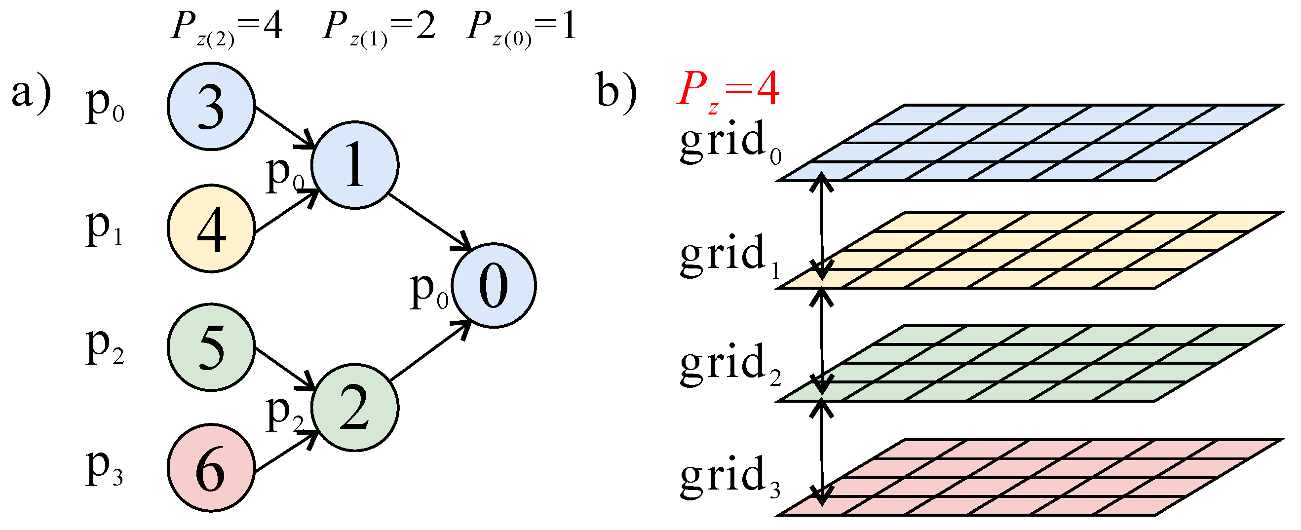
The SuperLU3D algorithm, developed from the 2D SuperLU_DIST algorithm, assigns multiple leaf nodes of an elimination tree to different processes to make smaller independent submatrices, which can reduce the communication cost during the factorization of each submatrix [4]. This is achieved by dividing the elimination tree into independent subtrees and a common ancestor tree of all the subtrees. Each subtree is assigned to a different 2D process grid, while the common ancestor tree is replicated across all process grids to obtain global matrices L and U [4]. As an example, the matrix A in Section 2.1.1 can be divided into two subtrees and a common ancestor tree involving node-16 and node-15.
According to the SuperLU3D algorithm, the matrix A in Section 2.1.1 can be written as
A = A 11 A 13 A 22 A 23 A 31 A 32 A 33 .
Using the elimination tree (Figure 2), we divide the matrix A into two independent submatrices A 0 = A 11 A 13 A 31 A 33 0 and A 1 = A 22 A 23 A 32 A 33 1 . A 11 and A 22 are 7 × 7 matrices, and A 33 0 = A 33 , A 33 1 = 0 . A 0 and A 1 are factorized on 2D process grid-0 and grid-1, respectively, which has the same number of processes (Figure 3). This algorithm considers a collection of 2D grids as a 3D process grid. We refer to the z-dimension of the 3D process grid as P z , which is also equal to the number of submatrices. Based on a block algorithm for LU factorization (Section 2.1.2), after the Schur-complement update in parallel, A 33 0 = A 33 0 L 31 U 13 and A 33 1 = L 32 U 23 . Then, we reduce A 33 1 from grid-1 to grid-0 and update A 33 = A 33 0 + A 33 1 = A 33 0 L 31 U 13 L 32 U 23 . Finally, we factorize A 33 to L 33 and U 33 . Eventually, the L and U of A are distributed among the two process grids. Using the 3D process grid, the SuperLU3D algorithm performs the Schur-complement update of different subtrees or submatrices in parallel [4].

2.2. The SuperLU3D_Alternate Algorithm

In the context of very large matrices, the SuperLU3D algorithm with GPU acceleration faces two major computing problems. Firstly, if there is insufficient GPU memory, all submatrices cannot be decomposed simultaneously. Secondly, the simultaneous decomposition of each submatrix results in extensive nonblocking communication between processes, which may overload the cluster communication buffer and cause program failure. To address these issues, we propose a new algorithm called SuperLU3D_Alternate. The algorithm performs the LU factorization of each submatrix using GPU acceleration alternately, similar to the time-sharing operating system. Another algorithm, GSOFA, also tackles this problem by dividing the submatrix and temporarily buffering some data into the host memory. But all submatrices are still executed in parallel [15].
The SuperLU3D_Alternate algorithm is designed to address the challenges of LU factorization for very large sparse matrices. The algorithm divides the matrix into multiple submatrices using the elimination tree and processes the LU factorization of each submatrix on the same GPUs alternately. During the intermediate process, we synchronize the intermediate L and U of each submatrix in the GPU memory to the host memory or hard disk, and free GPU memory. Once the LU factorization of each submatrix is completed in turn, the submatrices are assembled to form a complete matrix L and a complete matrix U. By decomposing independent submatrices with GPU acceleration, the SuperLU3D_Alternate algorithm provides an efficient and scalable approach to solving very large systems of linear equations.
The implementation details of the SuperLU3D_Alternate algorithm are slightly different in various types of computing environments. To better describe the algorithm, we have the following settings:
(1)
Cluster computing resources: We assume that the hybrid CPU/GPU cluster is composed of m compute nodes. The i-th node has memory M n o d e i and k i k i 0 GPUs with the same video memory size ( M g p u ), where 1 i m . The number of compute nodes of k i > 0 is defined as G P U n o d e n u m , and the nodes are sorted from the largest of k i to the smallest;
(2)
Matrix blocking, process binding, and data structures: For simplicity, it is assumed that the leaf nodes of the elimination tree E are load-balanced on each level, in other words, the amount of computation and storage on each leaf node is almost the same. Moreover, we assume that the levels in E are indexed in the top-down order. Therefore, the parent node index of the tree is zero, while the leaf node index is from 1 to l. At each level, we define E f [ l v l , i ] as the activation state of subtree-i. If the leaf subtrees have been merged to form the parent trees, we will make E f l v l , i = N U L L . We define P = P x y × P z , and P z is the number of 2D process grids, where P z = 2 l . We map each submatrix p i to a 2D process grid ( g r i d i ), so it is equivalent to dividing the total matrix into P z submatrices. Therefore, we consider that the processes are organized in a three-dimensional virtual processor grid with P x rows, P y columns, and P z depths using the MPI Cartesian grid topology construct. Each process has a 3D process coordinate p i d x , p i d y , p i d z . A 2D process grid contains those processes with the same p i d z . It is convenient for processes with the same coordinates p i d x , p i d y to communicate between different 2D process grids. Each process invokes a piece of GPU memory, which is less than M g p u . We bind processes with the same m o d p i d , P x y to the same GPU, where p i d is the MPI rank of process. We use a data structure that consists of sparse matrices and elimination trees, which is the same as the data structure in the SuperLU3D algorithm. The SuperLU3D algorithm uses a principal data structure SuperMatrix to represent a general matrix, sparse or dense. The SuperMatrix structure contains two levels of fields. The first level defines all the properties of a matrix that are independent of how it is stored in memory. The properties contain the storage type, the data type, the number of rows, the number of columns, and a pointer to the actual storage of the matrix (*Store). The second level (*Store) points to the actual storage of the matrix. The *Store points to a structure of four elements that consists of the number of nonzero elements in the matrix, a pointer to an array of nonzero values (*nzval), a pointer to an array of row indices of the nonzeros elements, and a pointer to the array of beginning of columns in nzval[]. The elimination tree is a vector of parent pointers for a forest;
(3)
The per-process host memory and GPU memory, M i h o s t and M i g p u , required to store all the LU factors: For LU factorization of the matrices arising from 2D PDEs, M i h o s t M i g p u 1 P i = 0 l n i 2 2 l + i = l + 1 log n n i 2 2 i ; for LU factorization of those arising from 3D PDEs, M i h o s t M i g p u = i = 0 l 1 n i 2 P x y + i = l log n 2 i n i 2 P [4], where n i is the dimension of the supernodes in the level-i. However, these two equations are not suitable for the matrix with a more complex structure. We can obtain these two memories using the SuperLU3D_Alternate program output instead.
In the case of limited cluster host memory and GPU memory, we must first select the appropriate P x , P y , P z , and n i to guarantee M i g p u M g p u . In addition, the GPU memory size of one submatrix needs to be less than the cluster’s GPU memory size, i.e., P x y M i g p u i = 1 m k i M g p u . Moreover, our algorithm will store the LU factors from GPU device memory in the host memory or hard disk in the intermediate computational steps. Therefore, according to different types of the hybrid CPU/GPU cluster, the algorithm has to face three cases: sufficient memory for GPU nodes ( P M i h o s t + M i g p u < i = 1 n M n o d e i ), insufficient memory for GPU nodes ( i = 1 n M n o d e i < P M i h o s t + M i g p u i = 1 m M n o d e i ), and insufficient memory for the entire cluster ( P M i h o s t + M i g p u > i = 1 m M n o d e i ), where P M i h o s t + M i g p u is the memory required by LU factorization, i = 1 n M n o d e i is the memory of the compute nodes with GPUs, and i = 1 m M n o d e i is the memory of the cluster. We define these three cases as Case A, Case B, and Case C.

2.2.1. Case A: Sufficient Memory for GPU Nodes

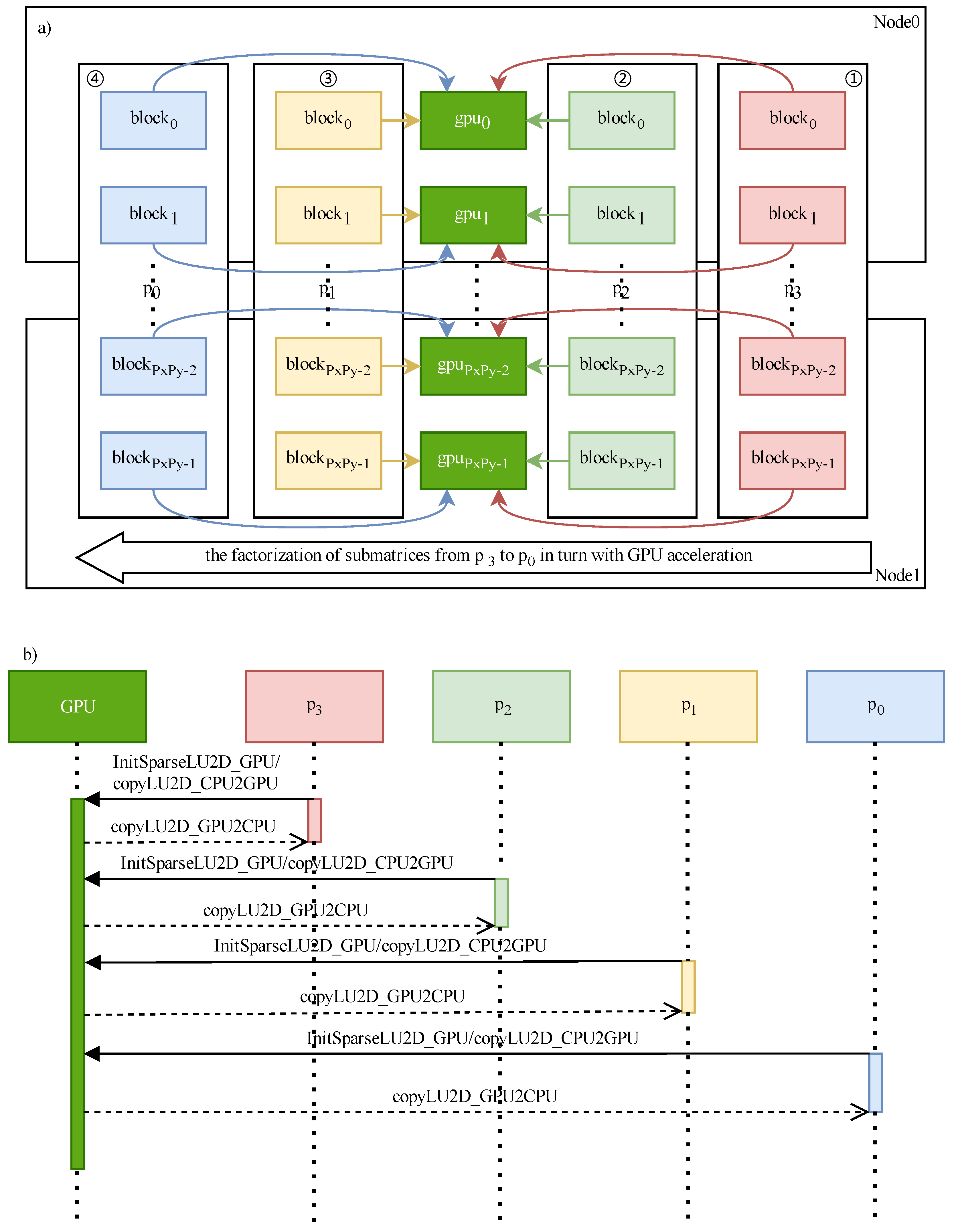
We first consider the simplest case: when all the memory of the nodes with GPUs, which include the host memory and GPU device memory, satisfies the requirement of LU factorization, for which the SuperLU3D_Alternate algorithm needs to save the LU factors from the GPU device memory to the host memory in the intermediate computational steps. Here, we give a simple example to illustrate this case. According to the SuperLU3D algorithm, for example, if the elimination tree only has l = 2 levels, i.e., P z ( l ) = 2 l = 4 , the matrix will be divided Into four submatrices, denoted as p 0 , p 1 , p 2 , and p 3 (Figure 4a). The i-th submatrix is factorized in g r i d i with P x × P y processes (Figure 4b) in compute Node 0 and Node 1 (Figure 5). Moreover, the host memory and GPU memory occupied by each process are resident on the same compute node. For example, block0 of Node 0 only occupies gpu0 of Node 0, rather than GPUs of Node 1. Coupled with the host memory copied from GPU, this case satisfies that P M i h o s t + M i g p u < i = 1 n M n o d e i . The detailed description of the algorithm is as follows:
I.
Starting with the elimination tree of lvl = 2, we initialize the GPU data structure (function InitSparseLU2D_GPU() in Figure 5b, see Algorithm 1). We divided the submatrix p 3 into b l o c k 0 ~ b l o c k P x P y 1 by g r i d 3 , and factorize it with g p u 0 ~ g p u P x P y 1 acceleration (① in Figure 5a);
II.
After factorization of p 3 , we synchronize the GPU data structure into the host memory, denoted as M g p u 2 h o s t 0 3 ~ M g p u 2 h o s t P x P y 1 3 (function copyLU2D_GPU2CPU() in Figure 5b, see Algorithm 1). Then, we free the GPU data structure in the device memory;
III.
Like steps I and II, we decompose other submatrices from p 2 to p 0 with g p u 0 ~ g p u P x P y 1 acceleration (②, ③, and ④ in Figure 5a) and save M g p u 2 h o s t 0 i ~ M g p u 2 h o s t P x P y 1 i ( i = 0,1 , 2 ) into the host memory in turn. Finally, we reduce all the common ancestor nodes (function Ancestor_Reduction(), see Algorithm 1) to finish the LU factorization of the l-th level;
IV.
In the next level l-1, according to P z ( l 1 ) = 2 , only submatrices p 0 and p 2 are active (Figure 4a). We first restore the g p u 2 h o s t 0 2 ~ g p u 2 h o s t P x P y 1 2 of p 2 to g p u 0 ~ g p u P x P y 1 (function copyLU2D_CPU2GPU() in Figure 5b, see Algorithm 1). Then, we follow the steps I to III to complete the rest of the levels.
We extend the algorithm to the more general l 2 case. The pseudocode of Case A is as follows Algorithm 1:
Algorithm 1: Case A
1 for  l v l l  to 0 do
    /* grid3d has a 3D MPI communicator and lower-dimensional subcommunicator. */
    /* A is the input matrix. */
    /* A g p u stored in the GPU memory has a similar data structure to the matrix A . */
    /* A g p u 2 h o s t stored in the host memory is copied from the modified A g p u . */
    /* E f l v l are the subtrees at the lvl-th level. The elimination tree E can have multiple
    disjoint subtrees as a node. So, the final partition of the elimination tree is a tree of
    forests, which we call the elimination tree-forest E f [4]. If the leaf subtrees are merged
    to form the parent trees, then E f l v l = N U L L . */
2     d S p a r s e L U 2 D _ G P U A l t e r n a t e P z 1,0 , l , l v l , A , A g p u , E f l v l , A g p u 2 h o s t , g r i d 3 d ;
3    if  l v l  then
      /* reduce the nodes of the ancestor matrix before factorizing of the next level [4]*/
4       A n c e s t o r _ R e d u c t i o n A , A g p u 2 h o s t , A g p u ;
5   end
6 end
7  F u n c t i o n  
   d S p a r s e L U 2 D _ A l t e r n a t e p i d z m a x , p i d z m i n , l , l v l , A , A g p u , E f l v l , A g p u 2 h o s t , g r i d 3 d
    Data:  p i d z m a x , p i d z m i n , l , l v l , A , A g p u , E f l v l , A g p u 2 h o s t , g r i d 3 d
    Result:  A , A g p u , A g p u 2 h o s t
    /* Perform LU factorization of grid- p i d z m a x to grid- p i d z m i n with GPU acceleration */
8    for  p i d z p i d z m a x  to  p i d z m a x  do
      /* grid3d.comm is the 3D MPI communicator. */
9       M P I _ B a r r i e r ( g r i d 3 d . c o m m ) ;
      /* grid3d.zscp.rank is the z-coordinate in the 3D MPI communicator. */
10     rank grid3d.zscp.rank;
11     if  r a n k = = p i d z  then
12       if  E f l v l ! = N U L L  then
13         if  l v l   = =   l  then
            /* initialize the GPU data structures A g p u */
14            I n i t S p a r s e L U 2 D _ G P U A , A g p u , E f l v l ;
15         else
            /* restore the GPU data structures A g p u from the host
            memory A g p u 2 h o s t */
16            c o p y L U 2 D _ C P U 2 G P U A g p u 2 h o s t , A g p u ;
17         end
          /* dSparseLU2D_GPU() is a call to the modified factorization routine
          of 2D SuperLU DIST with GPU for the sub-block of a matrix [4]. */
18          d S p a r s e L U 2 D _ G P U ( A , A g p u , E f l v l ) ;
          /* Based on 3D Sparse LU factorization algorithm, if p i d z 0 , then
           E f 0 = N U L L . */
19         if  l v l  and  E f l v l 1 ! = N U L L  then
            /* copy GPU data structures to the host memory */
20            c o p y L U 2 D _ G P U 2 C P U A , A g p u , A g p u 2 h o s t ;
21         end
          /* freeLU2D_GPU() is a call to free the GPU memory of A . */
22         if  p i d z > 0  then
23           if  l v l  then
24              f r e e L U 2 D _ G P U A g p u ;
25           end
26         else
27           if  l v l > 1  then
28              f r e e L U 2 D _ G P U A g p u ;
29           end
30         end
31       end
32     end
33   end
34 end

2.2.2. Case B: Insufficient Memory for GPU Nodes

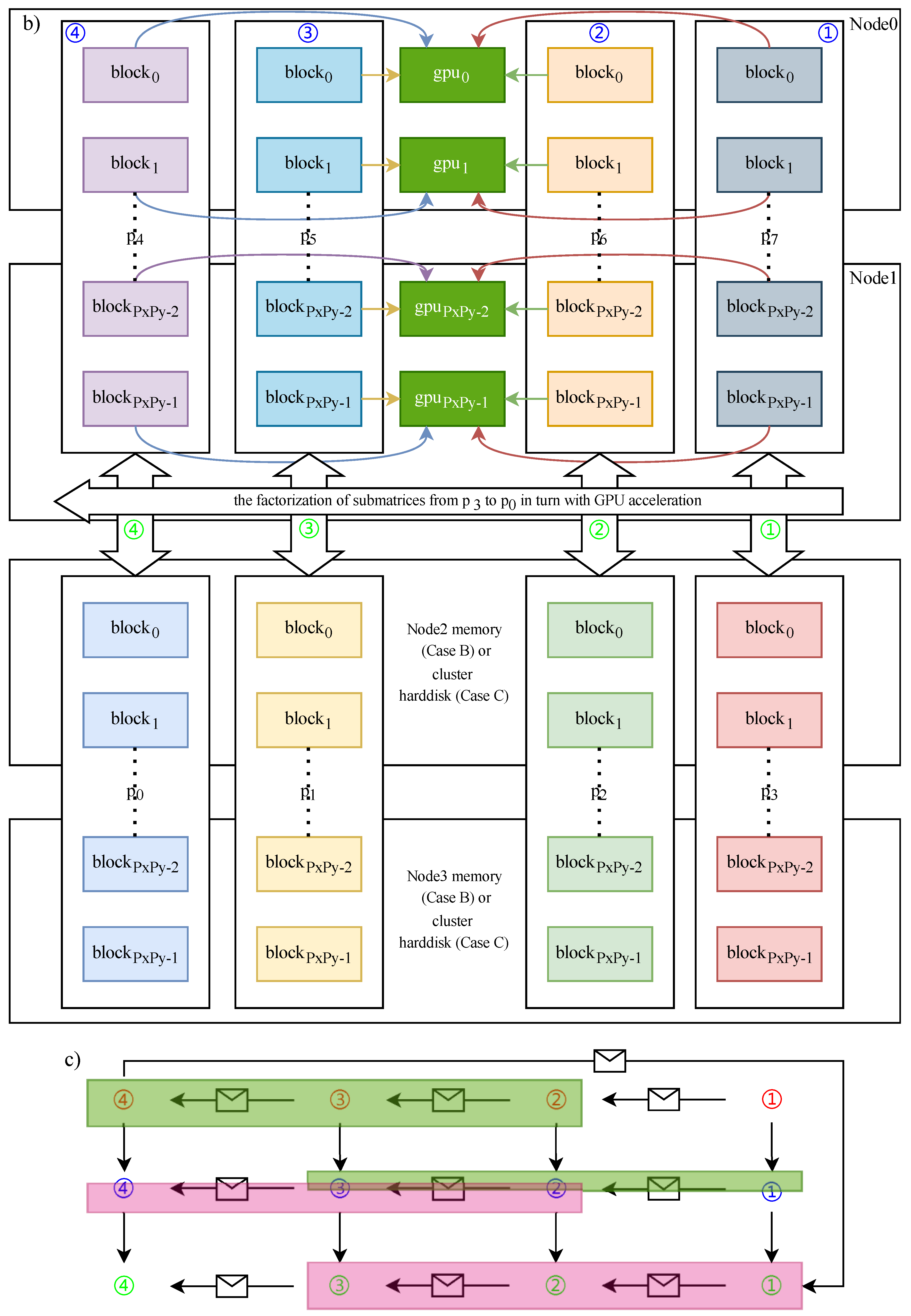
In this case, all the memory of the nodes with GPUs, which include the host memory and all of the GPU device memory, is unable to satisfy the requirement of LU factorization, i.e., i = 1 n M n o d e i < P M i h o s t + M i g p u i = 1 m M n o d e i . The main difference with Case A is that a part of the compute nodes has no GPUs. If we factorize the submatrices in these nodes with GPU acceleration, we must exchange the LU factors data of the compute node without GPU with the compute node with GPU. In addition, we can hide the data exchange behind the LU factorization of the other submatrix with GPU calculation. Taking eight submatrices instead of four as an example, the compute nodes (Node 2 and Node 3) of the last four submatrices do not have GPU (Figure 6a). At the lowest level, i.e., lvl = l, the SuperLU3D_Alternate algorithm of Case B is described as follows:
I.
p 7 exchanges the LU factors with p 3 ( in Figure 6a,c). By now, the LU factors of p 7 are in g r i d 3 and the LU factors of p 3 are in g r i d 0 . Then, we initialize GPU in Node 1 and 2 and factorize p 7 with GPU acceleration ( in Figure 6b,c), while we exchange the other submatrices’ data independently (②→③→④ in Figure 6a,c) until the exchange of p 4 and p 0 is finished. The LU factors of p 4 ~ 7 are in g r i d 0 ~ 3 and the LU factors of p 0 ~ 3 are in g r i d 4 ~ 7 ;
II.
After the LU factorization of p 7 is finished in g r i d 3 , we synchronize the LU factors from GPU to M g p u 2 h o s t 0 7 ~ M g p u 2 h o s t P x P y 1 7 , which are in g r i d 3 , to prepare for the next level, and free the GPU memory occupied by the LU factors ( in Figure 6a,c);
III.
We factorize p 6 , p 5 , and p 4 with GPU acceleration and synchronize the LU factors from GPU to M g p u 2 h o s t 0 i ~ M g p u 2 h o s t P x P y 1 i i = 4,5 , 6 in turn (②→③→④ in Figure 6b,c). At this moment, M g p u 2 h o s t 0 4 ~ 7 ~ M g p u 2 h o s t P x P y 1 4 ~ 7 are in g r i d 0 ~ 3 ;
IV.
The first four submatrices and the last four submatrices exchange data including M g p u 2 h o s t 0 i ~ M g p u 2 h o s t P x P y 1 i and LU factors again in turn after finishing the LU factorization (①→②→③→④ in Figure 6b,c). The LU factors of p 0 ~ 3 are in g r i d 0 ~ 3 and the LU factors of p 4 ~ 7 are in g r i d 4 ~ 7 . M g p u 2 h o s t 0 0 ~ 3 ~ M g p u 2 h o s t P x P y 1 0 ~ 3 are in g r i d 0 ~ 3 and M g p u 2 h o s t 0 4 ~ 7 ~ M g p u 2 h o s t P x P y 1 4 ~ 7 are in g r i d 4 ~ 7 ;
V.
After we factorize the first four submatrices following the same procedures as Case A, we reduce all the common ancestor nodes to finish the LU factorization of the lowest level;
VI.
At the next level l-1, according to the step IV of Case A, submatrix p 0 , p 1 , p 2 , and p 3 are active. We treat the remaining levels in a similar way to Case A. M g p u 2 h o s t 0 4 ~ 7 ~ M g p u 2 h o s t P x P y 1 4 ~ 7 are kept in the host memory for Ancestor_Reduction() in the rest of levels.
The process blocks with the same color in Figure 6c can be performed at the same time to hide the data exchange behind the LU factorization of other submatrices with GPU calculation. In addition, the memory size of the i-th compute node meets n p i M i h o s t + M i g p u < M n o d e i .

2.2.3. Case C: Insufficient Memory for the Entire Cluster

As the size of the matrix increases further, the memory required by the LU factorization is larger than the total memory of the cluster, i.e., P M i h o s t + M i g p u > i = 1 m M n o d e i . Therefore, we have to save part of the intermediate data on the hard disk instead of the cluster memory. In addition, Case C is basically the same as Case B. In this case, we can use the large-capacity, inexpensive, and fast SSD (Solid State Drive), especially NVMe SSD, to improve the speed of data read and write.

3. Time Complexity and Space Complexity

3.1. Time Complexity

To evaluate the computational efficiency of LU factorization using the SuperLU3D algorithm, we consider four different solutions, some with CPU and GPU and some without. The first solution, called “SuperLU3D (CPU)”, involves factorizing each submatrix without GPU acceleration. The second solution, called “SuperLU3D (GPU)”, factorizes each submatrix using GPU acceleration. The third solution, called “SuperLU3D (CPU + GPU)”, is a combination of the first two solutions, where some submatrices are factorized with GPU acceleration, and others without. The fourth solution, which is similar to the SuperLU3D_Alternate algorithm, involves alternating the factorization of each submatrix with GPU acceleration. In this section, we will analyze and compare the time complexity of these four solutions.
During LU factorization, the elapsed time at level-lvl is primarily composed of the time for LU factorization of submatrix-i, denoted as T l v l , i , and the time of the ancestor-reduction step, denoted as T a n c l v l . We define the elapsed time for LU factorization without and with GPU acceleration of submatrix-i as T c p u l v l , i and T g p u l v l , i , respectively. Correspondingly, the elapsed time of all submatrices at level-lvl are T c p u l v l , 0 i P z l v l 1 m a x and T g p u l v l , 0 i P z l v l 1 m a x . In addition, we denote the elapsed time of the data exchange between different processes as T p 2 p l v l in the host memory (like , , , and , , , in Figure 6), and denote the elapsed time of the data exchange between device memory and host memory or hard disk as T g p u 2 h o s t l v l . The sum of T p 2 p l v l and T g p u 2 h o s t l v l is T e x c l v l . In Case A, T e x c l v l = 0 . In the following experiments, we assume that one GPU card can only accelerate one submatrix. In addition, if there is only one submatrix left, we can factorize this submatrix with GPU acceleration completely. We further assume level- l as a conversion marker layer. If l 2 and P z l 1 , P z l 1 = 1 . Therefore, there is one matrix left at level-(l’-1). After level- l , the elapsed time of the SuperLU3D (GPU), SuperLU3D (CPU + GPU), and SuperLU3D_Alternate algorithm is consistent. Based on these settings, we obtained the following results:
SuperLU3D (CPU):
T 0 = l v l = 0 l T c p u l v l , 0 i P z l v l 1 m a x + T a n c l v l
SuperLU3D (GPU):
T 1 = l v l = 0 l T g p u l v l , 0 i P z l v l 1 m a x + T a n c l v l
SuperLU3D (CPU + GPU):
T 2 = l v l = l l T l v l , 0 i P z l v l 1 m a x + T a n c l v l + l v l = 0 l 1 T g p u l v l , 0 + T a n c l v l
SuperLU3D_Alternate:
T 3 = l v l = l l T e x c l v l + i = 0 P z l v l 1 T g p u l v l , i + T a n c l v l + l v l = 0 l 1 T g p u l v l , 0 + T a n c l v l
The larger the matrix size, the more obvious effect of the GPU acceleration for matrix multiplication. Thus, when we factorize the very large matrix, there are two inequalities as follows:
T g p u l v l , 0 i P z l v l 1 m a x < T c p u l v l , 0 i P z l v l 1 m a x ;
T g p u l v l , 0 i P z l v l 1 m a x < i = 0 P z l v l 1 T g p u l v l , i ;
T l v l , 0 i P z l v l 1 m a x = T c p u l v l , 0 i P z l v l 1 m a x , f o r   T 2 T g p u l v l , 0 i P z l v l 1 m a x ,   f o r   T 1 .
By comparing Equations (6)–(9), the same part of elapsed time is l v l = 0 l T a n c l v l . After excluding l v l = 0 l T a n c l v l , we compare Equations (6)–(9) to find that T 1 is the least time-consuming solution, and T 2 < T 0 .
In summary, the optimal algorithm is SuperLU3D (GPU). However, if the GPU memory is not enough to accelerate the LU factorization of all submatrices, we will select the other three solutions instead. Because T 2 < T 0 , and the relationship between T 2 and T 3 is unknown, we will focus on the simplified minimum of T = T 2 T 3 , denoted as T m i n , in theory, and its influencing factors.
From Equations (8) and (9),
T = T 2 T 3 = l v l = l l T c p u l v l , 0 i P z l v l 1 m a x T e x c l v l i = 0 P z l v l 1 T g p u l v l , i
We assume the speed-up ratio of i-th submatrix at level-lvl to be f = T c p u l v l , i T g p u l v l , i . Through the LU factorization of the test matrices in the numerical experiments, we discover that the speed-up ratio at level-l is the smallest, i.e.,
f m i n = T c p u l , 0 i P z l 1 m a x T g p u l , 0 i P z l 1 m a x
From Equations (10) and (14),
T c p u l v l , 0 i P z l v l 1 m a x = f T g p u l v l , 0 i P z l v l 1 m a x f m i n T g p u l v l , 0 i P z l v l 1 a v g = f m i n i = 0 P z l v l 1 T g p u l v l , i P z l v l ,
where the average of T g p u l v l , 0 i P z l v l 1 is
T g p u l v l , 0 i P z l v l 1 a v g = i = 0 P z l v l 1 T g p u l v l , i P z l v l .
Combining Equations (13) and (15), the simplified minimum of T is
T m i n = l v l = l l f m i n P z l v l 1 i = 0 P z l v l 1 T g p u l v l , i T e x c l v l
From Equation (17), we consider that T m i n is affected by P z l v l and T e x c l . And the per-process memory of LU factors in SuperLU3D algorithm is approximately equal to n P z × P x y log n [4]. Therefore, T e x c l has positive correlation with n, and has negative correlation with P z . In addition, the GPU acceleration can improve the performance by 1.4–3.5× as compared to the SuperLU3D algorithm without GPU acceleration [4]. In conclusion, P z is the primary factor affecting the performance of the SuperLU3D_Alternate algorithm, and the secondary factor is n. While alternating LU factorization seems to reduce parallelism, it can solve the very large matrix factorization problem with limited GPU resources. Moreover, in the case of GPU acceleration, choosing the appropriate P z is still possible to make T m i n > 0 or T > 0 .

3.2. Space Complexity

The host memory ( M h o s t ) and device memory ( M d e v ) of all the LU factors for the four solutions mentioned in Section 3.1 are given by the following expressions:
SuperLU3D (CPU):
M h o s t ( 0 ) = i = 0 P z l 1 M i h o s t ,   M d e v ( 0 ) = 0 ;
SuperLU3D (GPU):
M h o s t ( 1 ) = i = 0 P z l 1 M i h o s t ,   M d e v ( 1 ) = i = 0 P z l P x P y 1 M i g p u ;
SuperLU3D (CPU + GPU):
M h o s t ( 2 ) = i = 0 P z l 1 M i h o s t ,   M d e v ( 2 ) = i = 0 P x P y 1 M i g p u ;
SuperLU3D_Alternate:
M h o s t 3 = i = 0 P z l 1 ( M i h o s t + M d e v 2 h o s t ) ,   M d e v ( 3 ) = i = 0 P x P y 1 M i g p u ;
where M i h o s t is the per-process memory, M i g p u is the per-process GPU memory, and M d e v 2 h o s t is the per-process host memory synchronized with GPU. From the above formulas, we can obtain M i h o s t = M i g p u = M d e v 2 h o s t .
Comparing Equations (18)–(21), we further obtain that
M h o s t 0 = M h o s t 1 = M h o s t 2 = 0.5 M h o s t 3 ,
M d e v ( 1 ) = P z l M d e v ( 2 ) = P z l M d e v ( 3 ) .
The host memory required by the SuperLU3D_Alternate algorithm is twice that of the SuperLU3D algorithm, which is primarily due to the need to synchronize matrices L and U from the GPU memory in the intermediate processes. Conversely, the GPU memory required by the SuperLU3D_Alternate algorithm is only 1 / P z l that of the SuperLU3D algorithm. Therefore, SuperLU3D_Alternate is able to utilize limited GPU to factorize larger scale matrices than SuperLU3D.
Because the MPI nonblocking communications occur in step (2) and (4) in Section 2.1.2, at level-l, there is only one submatrix performing LU factorization for the SuperLU3D_Alternate algorithm, but there are P z l submatrices performing LU factorization in parallel for the SuperLU_DIST algorithm. Therefore, the amount of data in the MPI nonblocking communication of SuperLU3D_Alternate is 1 / P z l that of SuperLU3D algorithm.

4. Numerical Experiments and Results

Given a very large matrix, if the host memory satisfies the computational requirements but the GPU memory does not, there are three possible solutions: SuperLU3D (CPU), SuperLU3D (CPU + GPU), and SuperLU3D_Alternate, as discussed in Section 3.1. To evaluate the performance of the SuperLU3D_Alternate algorithm, we compared the elapsed times of these three solutions. Additionally, we calculated T for test matrices in both Case A and Case B to confirm the accuracy of T m i n as mentioned in Section 3.1.
As the matrix size increases, the host memory on the cluster may not be sufficient to meet the computational requirements. Alternatively, the amount of nonblocking communication data between different processes may exceed the limit of the cluster communication buffer, leading to system memory overflow. In such situations, the SuperLU3D_Alternate algorithm is recommended.

4.1. Setup

For SuperLU3D (CPU), we combined one “AMD-server” node and three “GPU-server” nodes in a hybrid cluster. The specific configurations are shown in Table 2.
For SuperLU3D (CPU + GPU) and SuperLU3D_Alternate, we used multi-GPU on three “GPU-server” nodes. The GPU node configuration is shown in Table 2. We ensured that a graphics card was only used by one process. In particular, for the SuperLU3D_Alternate algorithm, while we performed LU factorization with GPU acceleration on the “GPU-server” node, a part of the LU factors was also stored in the “AMD-server” node and “Intel-server” node without any computational task. We tested this algorithm via the mixed use of multiple types of servers.

4.2. Test Matrices

We took 11 matrices from a number of numerical problems of two-dimensional (such as G3_circuit) and three-dimensional PDEs (such as nlpkkt80) for testing the SuperLU3D_Alternate algorithm (Table 3). The last four matrices (geodynamics1~4) in Table 3 were obtained from the finite difference numerical simulation problem of geodynamics based on the 3D Stokes equations and the incompressible mass continuity equations. The LU factorization of these four matrices consumes large amounts of host memory and device memory. Therefore, these matrices are very suitable for testing our algorithms. As can be seen from Table 3, the scale of computing from CoupCons3D to geodynamics4 increases sequentially.

4.3. Comparison of Results

The numerical experiments set P x = 2 , P y = 3 , P z = 2 , and n s = 100 , i.e., the total number of processes was 12, and all the matrices were divided into two submatrices. We ran 12 MPI processes on the cluster, and each MPI process used four OpenMP threads. The number of GPUs involved in the calculation was six, which is half the number of processes, i.e., only half the processes were permitted to invoke GPU.
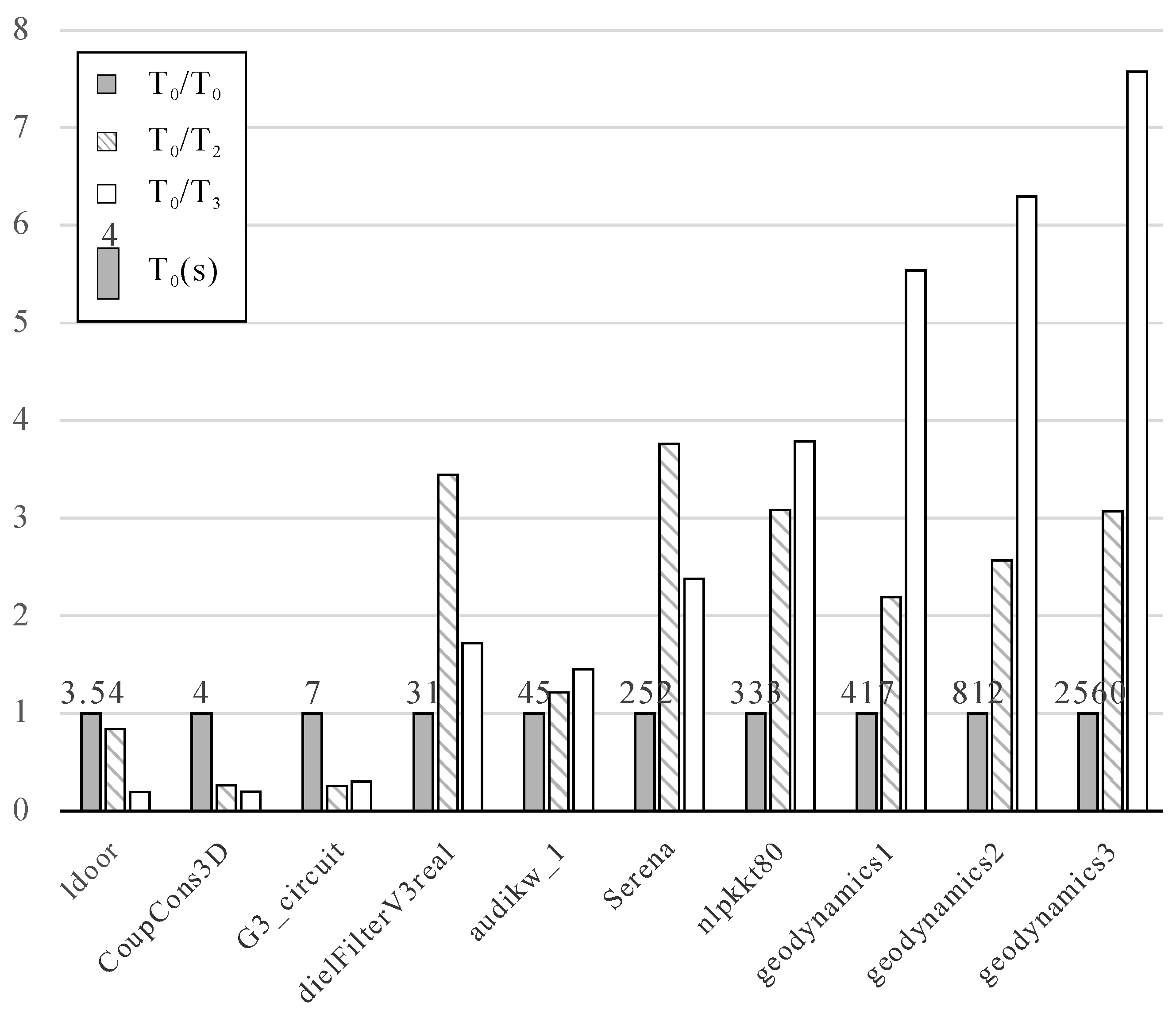
We obtained the elapsed times and speed-up ratios of 11 matrices in Case A (Table 4). “geodynamics4” was unable to be factorized by the SuperLU3D algorithm on the cluster because of the large amount of nonblocking communication data. The bar graph based on the speed-up ratios, including T 2 / T 0 and T 3 / T 0 , is shown in Figure 7. The results of T 0 show that the elapsed time of SuperLU3D (CPU) increased with increasing matrix size. In comparison with T 2 / T 0 and T 3 / T 0 , SuperLU3D_Alternate achieved a speed of up to 8× that of SuperLU3D (CPU) and 2.5× that of SuperLU3D (CPU + GPU) on the hybrid cluster with six Tesla V100S GPUs. The SuperLU3D_Alternate algorithm was proved to be more efficient than SuperLU3D (CPU + GPU) under the same device memory consumption in our experiments. This was thanks to the fact that the LU factorization of each submatrix was able to take advantage of GPU acceleration. It is worth mentioning that, due to the increasing amount of nonblocking communication data, the SuperLU3D algorithm will be unstable or even break in running programs.
In addition, in the numerical experiments using SuperLU3D (CPU) and SuperLU3D (CPU + GPU), there was a certain probability that “geodynamics3” failed in factorization, while “geodynamics4” was not always successful. Therefore, the SuperLU3D_Alternate algorithm is more applicable for very large sparse matrices than SuperLU3D (CPU) and SuperLU3D (CPU + GPU).
Finally, we conducted experiments on Case C using data from geodynamics1, geodynamics2, and geodynamics3. All these submatrices, which were created during LU factorization, were initially stored on the hard drive, and each one was sequentially read into the memory for computation to reduce the memory requirements of very large sparse LU factorization. The times spent on the LU factorization of these three matrices were 1881 s, 3290 s, and 4988 s, respectively. In addition, the memory consumption of these matrices in Case C was about 60% of that in Case A.

4.4. Correctness of Time Complexity Analysis

In the second experiment, we compared the elapsed times of the SuperLU3D_Alternate and SuperLU3D (CPU + GPU) algorithms under Case A and Case B. The biggest difference from Case A was that the compute nodes on which a part of processes reside had no GPUs in Case B. Therefore, we needed to invoke GPUs across other nodes, resulting in increasing the time spent on data exchange ( T e x c ). We obtained T and T m i n of the test matrices, including geodynamics1, geodynamics2, and geodynamics3 (Table 5), in Case A and Case B, where T = T 2 T 3 , and T m i n is the simplified minimum of T . In Table 5, all the results of T are bigger than T m i n . These results verify the analysis of T and T m i n in Section 3.1. Therefore, when we choose a small P z in the SuperLU3D_Alternate algorithm, we can ensure that T > 0 . In addition, the results of T > 0 show that, even if the submatrix needs to be decomposed alternately and additional data need to be exchanged at each level, SuperLU3D_Alternate with GPU acceleration has better computational efficiency than SuperLU3D (CPU + GPU).

5. Conclusions and Future Work

The SuperLU3D_Alternate algorithm described in this paper is suitable for solving the problem of LU factorization for large sparse matrices by utilizing hardware resources of different scales, even in situations where there may be insufficient memory available. This includes cases where there is sufficient memory available on GPU nodes, cases where there is insufficient memory available on GPU nodes, and cases where there is insufficient memory available across the entire cluster. Results from numerical experiments demonstrate that this approach is not only feasible but also improves computational efficiency with the help of GPU acceleration compared to SuperLU3D (CPU) and SuperLU3D (CPU + GPU).
(1) In Table 3, we compared the LU factorization of test matrices using SuperLU3D (CPU), SuperLU3D (CPU + GPU), and SuperLU3D_Alternate. The results indicate that, as the SuperLU3D (CPU) algorithm takes longer, the SuperLU3D_Alternate algorithm becomes more efficient than SuperLU3D (CPU + GPU) while consuming the same GPU memory. The numerical experiments showed that, on a hybrid cluster with six Tesla V100S GPUs, SuperLU3D_Alternate achieved speeds of up to 8× that of SuperLU3D (CPU) and 2.5× that of SuperLU3D (CPU + GPU).
(2) The SuperLU3D_Alternate algorithm proposed in this study offers a solution to the problem of LU factorization for very large matrices when the GPU memory is insufficient. By dividing the matrix into submatrices and performing LU factorization alternately with GPU acceleration, the algorithm allows for the utilization of the cluster’s host memory or hard disk to store intermediate LU factors of submatrices. This approach enables the efficient processing of very large matrices.
(3) The SuperLU3D_Alternate algorithm reduces the amount of data exchange required, which prevents it from exceeding the limit of the cluster MPI nonblocking communication buffer. This, in turn, enhances the stability of the algorithm.
In the current work, we observed that the SuperLU3D_Alternate algorithm requires additional synchronization of GPU data transmission between different GPUs with the host memory, which can result in increased latency and reduced throughput. Therefore, direct communication between GPUs can improve the overall performance and efficiency of the algorithm. NVIDIA GPUDirect technologies can provide low-latency, high-bandwidth communication between NVIDIA GPUs. Therefore, future work will focus on optimizing interprocess communication efficiency using technologies such as GPUDirect RDMA [21].

Author Contributions

Writing—original draft, J.C.; writing—review & editing, P.Z. All authors have read and agreed to the published version of the manuscript.

Funding

This work is sponsored by National Natural Science Foundation of China [41774145] and the Pre-research Project on Civil Aerospace Technologies [D020101] of CNSA.

Data Availability Statement

All the relevant data presented in this study are available from the corresponding author upon reasonable request.

Conflicts of Interest

The authors declare no conflict of interest.

References

  1. Amestoy, P.R.; Guermouche, A.; L’Excellent, J.Y.; Pralet, S. Hybrid scheduling for the parallel solution of linear systems. Parallel Comput. 2006, 32, 136–156. [Google Scholar] [CrossRef] [Green Version]
  2. Amestoy, P.R.; Duff, I.S.; L’Excellent, J.Y.; Koster, J. A fully asynchronous multifrontal solver using distributed dynamic scheduling. SIAM J. Matrix Anal. Appl. 2001, 23, 15–41. [Google Scholar] [CrossRef] [Green Version]
  3. Schenk, O.; Gartner, K. On fast factorization pivoting methods for sparse symmetric indefinite systems. Electron. Trans. Numer. Anal. 2006, 23, 158–179. [Google Scholar]
  4. Sao, P.Y.; Li, X.Y.S.; Vuduc, R. A communication-avoiding 3D algorithm for sparse LU factorization on heterogeneous systems. J. Parallel Distrib. Comput. 2019, 131, 218–234. [Google Scholar] [CrossRef]
  5. Sao, P.Y.; Vuduc, R.; Li, X.Y.S. A distributed CPU-GPU sparse direct solver. In European Conference on Parallel Processing; Springer: Berlin/Heidelberg, Germany, 2014; pp. 487–498. [Google Scholar] [CrossRef]
  6. Li, X.Y.S.; Demmel, J.W. SuperLU_DIST: A scalable distributed-memory sparse direct solver for unsymmetric linear systems. ACM Trans. Math. Softw. 2003, 29, 110–140. [Google Scholar] [CrossRef]
  7. Demmel, J.W.; Eisenstat, S.C.; Gilbert, J.R.; Li, X.S.; Liu, J.W.H. A supernodal approach to sparse partial pivoting. SIAM J. Matrix Anal. Appl. 1999, 20, 720–755. [Google Scholar] [CrossRef]
  8. Abhyankar, S.; Brown, J.; Constantinescu, E.M.; Ghosh, D.; Smith, B.F.; Zhang, H. PETSc/TS: A modern scalable ODE/DAE solver library. arXiv 2018. [Google Scholar] [CrossRef]
  9. Heroux, M.A.; Bartlett, R.A.; Howle, V.E.; Hoekstra, R.J.; Hu, J.J.; Kolda, T.G.; Lehoucq, R.B.; Long, K.R.; Pawlowski, R.P.; Phipps, E.T.; et al. An overview of the Trilinos Project. ACM Trans. Math. Softw. 2005, 31, 397–423. [Google Scholar] [CrossRef] [Green Version]
  10. Falgout, R.D.; Jones, J.E.; Yang, U.M. Conceptual interfaces in HYPRE. Future Gener Comp Syst. 2006, 22, 239–251. [Google Scholar] [CrossRef]
  11. Chen, L.; Song, X.; Gerya, T.V.; Xu, T.; Chen, Y. Crustal melting beneath orogenic plateaus: Insights from 3-D thermo-mechanical modeling. Tectonophysics 2019, 761, 1–15. [Google Scholar] [CrossRef]
  12. Chen, L.; Capitanio, F.A.; Liu, L.; Gerya, T.V. Crustal rheology controls on the Tibetan plateau formation during India-Asia convergence. Nat. Commun. 2017, 8, 15992. [Google Scholar] [CrossRef] [PubMed] [Green Version]
  13. Chen, L.; Gerya, T.V. The role of lateral lithospheric strength heterogeneities in orogenic plateau growth: Insights from 3-D thermo-mechanical modeling. J. Geophys. Res. Solid Earth 2016, 121, 3118–3138. [Google Scholar] [CrossRef] [Green Version]
  14. Li, Z.-H.; Xu, Z.; Gerya, T.; Burg, J.-P. Collision of continental corner from 3-D numerical modeling. Earth Planet. Sci. Lett. 2013, 380, 98–111. [Google Scholar] [CrossRef]
  15. Gaihre, A.; Li, X.S.; Liu, H. GSOFA: Scalable sparse symbolic LU factorization on GPUs. IEEE Trans. Parallel Distrib. Syst. 2021, 33, 1015–1026. [Google Scholar] [CrossRef]
  16. Duff, I.S. The impact of high-performance computing in the solution of linear systems: Trends and problems. J. Comput. Appl. Math. 2000, 123, 515–530. [Google Scholar] [CrossRef] [Green Version]
  17. Li, X.S.; Demmel, J.W. Making sparse Gaussian elimination scalable by static pivoting. In Proceedings of the 1998 ACM/IEEE Conference on Supercomputing, Orlando, FL, USA, 7–13 November 1998; p. 34. [Google Scholar] [CrossRef] [Green Version]
  18. Li, X.Y.S.; Demmel, J.W.; John, R.G.; Laura, G.; Piyush, S.; Meiyue, S.; Ichitaro, Y. SuperLU Users’ Guide; University of California: Berkeley, CA, USA, 2018. [Google Scholar]
  19. Davis, T.A.; Hu, Y.F. The University of Florida sparse matrix collection. ACM Trans. Math. Softw. 2011, 38, 1–25. [Google Scholar] [CrossRef]
  20. Gerya, T.V. Introduction to Numerical Geodynamic Modelling, 2nd ed.; Cambridge University Press: Cambridge, UK, 2019. [Google Scholar]
  21. Potluri, S.; Hamidouche, K.; Venkatesh, A.; Bureddy, D.; Panda, D.K. Efficient inter-node MPI communication using GPUDirect RDMA for InfiniBand clusters with NVIDIA GPUs. In Proceedings of the 2013 42nd International Conference on Parallel Processing, Lyon, France, 1–4 October 2013; pp. 80–89. [Google Scholar] [CrossRef]
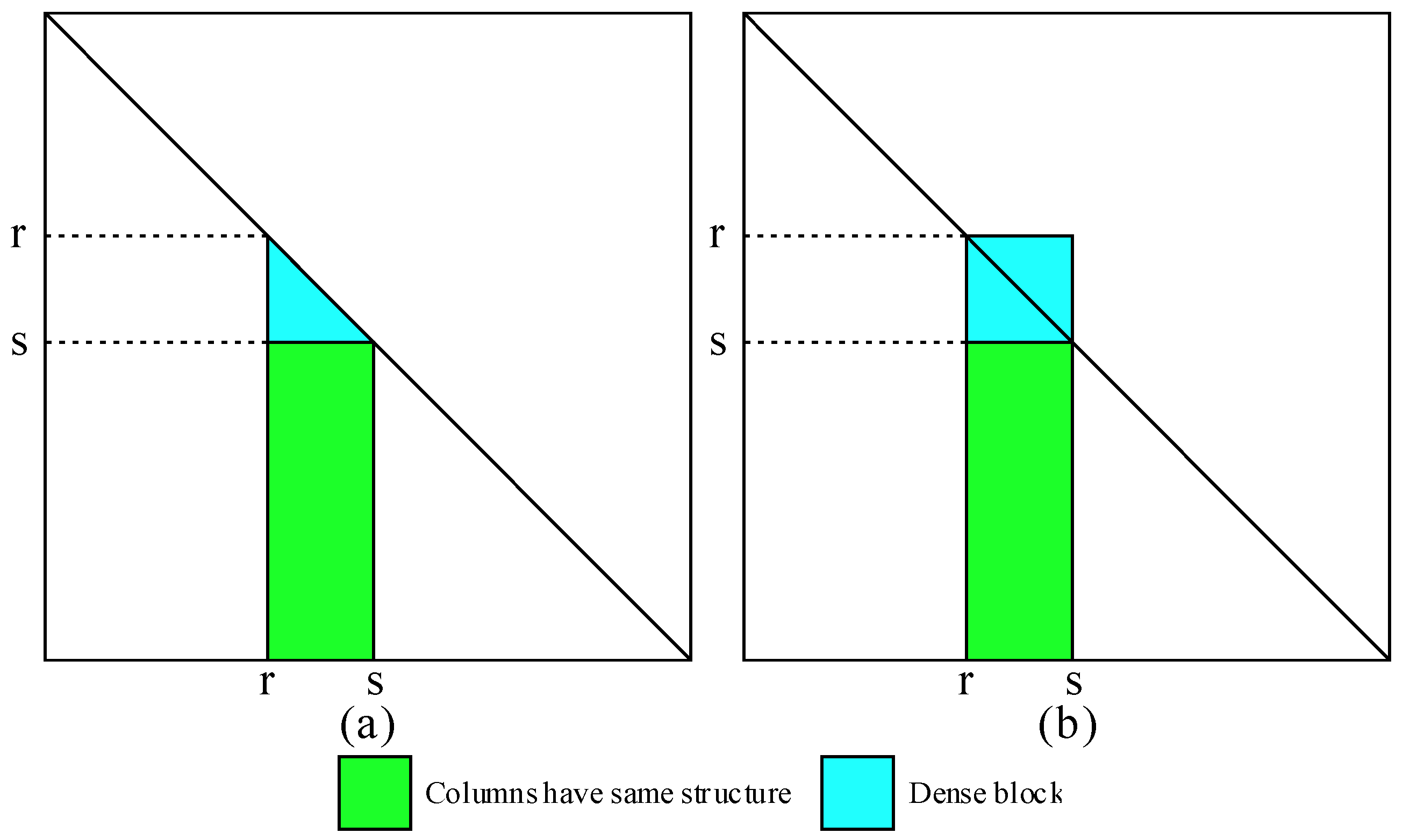
Figure 1. Definition of supernodes in the SuperLU_DIST algorithm (modified from [7]). A supernode is a set of consecutive columns of matrix L with a dense triangular block below the diagonal and with the same nonzero structure below the triangular block [15]. (a) A supernode without full diagonal block in U; (b) a supernode with full diagonal block in U. Definition (a,b) state that for a supernode that already contains columns r through s − 1, two requirements are needed for the next column s to be included in this supernode: (i) The number of nonzeros in column s of L shall be one fewer than that of column s − 1; (ii) there shall be a nonzero at (r,s) in the filled matrix U. If either of the requirements is not met, column s will not belong to the supernode. Supernode (a) needs to meet requirement (i), and supernode (b) needs to meet requirement (i) + (ii).
Mathematics 11 03149 g001
Figure 2. The elimination tree of matrix A. The circle with number i denotes the i-th tree node. According to the construction principle of the elimination tree, it is concluded that columns 1, 2, and 3 correspond to the leaf nodes 1, 2, and 3 in the elimination tree. Similarly, node 5 is also a leaf node. In the lower triangular matrix, a 42 and a 43 are the first nonzero elements of their column, and we set the edges E42 and E43 between node 4 and node 2, node 4 and node 3, respectively. Similarly, the first nonzero elements in column 6 are a 61 , a 64 , and a 65 . We set the edges E61, E64, and E65 between node 6 and node 1, node 6 and node 4, node 6 and node 5. And thus, we obtain the elimination tree corresponding to the sparse matrix A.
Mathematics 11 03149 g002
Figure 3. The factorization procedure of the k-th supernode in the 2D process grid. Let a matrix with eight supernodal blocks be distributed in a two-dimensional 2 × 3 block-cyclic fashion, and P x = 2 , P y = 3 . When k = 1, the k-th supernode belongs to the process P k , k = 4 . We define that P i , j = m o d i , P x × P y + m o d j , P y . Firstly, process 4 factorizes A 11 into L 11 U 11 . Secondly, process 4 broadcasts L 11 across its process row P { 1 , : } to block A 1 , : (the blue horizontal arrow) and U 11 across its process column P { : , 1 } to block A : , 1 (the blue vertical arrow). Processes 3 and 5 in process row P { 1 , : } receive block L 11 , and process 1 in process column P { : , 1 } receives block U 11 .Thirdly, processes 3, 4, and 5 in P { 1 , : } calculate U 1 , : = L 11 1 A 1 , : , and convert the U 1 , : into a dense matrix U ~ 1 , : . Processes 1 and 4 in P { : , 1 } calculate L : , 1 = A : , 1 U 11 1 . Fourthly, processes 3, 4, and 5 in P { 1 , : } broadcast blocks of U ~ 1 , : to processes 0, 1, and 2 in P : , 2 : 5 , respectively. Process 1 in P { : , 1 } broadcasts blocks of L : , 1 to process 0 in P { 2 : 5 , : } , and process 3 in P { : , 1 } broadcasts blocks of L : , 1 to process 2 in P { 2 : 5 , : } . Finally, we use dense matrix blocks to compute V = L i k U ~ k j and update A i j by A i j = A i j L i k U ~ k j in the process P i , j .
Mathematics 11 03149 g003
Figure 4. A matrix is divided into four submatrices (processes) p 0 ~ p 3 according to a two-layer partition of the elimination tree (a), and each submatrix is mapped to a 2D process grid (b) (modified from [4]). We index subtrees in the top-down order from node-0 to node-6. We define P z ( l v l ) = 2 l v l as the number of submatrices at the lvl-th level, i.e., P z ( 2 ) = 4 ,   P z ( 1 ) = 2 and P z ( 0 ) = 1 . The i-th submatrix is factorized in g r i d i . The processes at the same relative position in different 2D process grids are allowed to communicate (arrows in (b)).
Mathematics 11 03149 g004
Figure 5. The flow diagram (a) and sequence diagram (b) of Case A. The matrix is divided into four submatrices denoted as p 0 , p 1 , p 2 , and p 3 . The circle with the number i denotes the i-th order of the factoration at the l-th level. The i-th submatrix is factorized in g r i d i with P x × P y processes (Figure 4b) in Compute Node 0 and Node 1. Function InitSparseLU2D_GPU(), copyLU2D_GPU2CPU(), and copyLU2D_CPU2GPU() of (b) are shown in Algorithm 1.
Mathematics 11 03149 g005
Figure 6. The flow diagram of Case B and Case C. The matrix is divided into eight submatrices denoted as p 0 ~ p 7 . p 0 ~ p 3 are stored in Compute Node 0 and Node 1, while p 4 ~ p 7 are stored in Compute Node 2 and Node 3 (or the hard disk). (a,b) The two successive steps of Case B and Case C. (c) The MPI message transfer process between 2D process grids. Red circled number: two processes with the same m o d p i d , P x y exchange the LU factors with each other. Blue circled number: initialize GPU→LU factorization with GPU acceleration→copy the LU factors from GPU to M g p u 2 h o s t 0 i ~ M g p u 2 h o s t P x P y 1 i →free GPU memory. Green circled number: two processes exchange data including the LU factors and M g p u 2 h o s t 0 i ~ M g p u 2 h o s t P x P y 1 i  with each other again; Mathematics 11 03149 i001: task end signal. If the other 2D process grid receives this signal, it will start its task at once.
Mathematics 11 03149 g006aMathematics 11 03149 g006b
Figure 7. The speed-up ratios of the SuperLU3D (CPU + GPU) and SuperLU3D_Alternate algorithms as compared with the SuperLU3D (CPU) algorithm in Case A. T 0 , T 1 , T 2 , and T 3 are mentioned in Table 4. The numbers on the top of the gray bars are the elapsed time of the SuperLU3D (CPU) algorithm. From this figure, we can see that the advantage of the SuperLU3D_Alternate algorithm over the SuperLU3D (CPU) and SuperLU3D (CPU + GPU) algorithms becomes more obvious as the sizes of test matrices increases.
Mathematics 11 03149 g007
Table 1. List of symbols mentioned.
SymbolDescription
Pnumber of MPI processes
P x , P y , P z 3D process grid dimensions
P x y number of processes in xy plane
P { k , : } groups of processes assigned to the k-th supernodal row
P { i : j , : } i~j-th group of processes assigned to the k-th supernodal row (i < j)
P { : , k } groups of processes assigned to the k-th supernodal column
P { : , i : j } i~j-th groups of processes assigned to the k-th supernodal column (i < j)
P i , j No. m o d i , P x × P y + m o d j , P y process
pidprocess ID
p i the i-th submatrix
g r i d i the i-th 2D process grid
ndimension of a matrix
nnzthe number of nonzero elements in a matrix
Eelimination tree
llevel of elimination tree ( l = log 2 P z )
mnumber of compute nodes in the cluster
M n o d e i memory size of the i-th compute node
M g p u GPU DRAM
n p i number of processes of the i-th node
k i number of GPU of the i-th node
G P U n o d e n u m number of nodes with GPU ( k i > 0 )
P z l v l number of submatrices at lvl-th level
M i h o s t M n o d e i memory occupied by LU factors per process
M i g p u M g p u GPU memory occupied by LU factors per process
M d e v 2 h o s t host memory copied from GPU per process
M g 2 h j i host memory of j-th process in g r i d i copied from j-th GPU
grid3d.commthe 3D MPI communicator
Table 2. Cluster specification.
ParameterGPU-ServerIntel-ServerAMD-Server
CPU2 × Intel(R) Xeon(R) Gold 6226R CPU @ 2.90 GHz2 × Intel(R) Xeon(R) Silver 4110 CPU @ 2.10 GHz2 × AMD EPYC 7742 @2.25 GHz
Memory256 GB256 GB512 GB
GPUs per node200
Type of GPUTesla V100S “Volta”----
GPU DRAM32 GB HMB2----
CUDA Cores per GPU5120----
NVMe SSD4 TB4 TB4 TB
InfiniBand Bandwidth2.5 Gb/s2.5 Gb/s2.5 Gb/s
Operating systemCentOS Linux release 7.4.1708
CompilerNVIDIA HPC-X
LibrariesCUDA 10.2, Intel MKL
Table 3. Eleven matrices for testing LU solvers.
Namen annz annz/nApplication
CoupCons3D b4.2 × 1051.7 × 10741.5Structural Problem
Ldoor b9.5 × 1054.2 × 10744.6Structural Problem
Seren b1.4 × 1066.4 × 10746.1Structural Problem
audikw_1 b9.4 × 1057.8 × 10782.0Structural Problem
dielFilterV3real b1.1 × 1068.9 × 10781.0FEM/EM
G3_circuit b1.6 × 1067.7 × 1064.8Circuit Sim.
nlpkkt80 b1.1 × 1062.8 × 10726.5KKT matrices
geodynamics1 c3.3 × 1064.5 × 10714.0FDM 3D d
geodynamics2 c4.5 × 1066.3 × 10714.0FDM 3D d
geodynamics3 c5.1 × 1067.1 × 10714.0FDM 3D d
geodynamics4 c5.4 × 1067.5 × 10714.0FDM 3D d
Notes: a—n is the dimension of the matrix, and nnz is the total number of nonzero elements; b—these matrices were obtained from the University of Florida Sparse Matrix Collection [19]; c—the last four matrices were obtained from the finite difference numerical simulation of geodynamics based on the 3D Stokes equations and the incompressible continuity equations [20]. d—FDM 3D is the abbreviation of 3D finite difference method.
Table 4. The elapsed time and speed-up ratio of the SuperLU3D (CPU + GPU) and SuperLU3D_Alternate algorithms as compared with the SuperLU3D (CPU) algorithm in Case A.
NamePer-Process GPU Memory (GB)SuperLU3D
(CPU)
T 0
(Second)
SuperLU3D
(CPU+GPU)
T 2
(Second)
SuperLU3D_
Alternate
T 3
(Second)
T 0 / T 2 T 0 / T 3
ldoor4.33.544.21180.8408550.196667
CoupCons3D4.3415200.2666670.2
G3_circuit4.5727230.2592590.304348
dielFilterV3real5.0319183.4444441.722222
audikw_16.74537311.2162161.451613
Serena10.8252671063.7611942.377358
nlpkkt8011.8333108883.0833333.784091
geodynamics118.78643941562.1928935.538462
geodynamics230.319327523072.5691496.29316
geodynamics330.325608333383.0732297.573964
geodynamics430.3----896----
Table 5. The elapsed times of the SuperLU3D_Alternate and SuperLU3D (CPU + GPU) algorithms in Case A and Case B.
Name f m i n  a P z T e x c l  b
(Second)
T 2  c
(Second)
T 3  c
(Second)
T  c
(Second)
T m i n  c
(Second)
geodynamics1_case_A4.6320394156238136.92
geodynamics1_case_B4.31262.1139422516954.34
geodynamics2_case_A4.3420752307445247.83
geodynamics2_case_B3.282118.3475246728517.35
geodynamics3_case_A3.6420833338495275.47
geodynamics3_case_B3.372145.7683358624753.08
a—the speed-up ratio at level-l f m i n = T c p u l , 0 i P z l 1 m a x T g p u l , 0 i P z l 1 m a x ; b— T e x c l = T p 2 p l + T g p u 2 h o s t l where T p 2 p l is the elapsed time of the memory data exchange between different processes and T g p u 2 h o s t l is the elapsed time of the data exchange between device memory and host memory or hard disk at level-l; c— T 2 , T 3 , T , and T m i n are mentioned in Table 4. In addiction, T m i n is obtained by Equation (17) with l = 2 and P z = 2 .
Disclaimer/Publisher’s Note: The statements, opinions and data contained in all publications are solely those of the individual author(s) and contributor(s) and not of MDPI and/or the editor(s). MDPI and/or the editor(s) disclaim responsibility for any injury to people or property resulting from any ideas, methods, instructions or products referred to in the content.