Finite-Sized Orbiter’s Motion around the Natural Moons of Planets with Slow-Variable Eccentricity of Their Orbit in ER3BP

Abstract

This article is devoted to the study of the stability of movement of a satellite of finite size around the natural satellites of the planets in the solar system, using the new concept of ER3BP with variable eccentricity. This concept was introduced earlier for the variable spin state of a secondary planet correlated implicitly to the motion of the satellite for its trapped orbit near the secondary planet (which is involved in the Kepler duet “Sun-planet”). But it is of real interest to explore another kind of this problem, plane ER3BP “planet-moon-satellite”. Here, we consider two primary celestial bodies, a planet and a moon, the latter revolves around its common barycenter in a quasi-elliptical orbit in a fixed plane (invariable plane) around the planet with a slowly varying eccentricity on a large time scale due to tidal phenomena. This study presents both new theoretical and numerical results for various cases of the “planet-moon-satellite” trio.

1. Introduction

Equations of the restricted three-body problem R3BP present the dynamical model of motion of a mini-planetoid with a small mass under the governing combined action of Newtonian gravity by two large bodies (called primaries in celestial mechanics), dancing in their mutual celestial motion on Kepler planar orbits around a barycenter. The celestial mechanics community has seen many modern and old studies presenting outstanding results in R3BP (e.g., [1,2,3,4,5,6,7,8,9,10], but not limited to these).

In this work, we will assume that the small finite-sized satellite m is orbiting near the natural moon m_moon of a planet in the solar system with variable eccentricity of the moon in its motion around the planet (the methodological basis describing this kind of motion was considered previously by the authors of reference [8]). So, we consider here two primaries, M_planet and m_moon; the latter is orbiting around their common barycenter in a quasi-elliptic orbit with slow-changing eccentricity (on a large-time scale) due to tidal phenomena. Our aim is to investigate the motion of the small finite-sized satellite around the natural moon of the planet in a quasi-stable elliptic orbit. The relative distances ρ of the positions of primaries are always changing in mutual permanent motion (in the ER3BP) in their elliptical orbits [1]:

$$\rho = \frac{a_p\cdot (1-e^2)}{1+e\cdot \cos f}$$

where, a_p is the semimajor axis of elliptic orbits of primaries around their common centre of mass (here, a scale of distances is chosen so that {a_p (0) × (1 − e(0))} = 1), e is the variable small eccentricity (e << 1) and f is the true anomaly. As formulated by the authors of reference [8], angular motion is given by:

$$\frac{df}{dt} = {\left(\frac{GM}{a_p^3\cdot {(1-e^2)}^3}\right)}^{\frac{1}{2}}\cdot {(1+e\cdot \cos f)}^2$$

(1)

where G is the Gaussian constant of gravitation law, M is the sum of the masses of the primaries, and the unit of time is chosen so that constant G is equal to 1.

We will concentrate our efforts (as done so previously by the author of reference [11]) on exploring the planar dynamics of a satellite of finite size for the case of a solid ellipsoid having nearly spherical form, with its gravitational potential to be given by a MacCullagh type formula as in [11] (see p. 111) in the current research. Namely, if a solid uniform ellipsoid of mass m is nearly spherical and has axes a, $\sqrt{a^2-h}$ and $\sqrt{a^2-k}$, the potential at external point $\overrightarrow{r}$ = {x, y, z} is (G equals to 1):

$$V(r) = -\frac{Gm}{r}-\frac{Gm}{10r^5}\left\{ x^2(h+k)+y^2(-2h+k)+z^2(h-2k)\right\}$$

(2)

to the first order of small quantities, where z = 0 for the case of planar motion.

According to the authors of references [11,12,13], let us present the system of equations in the scaled, pulsating, planar coordinate system $\overrightarrow{r}$ = {x, y} (in an elliptical restricted three-body problem, ER3BP, at given initial conditions):

$$\begin{array}{l}\ddot{x} - 2\dot{f} \dot{y} = (\dot{f}{)}^{2}x+\ddot{f} y+ \frac{1}{m}\left(\frac{\partial U}{\partial x}\right) ,\hspace{1em}\\ \ddot{y} + 2\dot{f} \dot{x} = (\dot{f}{)}^{2}y-\ddot{f} x+ \frac{1}{m}\left(\frac{\partial U}{\partial y}\right) \end{array}$$

(3)

where true anomaly f is the dependent variable, f = f(t) (which is the angular distance of the radius vector from the pericenter of the orbit) determined by Equation (1), whereas r_i (i = 1, 2) are the distances of the small mass m from each of the primaries with mass M_planet and m_moon, accordingly [12]:

$$\begin{array}{l}{r}_1^2 = {(x-\mu )}^2 + y^2 , \\ r_2^2 = {(x-\mu +1)}^2 + y^2 ,\\ U = - V(r_1)- V(r_2) ,\end{array}$$

(4)

Furthermore, in (3), the dot indicates a derivative with respect to t; U is a scalar function. Now, the unit of mass is chosen so that M = 1. We suppose that M_planet ≅ (1 − μ) and m_moon = μ, where μ is the ratio of the mass of the smaller primary to the total mass of the primaries and 0 < μ ≤ 1/2. (Let us remark that, according to the author of reference [11], the coordinates x and y are attached to the primaries and rotate with the true anomaly f relative to the fixed coordinates X and Y. The radius vectors of the primaries are $\mathsf{\mu }\overrightarrow{r}$ and $(1-\mathsf{\mu }) \overrightarrow{r}$). We neglect the effects of: variable masses of primaries [14], differential rotation on their surfaces [15], and stable resonance phenomena between additional moons of host planet [16]. Here in this study, a mathematical model is formulated in Section 2, the theoretical basis is introduced for the concept of variable eccentricity in ER3BP in Section 3, Section 4 presents the solving procedure, the graphical plots are depicted in Section 5, and Section 6 describes the relevant discussion and final conclusions.

2. Basic System for Semi-Analytical Solving of Equations (1)–(4)

Aiming at the construction of a semi-analytical algorithm for solving, let us present Equations (2)–(4) in their most obvious form for a further analysis of these equations and their solutions with regard to coordinates {x, y} (also see reference [12]):

$$\begin{array}{l}\ddot{x} - 2\dot{f} \dot{y} = (\dot{f}{)}^{2}x+\ddot{f} y- \frac{(x-\mu )}{{\left({(x-\mu )}^2 + y^2\right)}^{\frac{3}{2}}} - \frac{(x-\mu +1)}{{\left({(x-\mu +1)}^2 + y^2\right)}^{ \frac{3}{2}}}+\\ +\frac{\left[2x (h+k) {\left({(x-\mu )}^2 + y^2\right)}^{\frac{5}{2}}-5 (x-\mu ) {\left({(x-\mu )}^2 + y^2\right)}^{\frac{3}{2}}\left\{ x^2(h+k)+y^2(-2h+k)\right\} \right]}{10 {\left({(x-\mu )}^2 + y^2\right)}^5}+\\ +\frac{\left[2x (h+k) {\left({(x-\mu +1)}^2 + y^2\right)}^{\frac{5}{2}}-5 (x-\mu +1) {\left({(x-\mu +1)}^2 + y^2\right)}^{\frac{3}{2}}\left\{ x^2(h+k)+y^2(-2h+k)\right\} \right]}{10 {\left({(x-\mu +1)}^2 + y^2\right)}^5} ,\\ \ddot{y} + 2\dot{f} \dot{x} = (\dot{f}{)}^{2}y-\ddot{f} x - \frac{y}{{\left({(x-\mu )}^2 + y^2\right)}^{\frac{3}{2}}} - \frac{y}{{\left({(x-\mu +1)}^2 + y^2\right)}^{ \frac{3}{2}}}+\hspace{1em}\hspace{1em}\hspace{1em}\hspace{1em}\hspace{1em}\hspace{1em}\hspace{1em}\hspace{1em}\hspace{1em}\hspace{1em} \\ +\frac{\left[2y (-2h+k) {\left({(x-\mu )}^2 + y^2\right)}^{\frac{5}{2}}-5 y {\left({(x-\mu )}^2 + y^2\right)}^{\frac{3}{2}}\left\{ x^2(h+k)+y^2(-2h+k)\right\} \right]}{10 {\left({(x-\mu )}^2 + y^2\right)}^5}+\\ +\frac{\left[2y (-2h+k) {\left({(x-\mu +1)}^2 + y^2\right)}^{\frac{5}{2}}-5 y {\left({(x-\mu +1)}^2 + y^2\right)}^{\frac{3}{2}}\left\{ x^2(h+k)+y^2(-2h+k)\right\} \right]}{10 {\left({(x-\mu +1)}^2 + y^2\right)}^5} .\end{array}$$

(5)

Since the key way for solving system (5) correctly will be expressed in the clear form dependent on variable true anomaly f via real time f = f(t), let us describe and determine in the next section all the variable functions included in the right part of Equation (1).

3. Introducing the Variable Eccentricity e(f) in Equation (5)

We should especially remark (see reference [8]) that, for the usage of the time-dependent eccentricity e(t) in Equation (3), or equivalently in Equation (5), we should first solve Equation (1) with the aim of expressing time t via true anomaly f (independent variable in (3)). Meanwhile, introducing the dependence of eccentricity on true anomaly in the equations of ER3BP allows the taking into account of the effect of tidal phenomena on orbital motions of primaries, which are participating in dynamical effects in these equations, over a long time period. Thus, let us suggest that equations of motion (ER3BP) (5) depend on the aforementioned variable eccentricity.

Equation (1) can be transformed to another form (see reference [8]) in the case of low-eccentricity orbit e ≅ 0 by neglecting the terms of the second order of smallness in (1) as follows:

$$f \cong 2\arctan \left(\tan \left(\frac{C t}{2}\right) (1+2e)\right)$$

(6)

where, in (6), C is the constant of integration having a dimension inverse to time; furthermore, eccentricity e is assumed to be a very slowly varying function over a long time period, therefore it could be considered equal to a constant close to zero for a sufficiently large period of change of true anomaly f. Using the expression given in reference [8], we obtain (here below, e₀ = e(0), a₀ = a_p (0) = ${(1-e_0)}^{ - 1}$):

$$\begin{array}{c}\hspace{1em}\hspace{1em}{a}_p = a_0\cdot \exp (e^2- e_0^2) ,\hspace{1em} \left\{B = \frac{21 k_2^m M_{planet} \left(\pm \sqrt{G (M_{planet}+m_{moon})}\right)\cdot {\left(R_{moon}\right)}^5 }{Q^m m_{moon} }\right\}\\ e \cong e_0\cdot \exp \left(-\frac{B }{2}\cdot \frac{\exp \left(\frac{13}{2}{e}_0^2\right)}{{(a_0)}^{\frac{13}{2}}}\cdot t\right) ,\hspace{1em}\Rightarrow \hspace{1em}\tan \left(\frac{f}{2}\right) \cong \left(1 + 2e_0\cdot \exp \left(-\frac{B }{2}\cdot \frac{\exp \left(\frac{13}{2}{e}_0^2\right)}{{(a_0)}^{\frac{13}{2}}}\cdot t\right)\right) \cdot \tan \left(\frac{C t}{2}\right)\end{array}$$

(7)

Let us remember the denotations in expression for B mentioned above in Equation (7): m_moon is the mass of the moon, M_planet is the mass of the planet, and $\frac{k_2^m }{Q^m}$ is the ratio of the Love number $k_2^m$ of the moon (which is a dimensionless parameter that measures the rigidity of the moon’s body and the susceptibility of its shape to change in response to tidal potential) to its quality factor $Q^m$ (which describes the response of the potential of the distorted body with regards to the influence of current tides); R_moon is the equatorial radius of the moon.

Let us also clarify, additionally, that Formulaes (6) and (7), obtained in reference [8], were based on the results of the study in reference [17], where both host star and planet (here, planet and moon) were assumed to be “rigid-type celestial bodies”. For the latter, the main contribution influencing the orbit of the moon in its motion around the host planet stems from the tides raised on the moon by the planet (see the conclusion in reference [13] with regards to this matter) that alter the exchange of angular momentum between the bodies.

On the other hand, in a “fluid-type planet” (such as Jupiter) we should use another modification of Formula (7) as follows (here, e₁ = e₀, a₁ = a₀ for the simplicity of choosing initial data in both scenario; furthermore, (A/C) << 1):

$$\begin{array}{c}a = a_1\cdot {\left(\frac{e}{e_1}\right)}^{\frac{8}{19}}\cdot \exp \left(\frac{51}{19} (e^2-e_1^2)\right) ,\hspace{1em}\hspace{1em}e \cong e_1\cdot {\left(\frac{39 }{2}\cdot A \cdot {\left( a_1\begin{array}{c}\\ \end{array}\right)}^{ - \frac{13}{2}}\cdot t\right)}^{\frac{19}{52}},\hspace{1em}\\ \Rightarrow \hspace{1em}\left\{A = \frac{k_2 m_{ moon} \left(\pm \sqrt{G (M_{ planet}+m_{ moon})}\right) \cdot R^5}{Q M_{ planet} }\right\}\hspace{1em}\Rightarrow \\ \tan \left(\frac{f}{2}\right) \cong \left(1 + 2e_1\cdot {\left(\frac{39 }{2}\cdot A\cdot t\right)}^{ \frac{19}{52}}\right) \cdot \tan \left(\frac{C t}{2}\right)\hspace{1em}\Rightarrow \hspace{1em}t \cong \frac{f}{C}\hspace{1em}\Rightarrow \hspace{1em}e \cong e_1\cdot \left(1 + \left(\frac{39\cdot 19 }{104}\right)\cdot \frac{A}{C} \cdot f\right)\hspace{1em}\hspace{1em}\end{array}$$

(8)

where the term exp ((51/19)·(e² − e₁²)) ≅ 1. Furthermore, let us outline that, by deriving Equation (8), we suggest that the main contribution influencing the orbit of moon in its motion around the host planet stems from the tides raised by the moon on the surface of planet (here, R is the equatorial radius of the planet; $\frac{k_2}{Q}$ is the ratio of the Love number $k_2$ of planet to its quality factor $Q$). The mathematical procedure of derivation of Equation (8) is shown in Appendix A, with only the resulting formulae left in the main text.

Returning to (7) in our analysis, let us remark that an approximate equation can be obtained by applying a series of Taylor expansions (by neglecting the terms of second order of smallness like $e_0^2$ or $(B\cdot e_0)$ since B → 0 due to R_moon → 0 in expression for B if scaling with respect to a_p (0), e.g., for Earth’s Moon: R_moon ≅ 0.0045) as follows:

$$\begin{array}{c}\tan \left(\frac{f}{2}\right) \cong \left(1 + 2e_0 \left(1-\frac{B }{2}(1- \frac{13}{2}{e}_0) t\right)\right) \cdot \tan \left(\frac{Ct}{2}\right)\hspace{1em}\Rightarrow \hspace{1em}\tan \left(\frac{f}{2}\right) \cong \left(1 + 2e_0 \right) \cdot \tan \left(\frac{Ct}{2}\right)\\ \Rightarrow \hspace{1em}\hspace{1em}\{\begin{array}{c}t \cong \frac{f}{\left(1 + 2e_0\right) \cdot C} \hspace{1em}\left( \left\{Ct, f\right\} \to \pi \cdot \left|k\right| ,\hspace{1em}k \in Z \right)\\ t \cong \frac{f}{C}\hspace{1em}\hspace{1em}\left( \left\{ Ct, f\right\} \in \left(\frac{\pi \cdot n}{4} , \frac{\pi \cdot n}{2}\right) ,\hspace{1em}n \in N\right)\end{array}\hspace{1em} \hspace{1em}\hspace{1em}\hspace{1em}\end{array}$$

(9)

Thus far, we can make an obvious conclusion from (7) and (9) regarding the form of dependence of the eccentricity of the moon in Equation (5) on true anomaly (at least, up to the terms of second order of smallness with respect to e):

$$e \cong e_0\cdot \exp \left(-\frac{B }{2 C}\cdot \frac{\exp \left(\frac{13}{2}{e}_0^2\right)}{{(a_0)}^{ \frac{13}{2}}\left(1 + 2e_0\right)}\cdot f\right) ,\hspace{1em}\Rightarrow \hspace{1em}e \cong e_0\cdot \left(1 - \frac{B }{2 C}\cdot f\right)\hspace{1em}\hspace{1em}\hspace{1em}$$

(10)

(we should choose sign “minus” for the expression of B in (10), where (B/C) << 1).

So, we can use the semi-analytical expression (9) for dependence f = f(t) and expression for function e(t) (10) for obtaining the numerical solution of Equation (5), keeping in mind that (we will explore further only the case of the tides raised on the moon by the planet): $a_p = a_0\cdot \exp (e^{ 2}- e_0^2)$. Thus, we can present a system of Equation (5) in another form, neglecting the terms of second order of smallness with respect to e and taking into account expressions below:

$$e \cong e_0\cdot \left(1 - \frac{B }{2}\cdot t\right) ,\hspace{1em}\hspace{1em}f \cong t\cdot C$$

(11)

4. Semi-Analytical Presentation of Equation (5) for Further Solving Procedure

Equation (5) could be simplified if we consider the partial case of solutions k = 2h (and, also, by taking into account the result (11) for dependence of true anomaly f on time t):

$$\begin{array}{l}\hspace{1em}\ddot{x} - 2C \dot{y} = C^{2}x - \frac{(x-\mu )}{{\left({(x-\mu )}^2 + y^2\right)}^{\frac{3}{2}}} - \frac{(x-\mu +1)}{{\left({(x-\mu +1)}^2 + y^2\right)}^{ \frac{3}{2}}}+\\ +\left(\frac{6h x \left({(x-\mu )}^2 + y^2\right)-15 (x-\mu ) h x^2}{10 {\left({(x-\mu )}^2 + y^2\right)}^{\frac{7}{2}}}\right) + \left(\frac{6x h \left({(x-\mu +1)}^2 + y^2\right)-15 (x-\mu +1) h x^2}{10 {\left({(x-\mu +1)}^2 + y^2\right)}^{\frac{7}{2}}}\right) ,\\ \hspace{1em}\ddot{y} + 2C \dot{x} = C^{2}y - \frac{y}{{\left({(x-\mu )}^2 + y^2\right)}^{\frac{3}{2}}} - \frac{y}{{\left({(x-\mu +1)}^2 + y^2\right)}^{ \frac{3}{2}}}+\\ - \frac{(3h x^2) y }{2}\left(\frac{1}{ {\left({(x-\mu )}^2 + y^2\right)}^{\frac{7}{2}}}+\frac{1}{ {\left({(x-\mu +1)}^2 + y^2\right)}^{\frac{7}{2}}}\right) .\end{array}$$

(12)

One of the obvious ways [12] of semi-analytically solving the system (12) (or system (5) accomplished with Equation (1)) is to assume that solutions $\overrightarrow{r}$ = {x, y} of (5) belong to the class of trapped motions of small mass m (close to the moon m_moon):

$$\frac{\left| {\overrightarrow{r}}_{ 2} \right|}{\left| {\overrightarrow{r}}_{ 1} \right|}= \frac{{\left({(x-\mu +1)}^2 + y^2\right)}^{\frac{1}{2}}}{{\left({(x-\mu )}^2 + y^2\right)}^{\frac{1}{2}}} << 1 ,\hspace{1em}\left| {\overrightarrow{r}}_{ 1} \right| \cong \frac{a_p}{1+e \cos f}+\delta ,\hspace{1em}\left| \delta \right|<< a_p$$

(13)

where $\left| {\overrightarrow{r}}_2 \right| > 10R_{ moon}$ ($R_{ moon}$ is the radius of moon m_moon) and δ is the small variable parameter. This means that the distance of small mass m from the second primary should exceed the level of minimal distances out of the double Roche limit for this chosen primary [12]. Such an assumption (13) above should simplify the Equation (12) accordingly:

$$\begin{array}{l} {\left({(x-\mu +1)}^2 + y^2\right)}^{\frac{7}{2}} \cdot (\ddot{x} - 2C \dot{y}) = {\left({(x-\mu +1)}^2 + y^2\right)}^{\frac{7}{2}} \cdot C^{2}x -\\ - {\left({(x-\mu +1)}^2 + y^2\right)}^2 \cdot (x-\mu +1)+ \left(\frac{6x h \left({(x-\mu +1)}^2 + y^2\right)-15 (x-\mu +1) h x^2}{10}\right) ,\\ {\left({(x-\mu +1)}^2 + y^2\right)}^{\frac{7}{2}} \cdot (\ddot{y} + 2C \dot{x}) = {\left({(x-\mu +1)}^2 + y^2\right)}^{\frac{7}{2}}\cdot (C^{2}y) -\\ - {\left({(x-\mu +1)}^2 + y^2\right)}^2\cdot y-\frac{(3h x^2) y }{2 } .\end{array}$$

(14)

5. Graphical Plots for Approximate Solutions and Numerical Findings for Equations (12) and (14)

Furthermore, let us present next the schematically depicted appropriate graphical plots for Equations (12) and (14), as shown in Figure 1, Figure 2, Figure 3, Figure 4, Figure 5, Figure 6, Figure 7, Figure 8, Figure 9, Figure 10, Figure 11 and Figure 12 below. Firstly, it is worth noting that the dynamical character of numerical solutions and their stability (with respect to the time t) should depend on the parameter h in (12), stemming from the deviation of the form of satellite from the ideal spheroid.

Secondly, we have established the restrictions (15) (see [12]) which should be valid for all the possible range of meanings of such a parameter h:

$$\frac{3h x^2}{10 (x^2+y^2)} << \frac{\left| {\overrightarrow{r}}_{ 2} \right|}{\left| {\overrightarrow{r}}_{ 1} \right|}= \frac{{\left({(x-\mu +1)}^2 + y^2\right)}^{\frac{1}{2}}}{{\left({(x-\mu )}^2 + y^2\right)}^{\frac{1}{2}}} << 1$$

(15)

Bearing (15) in mind (which means that h << 0.1 or h < ${10}^{- 4}$), let us provide the numerical calculations of the approximated solutions for system (14), where we consider, according to (11), that $f \cong t\cdot C$. We should note that we have used, for a numerical code, the Runge–Kutta fourth-order method with step 0.001 starting from initial conditions and h < ${10}^{- 5}$ in (14). We have chosen our numerical calculations (for modelling the triple system “Earth—Moon—satellite” {M_planet, m_moon, m}) as follows:

$$\mu \cong (7.36 \times {10}^{22}/5.9742 \times {10}^{24}) ~ 1.232 \times {10}^{-2}, C = 6.2832/27.3217$$

As for the initial data, we have chosen, as follows: (1) $x_{ 0}$ = −1.021, ${(x^{\prime })}_{ 0}$ = −0.35; (2) $y_{ 0}$ = −0.082, ${(y^{\prime })}_{ 0}$ = −0.33. The results of numerical calculations are depicted in Figure 1, Figure 2, Figure 3, Figure 4 and Figure 5.

Meanwhile, the numerical approximation for the dynamics of the infinitesimal planetoid m in this case (see Figure 1, Figure 2, Figure 3, Figure 4 and Figure 5) means that this small celestial body experiences strong oscillations which may disrupt such a small satellite in a mechanical way due to exceeding in course of this the body tensile strength when moving near the moon in the “Earth-Moon-satellite” ($r_{ 2} << 1$) system in the catastrophic oscillating regime previously pointed out. Also, we should remark that the dynamical behaviour for the components of the solution is stable which can surely be continued further. We have tested various sets of initial data, but there are no other stable results for numerical experiments.

Let us discuss Figure 1, Figure 2, Figure 3, Figure 4 and Figure 5 further by disclosing a more detailed analysis regarding these graphical plots of numerical solutions:

–

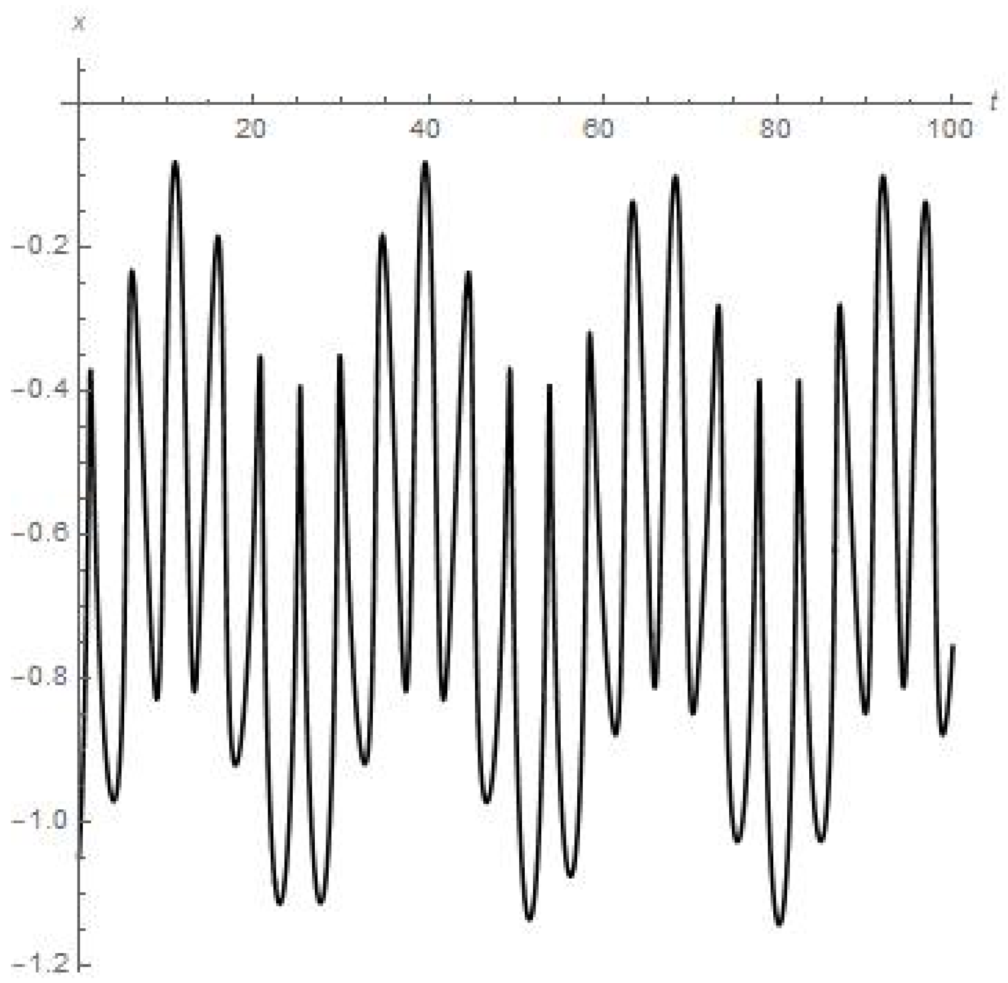
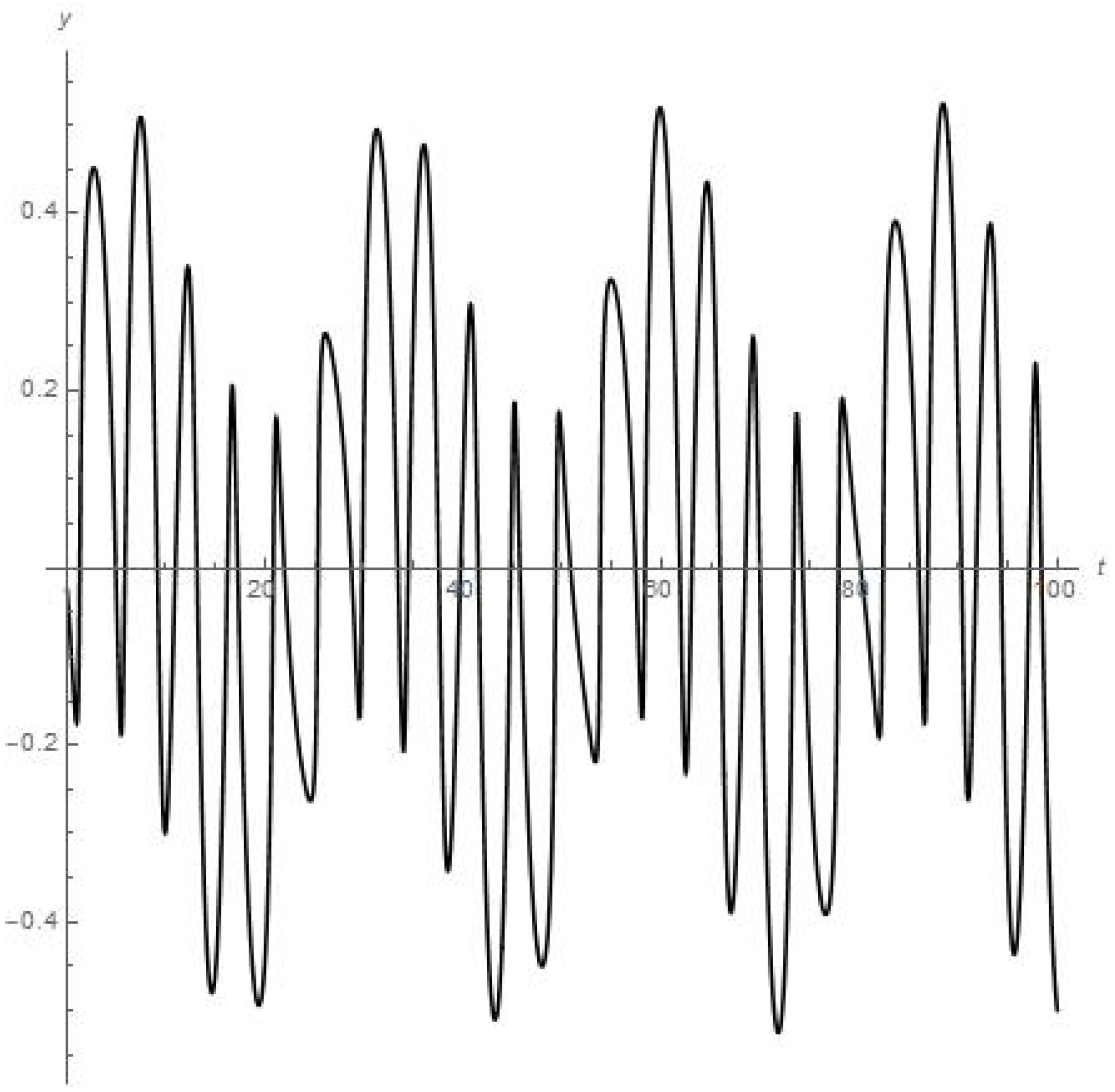
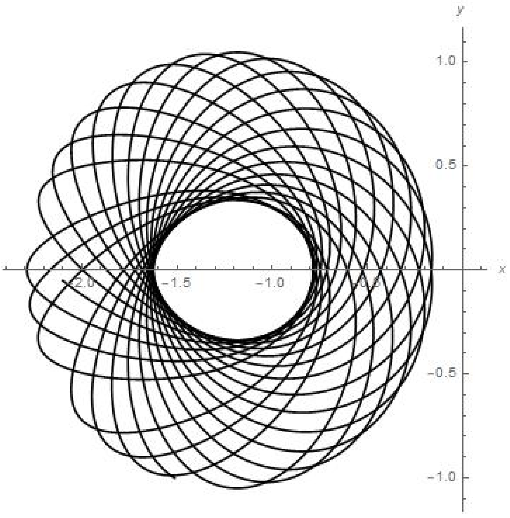
Figure 1 and Figure 2 present the results of numerical experiment for the coordinates {x, y}. We can see that coordinates {x, y} are oscillating, each in a stable regime over a long period of time t (e.g., coordinate y experiences eight peaks of oscillations over 28 days or the first full angular turn of the moon around Earth starting from the initial point);

–

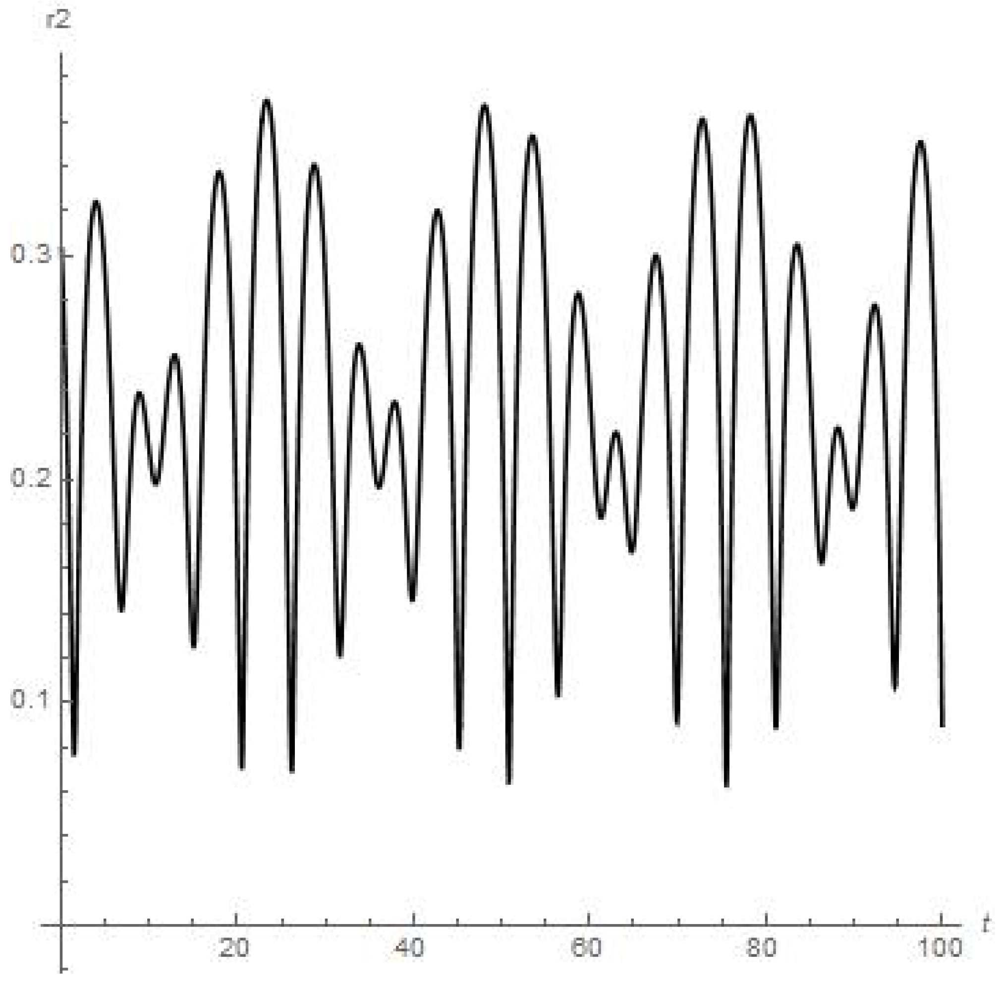
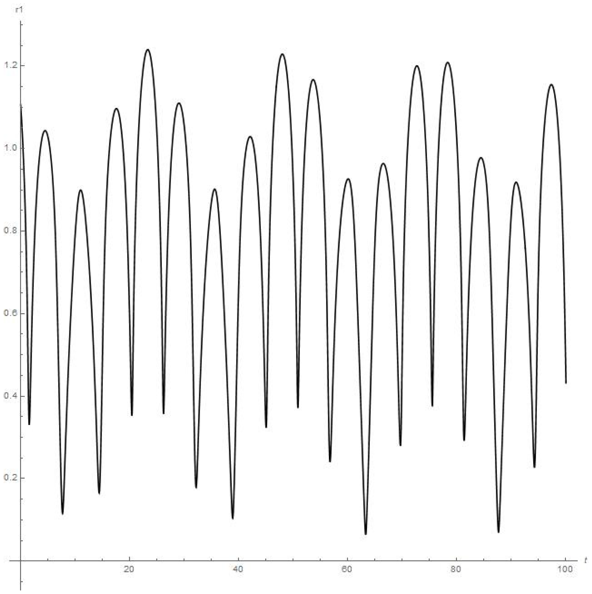
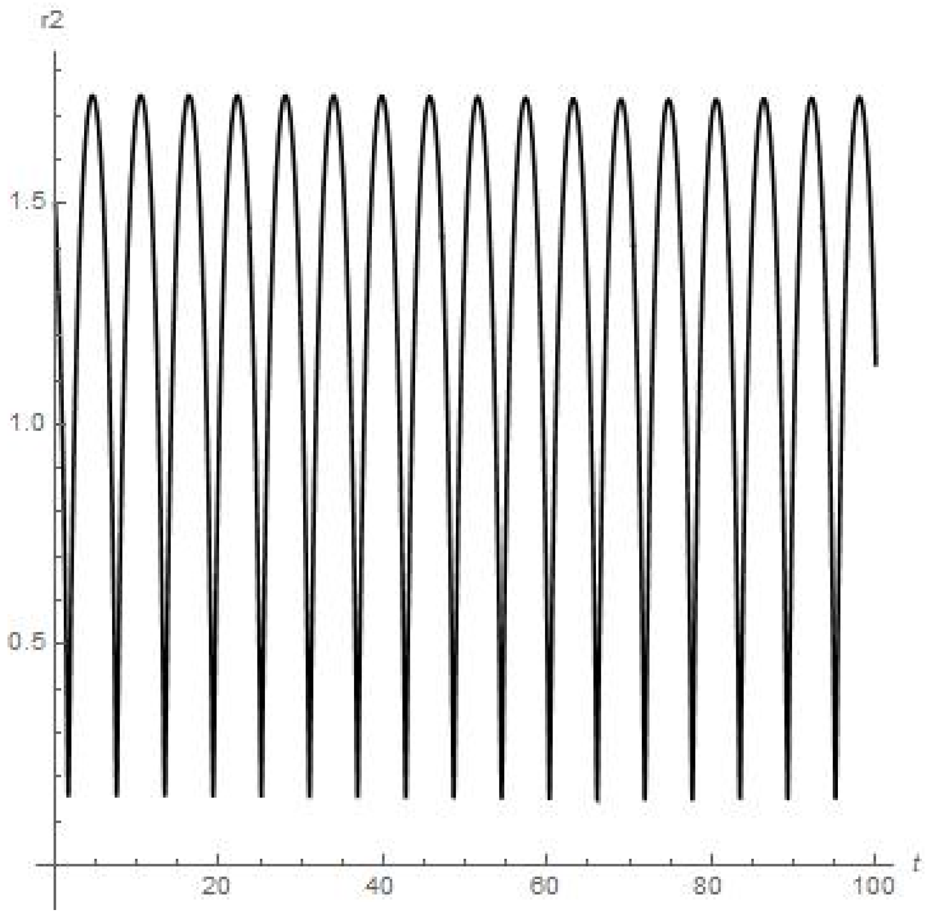
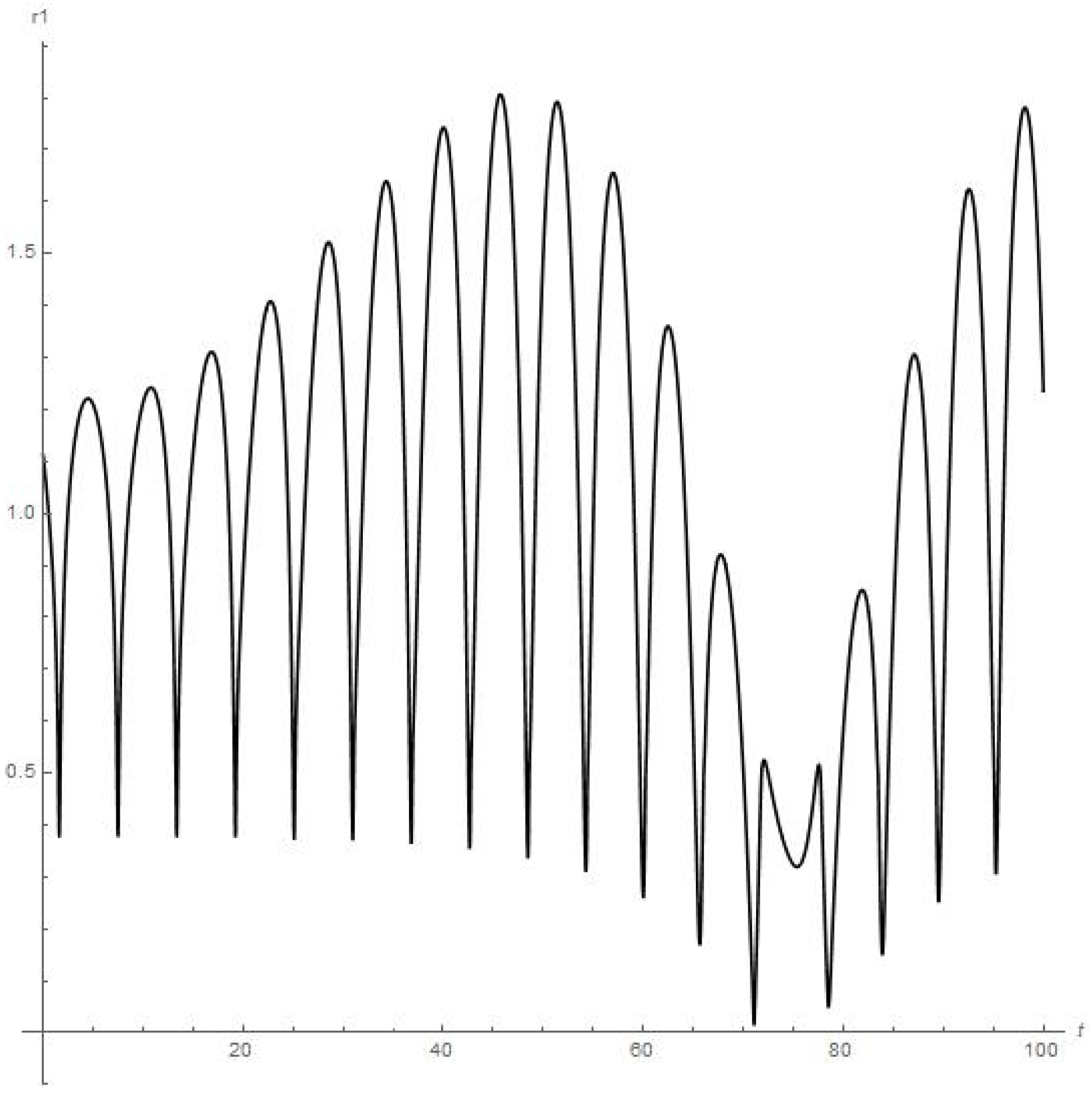
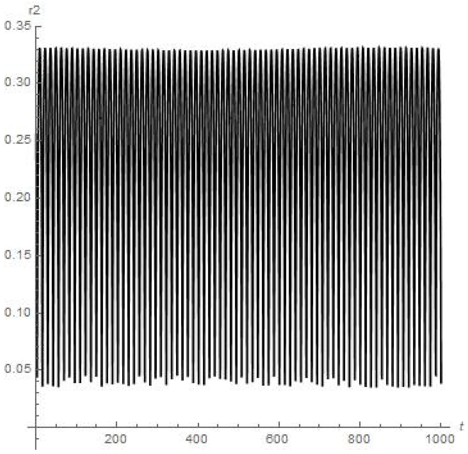
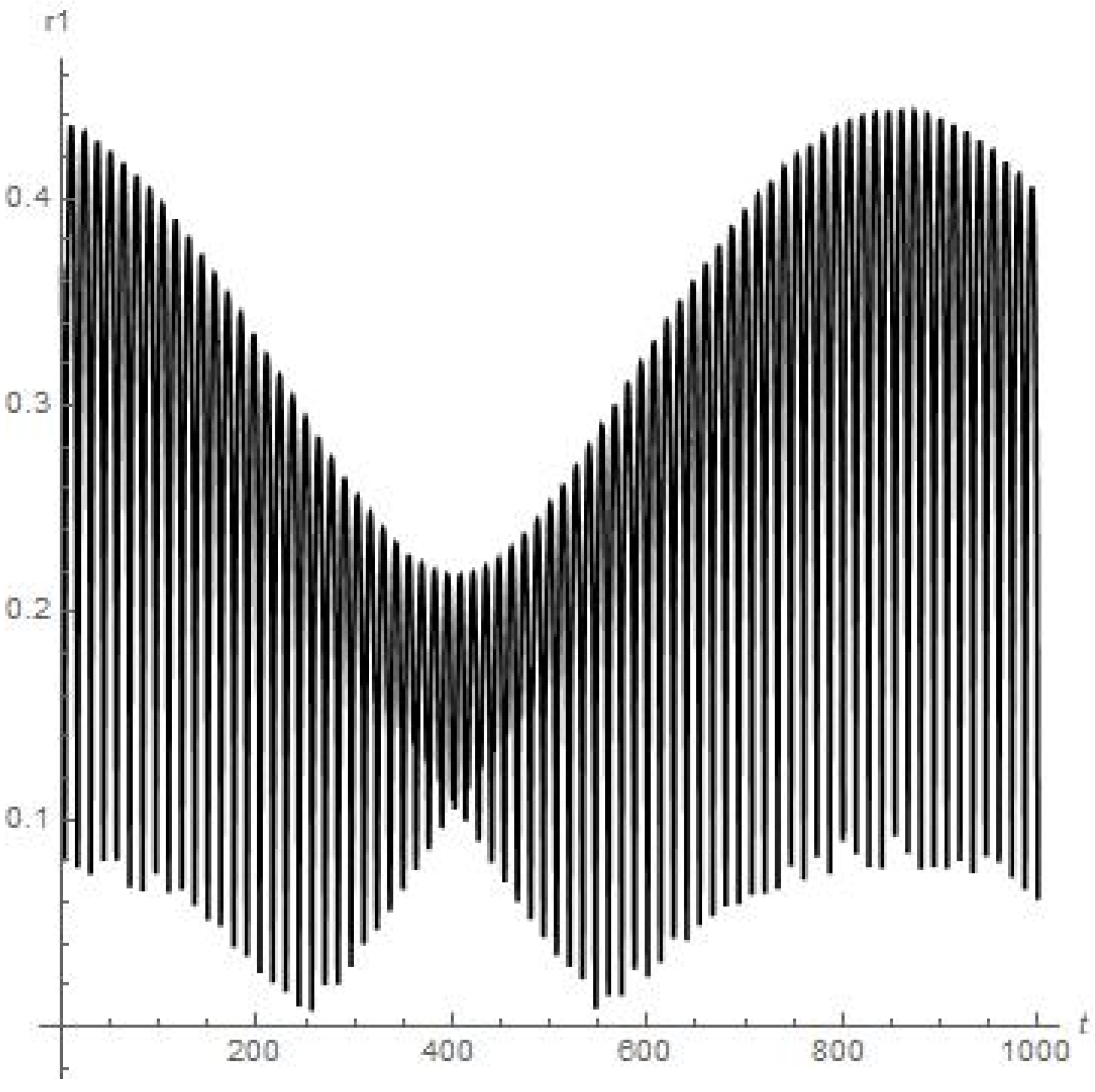
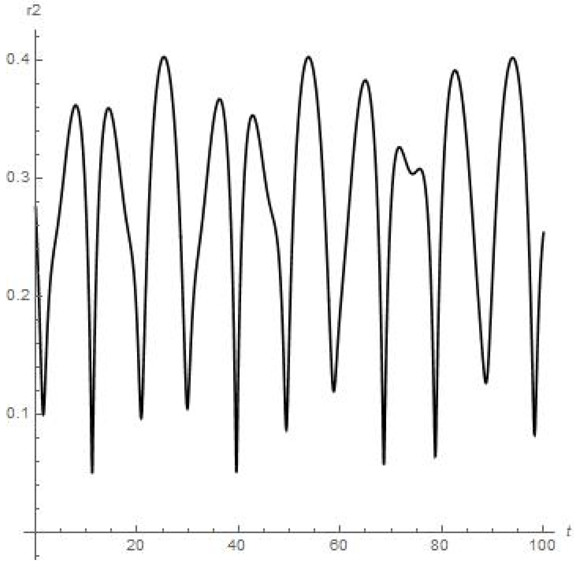
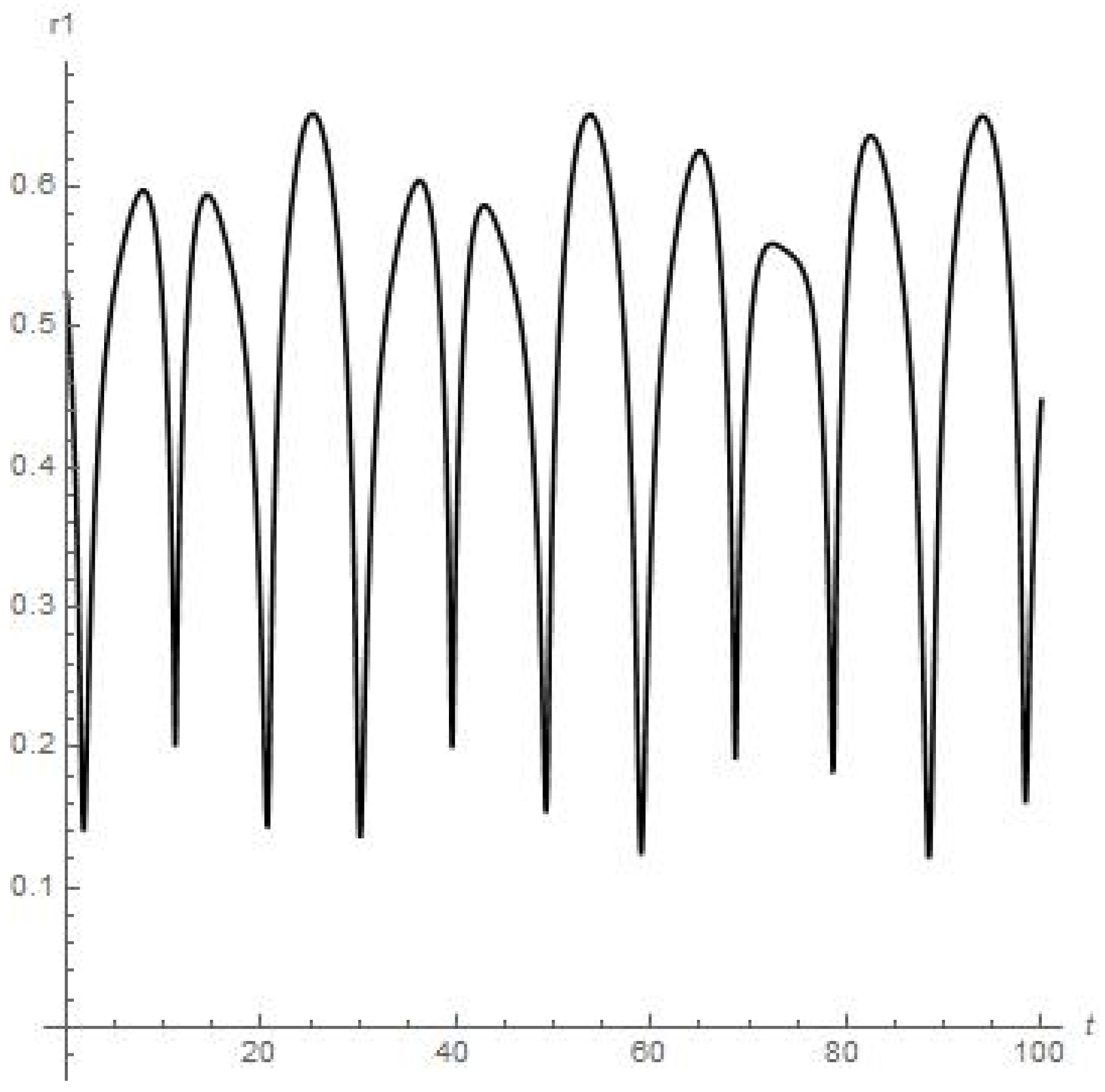
Figure 3 and Figure 4 present the results of the numerical calculations for the distances $r_{ 2}$, $r_{ 1}$ of planetoid m from the moon and from Earth, respectively. Namely, we can see from Figure 3 that distance $r_{ 2}$ is stably oscillating (there are also six peaks of oscillations over 28 days or the first full angular turn of the moon around Earth starting from the initial point) with an obvious further approx. stable regime over a long period of time. But the orbiter experiences a sufficiently close approach to Earth at the 63th day of orbiting around the moon (0.06 on Figure 4 or circa 23 × ${10}^3$ km);

–

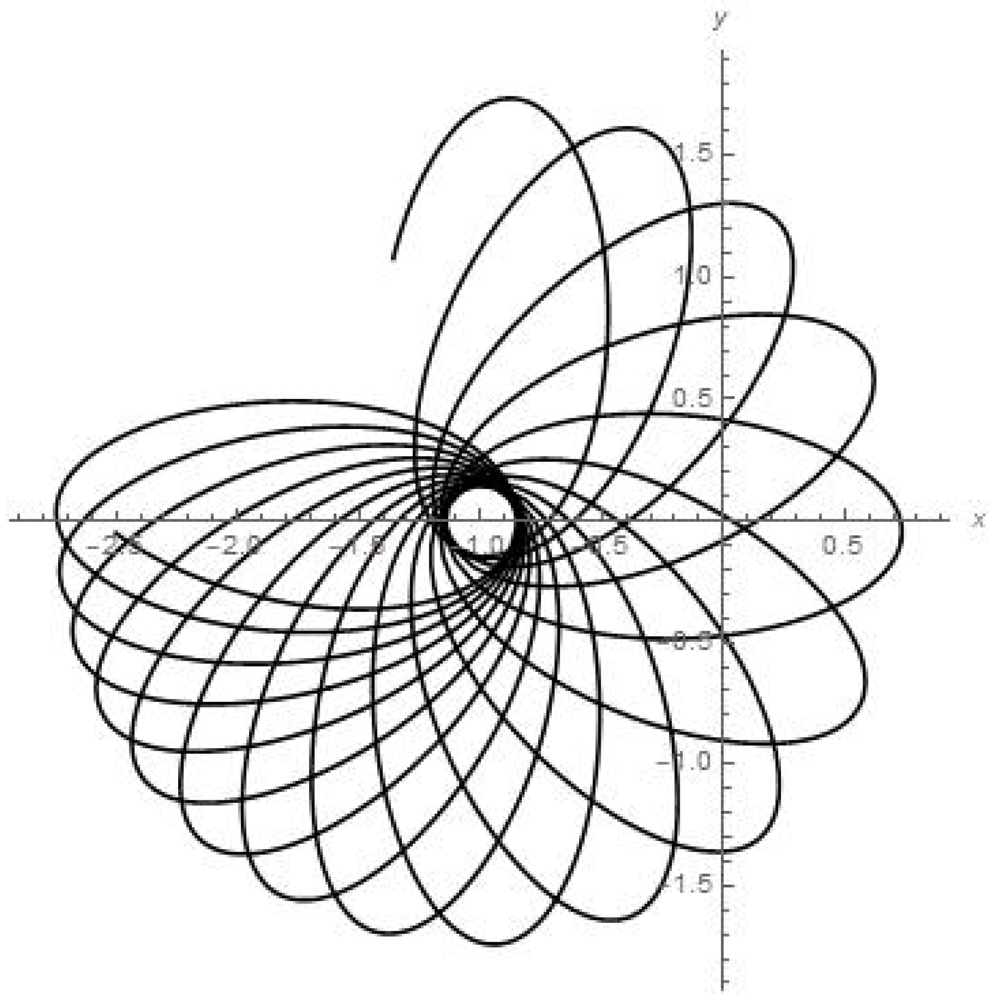
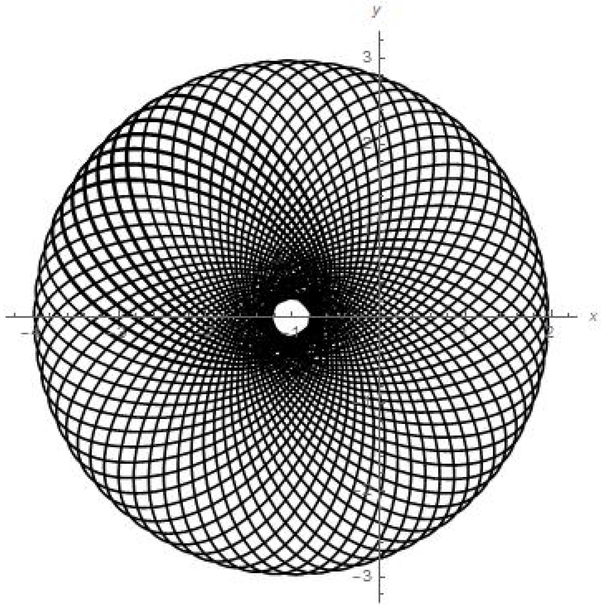
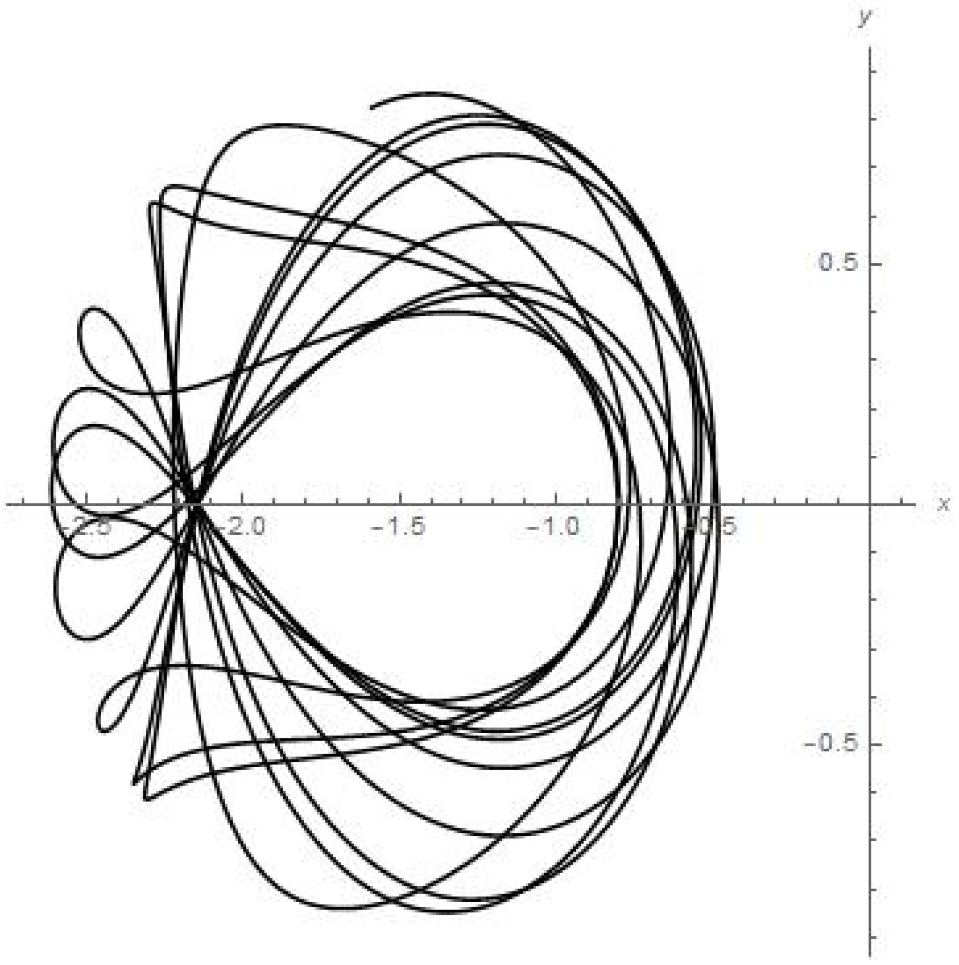
Figure 5 presents the numerical calculations for the trajectory of the planetoid in {x, y} plane. We can see that the small satellite is apparently stably oscillating with a shifted rate of angle precession around its initial position (of beginning the motion) in its quasi-elliptic trajectory between the attracting mass of Earth and attracting mass of the moon.

Last but not least, we should report our results for the cases of the moons of Mars (Phobos in Figure 6, Figure 7 and Figure 8 and Deimos in Figure 9, Figure 10 and Figure 11) and one of four large satellites of Jupiter, Callisto in Figure 12, Figure 13 and Figure 14 (there are four large satellites of Jupiter: Ganymede, Callisto, Io and Europa, but three of them—Ganymede, Io and Europa—are known to be captured in the Laplace resonance [16] and cannot be considered for the aims of our research). As we can see, there are no stable dynamics for satellites of moons for all these cases, except in the trio of “Jupiter-Callisto-planetoid”.

As we can see from Figure 6, Figure 7, Figure 8, Figure 9, Figure 10 and Figure 11, the dynamics of the finite-sized satellite near each of the moons of Mars is stable (but orbiter experiences a very close encounter with the surface of Mars at the 71st day of orbiting around Phobos). While the numerical calculations for the dynamics of the finite-sized planetoid m in the case of Jupiter (Figure 14) demonstrate to us that this small celestial body experiences stable orbiting, having at least two points in its trajectory where a strong change in regime “acceleration/deceleration” should disrupt such a small satellite in a mechanical way, due to it much exceeding the body tensile strength when moving near the Callisto in the “Jupiter-Callisto-satellite” system (the maximal close approach of the planetoid to Callisto in the {x, y, 0} plane is circa 0.055).

6. Discussion and Conclusions

In the current study, we explore the stability of motion of a finite-sized satellite around the natural moons of planets in the solar system using the novel concept of ER3BP with variable eccentricity. This concept was introduced earlier when a novel type of ER3BP (sun-planet-satellite) was investigated with a variable spin state of a secondary planet correlated implicitly to the motion of a satellite in the synodic co-rotating Cartesian coordinate system for its trapped orbit near the secondary planet (which is involved in the Kepler duet “Sun-planet”). But it is of real interest to explore another kind of problem described previously, plane ER3BP (planet-moon-satellite) with respect to the investigation of the motion of a finite-sized satellite m around the natural moon m_moon of a planet in the solar system with variable eccentricity of the moon in its motion in a fixed plane (invariable plane) around the planet. So, we considered here two primaries, M_planet and m_moon; the latter is orbiting around their common barycenter in a quasi-elliptic orbit with slow-changing eccentricity (on a large time scale) due to tidal phenomena. Our aim was to investigate the motion of a small finite-sized satellite around the natural moon of a planet in a quasi-stable elliptic orbit. Both novel theoretical and numerical findings (for various cases of trio “planet-moon-satellite”) are presented in the current research.

We should note that the results presented here, by approximated Equations (12) or (14) (see Figure 1, Figure 2, Figure 3, Figure 4, Figure 5, Figure 6, Figure 7, Figure 8, Figure 9, Figure 10, Figure 11, Figure 12, Figure 13 and Figure 14), could also be achieved by considering the more general case of the satellite’s form with respect to the simplified case k = 2h in (2). In addition, it is worth noting that the distance of the small mass m (satellite) from the moon should exceed the level of minimal distances not less than double Roche limit for this celestial body [9].

Also, the remarkable additional articles should be cited, which concern the problem under consideration, such as those of references [18,19,20,21,22,23,24,25,26,27,28,29,30,31,32,33,34,35,36,37,38,39,40,41,42,43,44,45,46,47,48,49,50,51,52,53,54,55,56,57,58,59,60,61,62,63,64,65,66,67]. To finalize our conclusions, let us remark that there is an old competitive discussion between members of the celestial mechanics community regarding which concept should be used:

(1)

constant Q for tidal evolution (not our choice; for example, see reference [34]);

(2)

approximation assuming “constant time lag” in the equilibrium tide model of tidal friction (this model was used, e.g., in the REBOUND integrator, see reference [35]);

(3)

the quality factor Q of the primary is assumed to be dependent on the tidal-flexure frequency (definitely our choice; see reference [17]).

Furthermore, modern approaches to orbital motions with tides (e.g., see the REBOUND integrator [35]) use numerical schemes that evaluate all the perturbations/forces at each timestep and can evolve a “Planet-moon-satellite” system for millions of years (~${10}^{ 9}$ submoon orbits). Moreover, these numerical approaches also consider the tides raised on the host bodies (e.g., planet and moon) by the host star that alter the exchange of angular momentum between the bodies. The current work includes these extra forces for possible consideration in the case of “Jupiter-Callisto-satellite” (since Jupiter should be considered as a “fluid-type planet” with another type of expression (8) presenting the dependence of low eccentricity e on true anomaly f and the dependence of true anomaly f on time t).

So, in this research we present the actual and novel algorithm for calculating the orbit of a finite-sized submoon in the conception of ER3BP for the “Planet-moon-satellite” trio (with slowly changing low eccentricity of the moon), both for a “rigid-type planet”, such as Earth or Mars (11), and the “fluid-type planet” Jupiter (8), confirming the utility/accuracy of the derived expressions for such an orbit.

References

1. Cabral, F.; Gil, P. On the Stability of Quasi-Satellite Orbits in the Elliptic Restricted Three-Body Problem. Master’s Thesis, Universidade Técnica de Lisboa, Lisbon, Portugal, 2011. [Google Scholar]
2. Arnold, V. Mathematical Methods of Classical Mechanics; Springer: New York, NY, USA, 1978. [Google Scholar]
3. Duboshin, G.N. Nebesnaja Mehanika. Osnovnye Zadachi i Metody. In Handbook for Celestial Mechanics; Nauka: Moscow, Russia, 1968. (In Russian) [Google Scholar]
4. Szebehely, V. Theory of Orbits. In The Restricted Problem of Three Bodies; Yale University: New Haven, Connecticut; Academic Press: New York, NY, USA; London, UK, 1967. [Google Scholar]
5. Abouelmagd, E.I.; Pal, A.K.; Guirao, J.L. Analysis of nominal halo orbits in the Sun–Earth system. Arch. Appl. Mech. 2021, 91, 4751–4763. [Google Scholar] [CrossRef]
6. Ferrari, F.; Lavagna, M. Periodic motion around libration points in the Elliptic Restricted Three-Body Problem. Nonlinear Dyn. 2018, 93, 453–462. [Google Scholar] [CrossRef]
7. Llibre, J.; Conxita, P. On the elliptic restricted three-body problem. Celest. Mech. Dyn. Astron. 1990, 48, 319–345. [Google Scholar] [CrossRef]
8. Ershkov, S.; Aboeulmagd, E.; Rachinskaya, A. A novel type of ER3BP introduced for hierarchical configuration with variable angular momentum of secondary planet. Arch. Appl. Mech. 2021, 91, 4599–4607. [Google Scholar] [CrossRef]
9. Ershkov, S.; Rachinskaya, A. Semi-analytical solution for the trapped orbits of satellite near the planet in ER3BP. Arch. Appl. Mech. 2021, 91, 1407–1422. [Google Scholar] [CrossRef]
10. Ershkov, S.; Leshchenko, D.; Rachinskaya, A. Note on the trapped motion in ER3BP at the vicinity of barycenter. Arch. Appl. Mech. 2021, 91, 997–1005. [Google Scholar] [CrossRef]
11. Ashenberg, J. Satellite pitch dynamics in the elliptic problem of three bodies. J. Guid. Control Dyn. 1996, 1, 68–74. [Google Scholar] [CrossRef]
12. Ershkov, S.; Leshchenko, D.; Rachinskaya, A. Revisiting the dynamics of finite-sized satellite near the planet in ER3BP. Arch. Appl. Mech. 2022, 92, 2397–2407. [Google Scholar] [CrossRef]
13. Ershkov, S.; Leshchenko, D.; Rachinskaya, A. Capture in regime of a trapped motion with further inelastic collision for finite-sized asteroid in ER3BP. Symmetry 2022, 14, 1548. [Google Scholar] [CrossRef]
14. Abouelmagd, E.I.; Ansari, A.A.; Ullah, M.S.; García Guirao, J.L. A Planar Five-body Problem in a Framework of Heterogeneous and Mass Variation Effects. Astron. J. 2020, 160, 216. [Google Scholar] [CrossRef]
15. Ershkov, S.; Leshchenko, D.; Aboeulmagd, E. About influence of differential rotation in convection zone of gaseous or fluid giant planet (Uranus) onto the parameters of orbits of satellites. Eur. Phys. J. Plus 2021, 136, 387. [Google Scholar] [CrossRef]
16. Ershkov, S.; Leshchenko, D. On the stability of Laplace resonance for Galilean moons (Io, Europa, Ganymede). An. Acad. Bras. Ciências Ann. Braz. Acad. Sci. 2021, 93, e20201016. [Google Scholar] [CrossRef]
17. Ershkov, S.V. About tidal evolution of quasi-periodic orbits of satellites. Earth Moon Planets 2017, 1201, 15–30. [Google Scholar] [CrossRef] [Green Version]
18. Ershkov, S.V.; Leshchenko, D. Solving procedure for 3D motions near libration points in CR3BP. Astrophys. Space Sci. 2019, 364, 207. [Google Scholar] [CrossRef] [Green Version]
19. Ershkov, S.; Leshchenko, D.; Prosviryakov, E.Y. A novel type of ER3BP introducing Milankovitch cycles or seasonal irradiation processes influencing onto orbit of planet. Arch. Appl. Mech. 2023, 93, 813–822. [Google Scholar] [CrossRef]
20. Singh, J.; Umar, A. On motion around the collinear libration points in the elliptic R3BP with a bigger triaxial primary. New Astron. 2014, 29, 36–41. [Google Scholar] [CrossRef]
21. Lukyanov, L.G.; Uralskaya, V.S. Sundman Stability of Natural Planet Satellites. Mon. Not. R. Astron. Soc. 2012, 421, 2316–2324. [Google Scholar] [CrossRef] [Green Version]
22. Lukyanov, L.G.; Uralskaya, V.S. Hill stability of natural planet satellites in the restricted elliptic three-body problem. Sol. Syst. Res. 2015, 49, 263–270. [Google Scholar] [CrossRef]
23. Ciccarelli, E.; Baresi, N. Covariance Analysis of Periodic and Quasi-Periodic Orbits around Phobos with Applications to the Martian Moons Exploration Mission. Astrodynamics 2023, in press. [Google Scholar] [CrossRef]
24. Nekhoroshev, N.N. Exponential estimate on the stability time of near integrable Hamiltonian systems. Russ. Math. Surv. 1977, 32, 5–66. (In Russian) [Google Scholar] [CrossRef]
25. Lidov, M.L.; Vashkov’yak, M.A. Theory of perturbations and analysis of the evolution of quasi-satellite orbits in the restricted three-body problem. Kosm. Issled. 1993, 31, 75–99. [Google Scholar]
26. Peale, S.J. Orbital Resonances In The Solar System. Annu. Rev. Astron. Astro-Phys. 1976, 14, 215–246. [Google Scholar] [CrossRef]
27. Wiegert, P.; Innanen, K.; Mikkola, S. The stability of quasi satellites in the outer solar system. Astron. J. 2000, 119, 1978–1984. [Google Scholar] [CrossRef] [Green Version]
28. Lhotka, C. Nekhoroshev Stability in the Elliptic Restricted Three Body Problem. Ph.D. Thesis, Wien University, Wien, Austria, 2008. [Google Scholar] [CrossRef]
29. Singh, J.; Leke, O. Stability of the photogravitational restricted three-body problem with variable masses. Astrophys. Space Sci. 2010, 326, 305–314. [Google Scholar] [CrossRef]
30. Shankaran, S.; Sharma, J.P.; Ishwar, B. Equilibrium points in the generalized photogravitational non-planar restricted three body problem. Int. J. Eng. Sci. Technol. 2011, 3, 63–67. [Google Scholar] [CrossRef]
31. Alshaery, A.A.; Abouelmagd, E.I. Analysis of the spatial quantized three-body problem. Results Phys. 2020, 17, 103067. [Google Scholar] [CrossRef]
32. Chernikov, Y.A. The Photogravitational Restricted Three-Body Problem. Sov. Astron. 1970, 14, 176. [Google Scholar]
33. Gomes, V.M.; de Cássia Domingos, R. Studying the lifetime of orbits around Moons in elliptic motion. Comp. Appl. Math. 2016, 35, 653–661. [Google Scholar] [CrossRef]
34. Emelyanov, N.V. Influence of tides in viscoelastic bodies of planet and satellite on the satellite’s orbital motion. Mon. Not. R. Astron. Soc. 2018, 479, 1278–1286. [Google Scholar] [CrossRef]
35. Lu, T.; Rein, H.; Tamayo, D.; Hadden, S.; Mardling, R.; Millholland, S.C.; Laughlin, G. Self-consistent Spin, Tidal, and Dynamical Equations of Motion in the REBOUNDx Framework. Astrophys. J. 2023, 948, 41. [Google Scholar] [CrossRef]
36. Ferraz-Mello, S.; Rodríguez, A.; Hussmann, H. Tidal friction in close-in satellites and exoplanets: The Darwin theory re-visited. Celest. Mech. Dyn. Astron. 2008, 101, 171–201. [Google Scholar] [CrossRef] [Green Version]
37. Sidorenko, V.V. The eccentric Kozai–Lidov effect as a resonance phenomenon. Celest. Mech. Dyn. Astron. 2018, 130, 4. [Google Scholar] [CrossRef] [Green Version]
38. Efroimsky, M.; Lainey, V. Physics of bodily tides in terrestrial planets and the appropriate scales of dynamical evolution. J. Geophys. Res. 2007, 112, E12003. [Google Scholar] [CrossRef]
39. Efroimsky, M.; Makarov, V.V. Tidal friction and tidal lagging. Applicability limitations of a popular formula for the tidal torque. Astrophys. J. 2013, 764, 10. [Google Scholar] [CrossRef] [Green Version]
40. Peale, S.J.; Cassen, P. Contribution of Tidal Dissipation to Lunar Thermal History. Icarus 1978, 36, 245–269. [Google Scholar] [CrossRef]
41. Ershkov, S.; Leshchenko, D.; Prosviryakov, E. Revisiting Long-Time Dynamics of Earth’s Angular Rotation Depending on Quasiperiodic Solar Activity. Mathematics 2023, 11, 2117. [Google Scholar] [CrossRef]
42. Mel’nikov, A.V.; Orlov, V.V.; Shevchenko, I.I. The Lyapunov exponents in the dynamics of triple star systems. Astron. Rep. 2013, 57, 429–439. [Google Scholar] [CrossRef]
43. Mel’nikov, A.V.; Shevchenko, I.I. Unusual rotation modes of minor planetary satellites. Sol. Syst. Res. 2007, 41, 483–491. [Google Scholar] [CrossRef]
44. Shalini, K.; Idrisi, M.J.; Singh, J.K.; Ullah, M.S. Stability analysis in the R3BP under the effect of heterogeneous spheroid. New Astron. 2023, 104, 102056. [Google Scholar] [CrossRef]
45. Lidov, M.L. Evolution of the orbits of artificial satellites of planets as affected by gravitational perturbation from external bodies. AIAA J. 1963, 1, 1985–2002. [Google Scholar] [CrossRef]
46. de Almeida Prado, A.F.B. Third-Body Perturbation in Orbits Around Natural Satellites. J. Guid. Control Dyn. 2003, 26, 33–40. [Google Scholar] [CrossRef]
47. Ershkov, S.; Leshchenko, D.; Prosviryakov, E.Y. Semi-Analytical Approach in BiER4BP for Exploring the Stable Positioning of the Elements of a Dyson Sphere. Symmetry 2023, 15, 326. [Google Scholar] [CrossRef]
48. Ansari, A.A.; Prasad, S.N. Generalized elliptic restricted four-body problem with variable mass. Astron. Lett. 2020, 46, 275–288. [Google Scholar] [CrossRef]
49. Ershkov, S.V. The Yarkovsky effect in generalized photogravitational 3-body problem. Planet. Space Sci. 2012, 73, 221–223. [Google Scholar] [CrossRef] [Green Version]
50. Liu, C.; Gong, S. Hill stability of the satellite in the elliptic restricted four-body problem. Astrophys. Space Sci. 2018, 363, 162. [Google Scholar] [CrossRef]
51. Meena, P.; Kishor, R. First order stability test of equilibrium points in the planar elliptic restricted four body problem with radiating primaries. Chaos Solitons Fractals 2021, 150, 111138. [Google Scholar] [CrossRef]
52. Umar, A.; Jagadish, S. Semi-analytic solutions for the triangular points of double white dwarfs in the ER3BP: Impact of the body’s oblateness and the orbital eccentricity. Adv. Space Res. 2015, 55, 2584–2591. [Google Scholar] [CrossRef]
53. Idrisi, M.J.; Ullah, M.S. A Study of Albedo Effects on Libration Points in the Elliptic Restricted Three-Body Problem. J. Astronaut. Sci. 2020, 67, 863–879. [Google Scholar] [CrossRef]
54. Younis, S.H.; Ismail, M.N.; Mohamdien, G.F.; Ibrahiem, A.H. Effects of Radiation Pressure on the Elliptic Restricted Four-Body Problem. J. Appl. Math. 2021, 2021, 5842193. [Google Scholar] [CrossRef]
55. Vincent, A.E.; Perdiou, A.E.; Perdios, E.A. Existence and Stability of Equilibrium Points in the R3BP With Triaxial-Radiating Primaries and an Oblate Massless Body Under the Effect of the Circumbinary Disc. Front. Astron. Space Sci. 2022, 9, 877459. [Google Scholar] [CrossRef]
56. Cheng, H.; Gao, F. Periodic Orbits of the Restricted Three-Body Problem Based on the Mass Distribution of Saturn’s Regular Moons. Universe 2022, 8, 63. [Google Scholar] [CrossRef]
57. Umar, A.; Hussain, A. A Motion in the ER3BP with an oblate primary and a triaxial stellar companion. Astrophys. Space Sci. 2016, 361, 344. [Google Scholar] [CrossRef]
58. Singh, J.; Umar, A. Effect of Oblateness of an Artificial Satellite on the Orbits Around the Triangular Points of the Earth–Moon System in the Axisymmetric ER3BP. Differ. Equ. Dyn. Syst. 2017, 25, 11–27. [Google Scholar] [CrossRef]
59. Emel’yanov, N.V.; Kanter, A.A. Orbits of new outer planetary satellites based on observations. Sol. Syst. Res. 2005, 39, 112–123. [Google Scholar] [CrossRef]
60. Emel’yanov, N.V. Visible Encounters of the Outermost Satellites of Jupiter. Sol. Syst. Res. 2001, 35, 209–211. [Google Scholar] [CrossRef]
61. Emelyanov, N.V.; Vashkov’yak, M.A. Evolution of orbits and encounters of distant planetary satellites. Study tools and examples. Sol. Syst. Res. 2012, 46, 423–435. [Google Scholar] [CrossRef]
62. Emelyanov, N.V. Dynamics of Natural Satellites of Planets Based on Observations. Astron. Rep. 2018, 62, 977–985. [Google Scholar] [CrossRef]
63. Emelyanov, N.V.; Drozdov, A.E. Determination of the orbits of 62 moons of asteroids based on astrometric observations. Mon. Not. R. Astron. Soc. 2020, 494, 2410–2416. [Google Scholar] [CrossRef]
64. Emelyanov, N. The Dynamics of Natural Satellites of the Planets; Elsevier: Amsterdam, The Netherlands, 2021; 501p, ISBN 978-0-12-822704-6. [Google Scholar] [CrossRef]
65. Emelyanov, N.V.; Arlot, J.E.; Varfolomeev, M.I.; Vashkov’yak, S.N.; Kanter, A.A.; Kudryavtsev, S.M.; Nasonova, L.P.; Ural’skaya, V.S. Construction of theories of motion, ephemerides, and databases for natural satellites of planets. Cosm. Res. 2006, 44, 128–136. [Google Scholar] [CrossRef]
66. Abouelmagd, E.I.; García Guirao, J.L.; Pal, A.K. Periodic solution of the nonlinear Sitnikov restricted three-body problem. New Astron. 2020, 75, 101319. [Google Scholar] [CrossRef]
67. Luk’yanov, L.G.; Shirmin, G.I. On the Hill stability in the general problem of three finite bodies. Astron. Lett. 2002, 28, 419–422. [Google Scholar] [CrossRef]
Figure 1. Results of numerical calculations of the coordinate x.
Mathematics 11 03147 g001
Figure 2. Results of numerical calculations of the coordinate y.
Mathematics 11 03147 g002
Figure 3. Results of numerical calculations of the r 2 . Orbiter experiences close encounter with moon at 25th day of orbiting around Earth’s Moon.
Mathematics 11 03147 g003
Figure 4. Results of numerical calculations of the r 1 .
Mathematics 11 03147 g004
Figure 5. Results of numerical calculations for trajectory in {x, y} plane.
Mathematics 11 03147 g005
Figure 6. Results of numerical calculations of the r 2 for satellite of Phobos, moon of Mars (up to meaning t = 100). Initial conditions are chosen as previously in Figure 1 and Figure 2; µ ≅ (1.072 × 10 16 /6.42 × 10 24 ) ~ 0.167 × 10 8 , C = 6.2832/(7.66/24).
Mathematics 11 03147 g006
Figure 7. Results of numerical calculations of the r 1 for satellite of Phobos, moon of Mars (up to meaning t = 100). Orbiter experiences close encounter with upper atmosphere of Mars at 71st day of orbiting around Phobos.
Mathematics 11 03147 g007
Figure 8. Results of numerical calculations for trajectory in {x, y} plane for satellite of Phobos of Mars.
Mathematics 11 03147 g008
Figure 9. Results of numerical calculations of the r 2 for satellite of Deimos, moon of Mars (up to meaning t = 1000). Initial conditions are chosen as previously in Figure 1 and Figure 2; µ ≅ (1.48 × 10 15 /6.42 × 10 24 ) ~ 0.231 × 10 9 , C = 6.2832/(30.33/24).
Mathematics 11 03147 g009
Figure 10. Results of numerical calculations of the r 1 for satellite of Deimos, moon of Mars (up to meaning t = 1000). Orbiter experiences first close encounter with upper atmosphere of Mars at 250th day of orbiting around Deimos.
Mathematics 11 03147 g010
Figure 11. Results of numerical calculations for trajectory in {x, y} plane for satellite of Deimos of Mars.
Mathematics 11 03147 g011
Figure 12. Results of numerical calculations of the r 2 for satellite of Callisto, moon of Jupiter (up to meaning t = 100). Initial conditions are chosen as previously in Figure 1 and Figure 2; µ ≅ (1.075 × 10 23 /1.9 × 10 27 ) ~ 0.5658 × 10 4 , C = 6.2832/16.689.
Mathematics 11 03147 g012
Figure 13. Results of numerical calculations of the r 1 for satellite of Callisto, moon of Jupiter (up to meaning t = 100). Orbiter does not experience close encounter with upper atmosphere of Jupiter during process of orbiting around Callisto.
Mathematics 11 03147 g013
Figure 14. Results of numerical calculations for trajectory in {x, y} plane for satellite of Callisto, moon of Jupiter.
Mathematics 11 03147 g014
Disclaimer/Publisher’s Note: The statements, opinions and data contained in all publications are solely those of the individual author(s) and contributor(s) and not of MDPI and/or the editor(s). MDPI and/or the editor(s) disclaim responsibility for any injury to people or property resulting from any ideas, methods, instructions or products referred to in the content.