Article

Optimal Circular Economy and Process Maintenance Strategies for an Imperfect Production–Inventory Model with Scrap Returns

1
Department of Statistics and Information Science, Fu Jen Catholic University, New Taipei City 242062, Taiwan
2
Department of Marketing and Logistics Management, Chaoyang University of Technology, Taichung 413310, Taiwan
3
Department of Business Administration, Tamkang University, New Taipei City 251301, Taiwan
*
Authors to whom correspondence should be addressed.
Mathematics 2023, 11(14), 3041; https://doi.org/10.3390/math11143041
Submission received: 24 May 2023 / Revised: 20 June 2023 / Accepted: 5 July 2023 / Published: 8 July 2023
(This article belongs to the Special Issue Supply Chain Management and Mathematical Logistics)

Abstract

:
To protect our environment, current firms are committed to the circular economy and process maintenance strategies to reduce the waste of resources. In this way, they can also save costs and create an enterprise image and value. Therefore, this study explores an imperfect production system with a circular economy and process maintenance activities, wherein the defective products can be converted into scrap returns (i.e., secondary raw materials) and products can be manufactured using mixed materials containing scrap returns. The proposed system considers multiple products with varying feed rates of scrap returns. According to the scenario of the aforementioned production system, this paper develops a production–inventory model aimed at cost minimization, in which the production run time, purchased quantity of material, number of maintenance times, and recovery rate are decision variables. Furthermore, we also develop a computational algorithm to obtain these optimal solutions efficiently. Finally, the numerical and sensitivity analyses based on a practical case are presented to illustrate the applicability of our method and some managerial implications. For example, both strategies efficiently reduce the total cost per unit time in the proposed numerical example. The sensitivity results can be used to determine the optimal combination of two strategies and the execution moment under various changes in cost parameters.

1. Introduction

The economic production quantity (EPQ) model is common in research involving production–inventory problems. The primary objective of EPQ is to identify the optimal production quantity or production run time, with the aim of minimizing costs or maximizing profits. Drawing from the EPQ model’s structure, several researchers have incorporated diverse manufacturing scenarios into their models, enhancing their practicality in real-world applications. Multiple-stage production is a common system among them. For instance, products typically undergo arduous processing procedures, including molding, cutting, grinding, painting, assembling, and more. Inventory-related costs arise from the temporary storage of work-in-process goods between stations as a consequence of the varying production speeds at each processing station. Therefore, inventory management in a multi-stage production system is challenging from a practical and academic perspective.
The traditional linear economy pattern follows the take–make–dispose scheme [1], which leads to the irrational use of available resources. To protect our environment, current firms have committed to the circular economy for scrap recycling and low waste during the manufacturing process. According to the Ellen MacArthur Foundation [2], the most recent schematic diagram comparing the linear economy and the circular economy. highlights the recovery process taking place within the factory, which involves the conversion of defective products (or waste) into scrap returns. This process represents an inner circular economy and serves as a manifestation of green manufacturing, with the objective of reducing the usage of natural resources, pollution, and waste, promoting recycling and material reuse, and regulating emissions in various processes. Nowadays, numerous green manufacturing industries have adopted circular economy measures and achieved significant outcomes. One notable example is the utilization of sulfuric acid as a crucial raw material in the semiconductor etching process. Over the past few years, semiconductor manufacturers have dedicated themselves to investing in waste sulfuric acid purification technology to reduce the reliance on natural sulfur mining. In the manufacturing sectors of metal and plastic products, defective items can be repurposed into secondary raw materials by utilizing the melting process. The scrap metal industry is growing in the Sunyani Municipality, and a similar trend is likely to be observed in other cities in Ghana as well [3]. Paletta et al. [4] proposed accelerating the circularity of plastic-based material systems for radical innovations in Italy. Considering the principles of the circular economy, it becomes imperative to address significant aspects of circular systems, including reuse, sharing, repair, refurbishment, remanufacturing, and recycling. By doing so, a closed-loop system can be created, thereby effectively reducing the utilization of resources and carbon emissions. Accordingly, current firms are constantly developing reusable materials and processing equipment such that defective items and scrap can be converted into scrap returns (i.e., secondary raw materials). Not only can this help control costs by reducing waste, but it also serves as one of the implements of the circular economy, thereby improving the financial performance of enterprises. On the other hand, process maintenance activity can also be part of green manufacturing. Process maintenance is a common activity in current firms. It can avoid more defective products caused by equipment degradation through regular or irregular maintenance such that material is not wasted.
Based on the above-mentioned strategies involving low waste, this study would develop a multiple-stage and imperfect production–inventory model incorporating scrap returns and a controllable defective rate. Furthermore, the finished products are manufactured using mixed materials that include scrap returns. To avoid a lack or an unlimited accumulation of scrap returns, we consider two products with different feed rates of scrap returns in this production system. The joint economic order quantity (EOQ) model and the EPQ model are established, wherein the production run time, purchase quantity of material, number of maintenance times, and recovery rate are decision variables. The rest of this paper is organized as follows. Section 2 focuses on the review of the related literature and compares the differences between this study and prior research to highlight the contributions of our study. In Section 3, the notation and assumptions employed in the entire paper are established. Section 4 presents the mathematical formulations and theoretical results. Section 5 provides the solution procedure for this inventory model. Section 6 presents a numerical example to illustrate a solution procedure, followed by a sensitivity analysis based on this example in Section 7, which provides managerial insights and references for decision making. Finally, Section 8 concludes this paper and offers directions for future research.

2. Literature Review

For the production system regarded as multiple-stage, most studies have considered it in their production–inventory models. For instance, a two-stage production inventory system, considering imperfect production processes, preventive maintenance, and inspection, was modeled by Darwish and Ben-Daya [5]. Pearn et al. [6] developed a multiple-stage EPQ with an investment in quality improvement. Then, Chang et al. [7] further considered the variable assembly rate in the manual process. Sarkar and Shewchuk [8] proposed a production system with advanced demand information and early order fulfillment. Paul et al. [9] developed a disruption recovery model in a three-stage production inventory system. Wang and Chan [10] discussed a robust production problem involving inventory inaccuracies and time delays. The innovative maintenance problem of complement replacement in a multiple-stage production system with imperfect processes was presented by Su et al. [1]. In a recent study conducted by Su et al. [11], the impact of corporate social responsibility (CSR) activities in a two-stage assembly production system was investigated. The authors also presented a conceptual framework that links the appropriate timing and extent of CSR execution to the outcomes of marketing strategies. Other similar multi-stage production systems are discussed by Tayyab et al. [12], Wang and Shi [13], and Cui et al. [14].
As far as we know, it is difficult to achieve a perfect process in the actual manufacturing environment. To enhance the practicality of the production–inventory model in the real world, many scholars have established various assumptions for the imperfect process, such as constant defective rates, random defective rates, random machine breakdowns, and random state shifts (i.e., in-control stage to out-of-control stage). Chang et al. [7] considered a two-stage assembly system (automatic stage and manual stage) with constant defective rates. Pearn et al. [6] explored a two-stage imperfect production system with completely backlogged and constant defective rates. Paul et al. [9] proposed a recovery strategy for maintaining disruptions with random defective rates in a mixed production system. Sarkar and Shewchuk [8] proposed a new approach for production replenishment and order fulfillment in a mixed production system with random defective rates. Öztürk [15] considered a random machine breakdown in an imperfect production system. In addition, Öztürk [16] examined an imperfect production inventory system that involved rework, random breakdowns, and inspection costs. To perform an error-free inspection, Dey et al. [17] examined the effect of random defective rates (that obey a certain distribution) in an imperfect production system with random shifts. Dey et al. [18] developed a sustainable imperfect system with random shifts and selling-price demand. Huang et al. [19] proposed a coordination supply chain model in which the supplier’s system had random shifts and price-sensitive demand. Manna et al. [20] addressed important claims regarding the effect of carbon emission on an imperfect system with random shifts and no advance payment base. For the disposal of defective products, in addition to discarding or selling at a discount, most scholars have assumed that the defective products can be completely or partially reworked. In the real world, there exists another disposal method capable of creating value for defective products, known as scrap returns. Su et al. [21] proposed an imperfect system where defective products are transformed into scrap returns. However, the issue of scrap returns is rarely discussed in the literature involving multi-stage production–inventory systems. For convenience, Table 1 presents a brief comparison of the above-mentioned literature by types of stages, imperfect process, and disposal. From Table 1, it is easy to see that there is a research gap involving an imperfect production–inventory model with multiple stages, scrap returns, and maintenance. Therefore, we take this research gap as our research direction.

3. Notation and Assumptions

To facilitate the explanation of the research questions and the model establishment of this paper, the notation and assumptions used throughout this study are summarized as follows.

3.1. Notation

In order to develop the model, we present the following notation, which includes parameters and decision variables.

3.2. Assumptions

  • Consider a production line that is not perfect and that produces multiple products, with the availability of process maintenance. For simplicity, we first establish a production–inventory model with two products. The production cost and materials used for the two products are the same, and the materials used are a mixture of new materials and scrap returns. Figure 1 illustrates a schematic process of the production line.
  • The defective products can be processed to scrap returns after passing the conversion stage. The conversion stage is used to process defective products into usable secondary raw materials through some special equipment, such as a furnace, blender, and extractor. However, a portion of defective products cannot be processed to scrap returns due to the imperfect conversion process. This study considers that capital investment in recovery capacity improvement is available, assuming it increases with the recovery rate.
  • The process is not always in the in-control stage due to degraded equipment; it randomly shifts from the in-control stage to the out-of-control stage after a while, t 1 . In this study, t 1 is assumed to be a random variable with a normal distribution. That is, t 1 ~ N ( μ ,   σ ) , where μ and σ are the mean and standard deviation, respectively (please refer to Su et al. [12]).
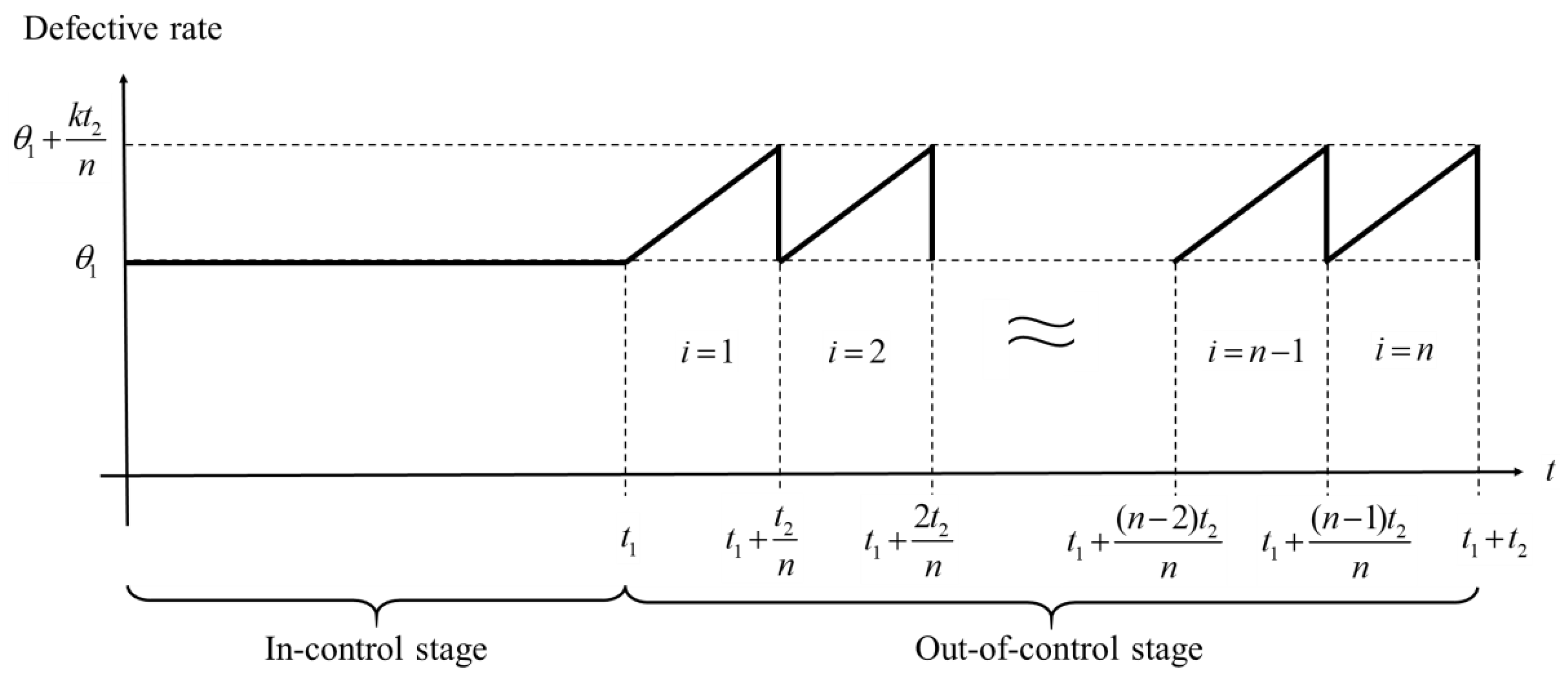
  • The defective rate during the in-control stage is constant and lower than or equal to that during the out-of-control stage, i.e., θ 1 θ 2 < 1 . In contrast, the defective rate during the out-of-control stage increases over time, but it can be returned to θ 1 after process maintenance. Note that process maintenance needs to be performed once for the next cycle after the end of the production system. However, if the maintenance cost is affordable, increasing the number of maintenance times during the out-of-control stage can reduce the waste of resources and indirectly increase production run time to retard the growth of the production cost. At this time, the number of maintenance times during the production cycle will be greater than one. Consequently, we will establish a generalized model for finding the optimal number of maintenance times. In this study, the defective rate during the out-of-control stage is set as the following linear function of time (denoted by g ( t ) ):
    θ 2 = g ( t ) = θ 1 + k t t 1 + ( i 1 ) t 2 n < 1 ,
    where t 1 + ( i 1 ) t 2 / n < t t 1 + i t 2 / n , i = 1 ,   2 ,   . . . . ,   n and k > 0 . Note that the maximum defective rate is θ 1 + k t 2 / n . Because the defective rate must be less than 1, there is a condition for a combination of decision variables, i.e., t 2 / n < ( 1 θ 1 ) / k . Figure 2 shows the change in the defective rate over time during a cycle.
  • It is assumed that the feed rates of scrap returns for two products are different and that they satisfy the inequality, f r ,   1 < f r ,   2 . Generally, product 1 and product 2 are arranged for manufacture in the in-control and out-of-control stages, respectively. In the in-control stage, the feed rate of scrap returns must be less than the recovery rate to avoid a lack of scrap returns, i.e., f r , 1   <   p f θ 1 r . On the contrary, the feed rate of scrap returns should exceed the recovery rate to avoid an unrestricted accumulation of scrap returns in the out-of-control stage, i.e., f r , 2   >   p f θ 2 r . Consequently, the inequality, f r , 1   <   p f θ 1 r     p f θ 2 r < f r ,   2 , is held, which implies the recovery rate, r ( f r , 1 / p f θ 1 ,   f r ,   2 / p f θ 2 ) .
  • To avoid shortages in sales, the production rate of the finished product is assumed to exceed the demand rate, i.e., p f ( 1 θ 1 ) > d 1 and p f ( 1 θ 2 ) > d 2 .

4. Model Formulation

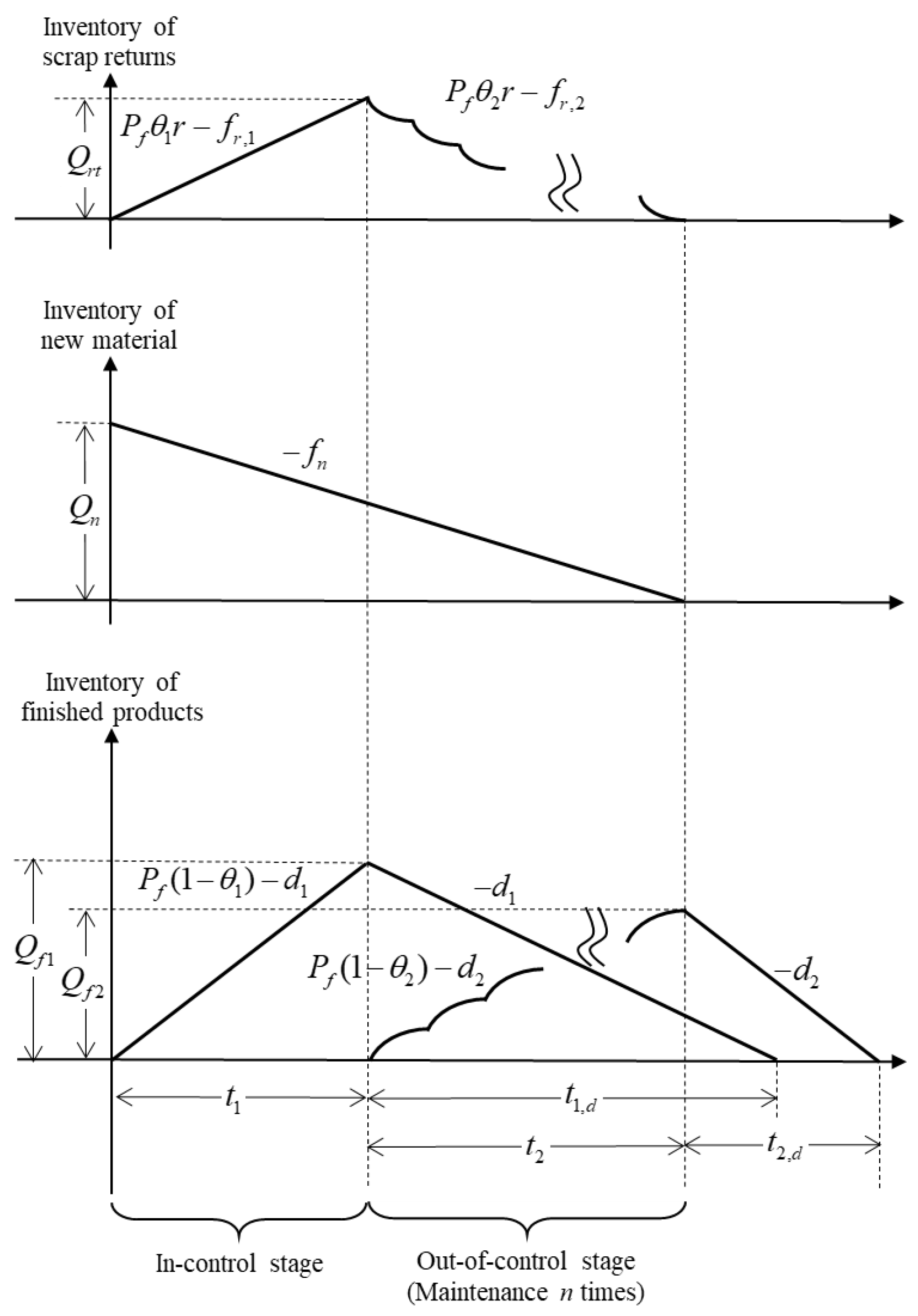
Based on the notation and assumptions listed in the previous section, an EPQ model describing the imperfect production–inventory system with recovery and maintenance activities can be established. The main objective is to find the optimal production run time, the number of maintenance times, the purchasing quantity of new material per cycle, and the recovery rate, while minimizing the total cost per unit time. First, Figure 3 presents the inventory levels of scrap returns, new material, and finished products throughout a cycle. As for the inventory level of scrap returns, it increases during the in-control stage (i.e., p f θ 1 r f r , 1 > 0 ) while it decreases during the out-of-control stage (i.e., p f θ 2 r f r , 2 < 0 ) based on Assumption (4). For the inventory level of new materials, the amount of Q n is purchased from the supplier at the beginning of the cycle, and then it gradually depletes to zero over time with the rate f n < 0 . For the inventory level of finished products, according to Assumption (5), the inventory level of product 1 increases during the in-control stage with the rate p f ( 1 θ 1 ) d 1 > 0 , and then it depletes to zero over time with the rate d 1 . The inventory level of product 2 increases during the out-of-control stage with the rate p f ( 1 θ 2 ) d 2 > 0 , and then it depletes to zero over time with the rate d 2 . Now, we can obtain the following relationships by observing Figure 3:
  • During the in-control stage, the maximum stock of scrap returns can be obtained by multiplying growth rate and time length, i.e., Q r t = ( p f θ 1 r f r , 1 ) t 1 . During the out-of-control stage, the inventory level of scrap returns (denoted by I S i ( t ) ) can be governed by the following differential equations:
    d I S i ( t ) d t = P f θ 2 r f r , 2 = P f r θ 1 + k t t 1 + ( i 1 ) t 2 n f r , 2 ,   t 1 + ( i 1 ) t 2 n t t 1 + i t 2 n ,
    with boundary conditions I S 1 ( t 1 ) = Q r t and I S i ( t 1 + i t 2 / n ) = I S i + 1 ( t 1 + i t 2 / n ) , where i = 1 ,   2 . . . . . ,   n . Solving these differential equations, a general formulation for I S i ( t ) can be obtained as follows:
    I S i ( t ) = ( p f θ 1 r f r , 2 ) t + ( f r , 2 f r , 1 ) t 1 + p f k r t 1 2 + t 2 2 t 1 + ( i 1 ) t 2 n t + ( i 1 ) t 2 n t 1 + i t 2 2 n ,   t 1 + ( i 1 ) n t 2 t t 1 + i n t 2 .
    Based on I S n ( t 1 + t 2 ) = 0 , a closed form of t 2 can be derived as follows:
    t 2 = f r , 2 p f θ 1 r + ( f r , 2 p f θ 1 r ) 2 + 2 p f k r ( f r , 1 p f θ 1 r ) t 1 / n p f k r / n .
  • The maximum purchasing quantity for new material can be obtained by multiplying feed rate and total production run time, i.e., Q n = f n ( t 1 + t 2 ) ;
  • The maximum stock of product 1 can be obtained by multiplying the growth rate and time length during the in-control stage. Furthermore, it can also be obtained by multiplying the demand rate and the period during which the stock depletes, i.e.,
    Q f , 1 = p f ( 1 θ 1 ) d 1 t 1 = d 1 t 1 , d .
After rearranging Equation (4), we can formulate the period during which the stock of product 1 depletes; that is:
t 1 , d = p f ( 1 θ 1 ) d 1 t 1 d 1 .
4.
The following differential equations can govern the inventory level of product 2 during the out-of-control stage (denoted by I P i ( t ) ):
d I P i ( t ) d t = P f ( 1 θ 2 ) d 2 = P f 1 θ 1 k t t 1 + ( i 1 ) t 2 n d 2 ,   t 1 + ( i 1 ) t 2 n t t 1 + i t 2 n .
with boundary conditions I P 1 ( t 1 ) = 0 and I P i ( t 1 + i t 2 / n ) = I P i + 1 ( t 1 + i t 2 / n ) , where i = 1 ,   2 . . . . . ,   n . Similarly, by solving these differential equations, I P i ( t ) can be obtained as follows:
I P i ( t ) = ( p f p f θ 1 d 2 ) ( t t 1 ) + p f k 2 ( t 1 2 t 2 ) + 2 ( i 1 ) ( t t 1 ) t 2 n i ( i 1 ) t 2 2 n 2 , t 1 + ( i 1 ) n t 2 t t 1 + i n t 2 .
5.
Because the maximum stock of product 2 is I P n ( t 1 + t 2 ) , it can be obtained by multiplying the demand rate and the period during which the stock depletes, i.e.,
Q f , 2 = I P n ( t 1 + t 2 ) = ( p f p f θ 1 d 2 ) t 2 + p f k 2 2 t 1 t 2 n t 2 = d 2 t 2 , d .
After rearranging Equation (8), we can formulate the period during which the stock of product 2 depletes; that is:
t 2 , d = ( p f p f θ 1 d 2 ) t 2 + p f k 2 2 t 1 t 2 n t 2 d 2 .
In this paper, we consider the total cost, including purchasing, setup, production, holding, recovery, maintenance, and opportunity costs. Next, we establish the following elements of the total cost per cycle:
(a)
Ordering and set-up costs (denoted by O S C ): Both ordering and set-up costs are fixed costs, which implies that O S C = K c . These costs are associated with the delivery, layout, inspection, adjustment, and preparation.
(b)
Holding cost: The holding cost includes the storage space and preservation for three stock types: material, scrap returns, and finished products. By examining the pattern in Figure 3, we have separately compiled the holding cost per cycle for the three types, as shown below:
(b-1)
Cost of holding material (denoted by H C m ):
H C m = S n 1 2 Q n ( t 1 + t 2 ) = 1 2 S n f n ( t 1 + t 2 ) 2 .
(b-2)
Cost of holding scrap returns (denoted by H C r ):
H C r = S r 1 2 P f θ 1 r f r , 1 t 1 2 + i = 1 n t 1 + i 1 n t 2 t 1 + i n t 2 I S i ( t ) d t = S r 1 2 ( P f θ 1 r f r , 1 ) t 1 2 p f k r t 2 2 ( n + 1 ) ( 2 n + 1 ) 12 n 2                     + 1 2 p f θ 1 r f r , 2 p f k r t 1 + p f k r n ( t 1 + t 2 ) + p f k r ( n + 1 ) ( 2 n t 1 t 2 t 2 2 ) 4 n 2                     + ( f r , 2 f r , 1 ) t 1 + p f k r t 1 2 2 p f k r t 1 t 2 n + p f k r ( 3 n 2 t 1 2 3 n t 1 t 2 2 t 2 2 ) 6 n 2 .
(b-3)
Cost of holding product 1 (denoted by H C f 1 ):
H C f 1 = S f , 1 1 2 Q f 1 ( t 1 + t 1 , d ) = 1 2 S f , 1 P f ( 1 θ 1 ) d 1 t 1 ( t 1 + t 1 , d ) .
(b-4)
Cost of holding product 2 (denoted by H C f 2 ):
H C f 2 = S f , 2 1 2 Q f 2 t 2 , d + i = 1 n t 1 + i 1 n t 2 t 1 + i n t 2 I P i ( t ) d t = S f , 2 1 2 d 2 t 2 , d 2 + p f k t 2 3 ( n + 1 ) ( 2 n + 1 ) 12 n 2 + ( n + 1 ) t 2 2 2 n p f p f θ 1 d 2 p f k t 2 + 2 p f k n t 1 2 n                       + p f k ( t 1 2 t 2 n 2 + t 2 3 ) 2 n 2 + ( p f p f θ 1 d 2 ) ( 4 n t 1 t 2 t 2 2 ) 2 n p f k t 2 ( 3 n 2 t 1 2 3 n t 1 t 2 2 t 2 2 ) 6 n 2 .
(c)
Production cost (denoted by P C f ): Because the total yield in a cycle is P f ( t 1 + t 2 ) , the production cost per cycle is obtained by multiplying the unit production cost by the total yield; that is: P C f = C P f ( t 1 + t 2 ) .
(d)
Recovery cost (denoted by R C ): The total quantity of the defective products in a cycle is p f θ 1 t 1 + p f θ 2 t 2 . After multiplying it by the unit processing cost, the recovery cost per cycle can be obtained as follows:
R C = C r p f θ 1 t 1 + p f θ 2 t 2 = C r p f θ 1 t 1 + p f t 2 t 2 + t 2 , d d 2 ,
wherein the term of p f t 2 ( t 2 + t 2 , d ) d 2 is the difference between the total yield and the demand of product 2 in a cycle. It can also be presented as the total quantity of defective items for product 2, i.e., p f θ 2 t 2 = p f t 2 ( t 2 + t 2 , d ) d 2 .
(e)
The opportunity cost for recovery loss (denoted by O C ): Because the total unrecovered quantity of defective products is p f θ 1 t 1 ( 1 r ) + p f θ 2 t 2 ( 1 r ) , the opportunity cost for recovery loss per cycle can be obtained as follows:
O C = C l , 1 p f θ 1 t 1 ( 1 r ) + C l , 2 p f θ 2 t 2 ( 1 r ) = C l , 1 p f θ 1 t 1 ( 1 r ) + C l , 2 p f t 2 ( t 2 + t 2 , d ) d 2 ( 1 r ) .
(f)
Purchasing cost (denoted by P C ): The purchasing cost is the result of multiplying the unit purchasing cost by the ordering quantity of material, i.e.,
P C = C p Q n = C p f n ( t 1 + t 2 )
(g)
Maintenance cost for production line (denoted by M C ): This cost is the maintenance cost multiplied by the number of maintenance times; that is:
M C = C m n
(h)
Investment cost in the improvement of recovery equipment (denoted by I C ): This cost is usually formulated as an increasing function of the recovery rate. Imitating the investment function proposed by Priyan et al. [8], we establish an exponential investment function of recovery rate, which is I C = λ [ e ( r r 0 ) / r 0 1 ] , in which r 0 is an initial rate of recovery and λ represents the percentage increase in r per dollar increase in I C . Because the recovery rate must fall in r ( f r , 1 / p f θ 1 ,   f r ,   2 / p f θ 2 ) , this study considers an initial rate with the worst state of equipment, such that the initial recovery rate r 0 is larger and close to f r , 1 / p f θ 1 . Consequently, the feasible solution interval of the recovery rate is r [ r 0 ,   f r ,   2 / p f θ 2 ) .
By calculating the sum of the above elements and dividing by the cycle time, t 1 + t 2 + t 2 , d , we can obtain the following total cost per unit time (denoted by A C ( t 2 ,   n ,   r ) ):
A C ( t 2 ,   n ,   r ) = 1 t 1 + t 2 + t 2 , d × O S C + H C m + H C r + H C f 1 + H C f 2 + P C f + R C + O C + P C + M C + I C ,
in which t 2 , n , and r are decision variables.

5. Model Solution

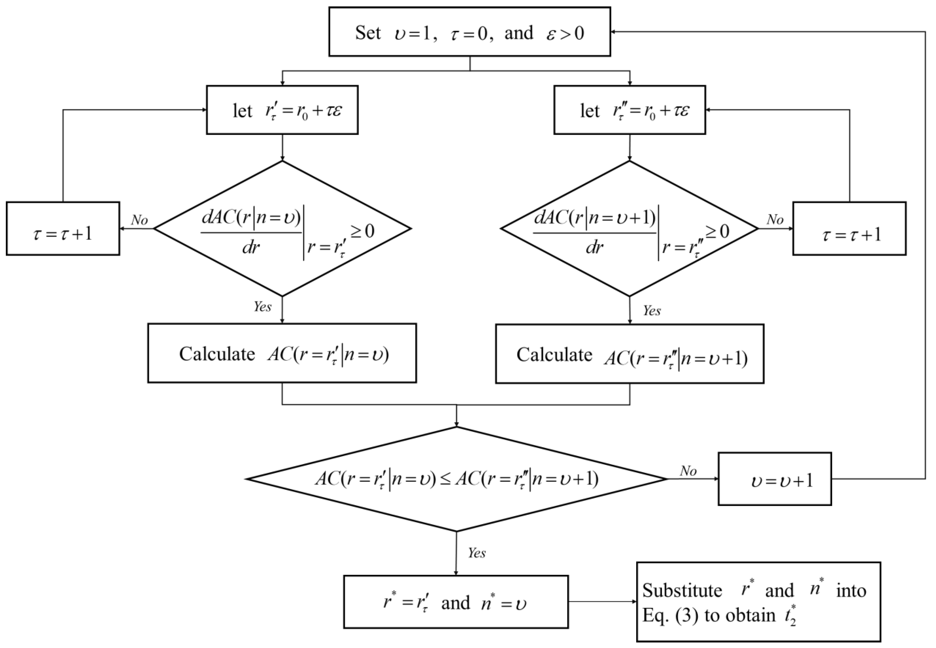
The primary objective of this study is to determine the optimal production, maintenance, and investment strategies to achieve minimal total cost per unit. Equation (3) shows that the value of the t 2 depends on n and r ; hence, the total cost function can be reduced to A C ( n ,   r ) . Because n is a positive integer, we first explore the objective under the given number of maintenance times, i.e., Min   A C ( r n ) . According to the first-derivative test, we observe the pattern of A C ( r n ) during r [ r 0 ,   f r ,   2 / p f θ 2 ) . Under the A C ( r n ) is a convex function of r ; if d A C ( r n ) / d r r = r 0 0 , A C ( r n ) increases during r [ r 0 ,   f r ,   2 / p f θ 2 ) . This implies that the investment of recovery equipment would not be beneficial because the larger value for r results in a higher value of A C ( r n ) . Therefore, the optimal recovery rate is r * = r 0 . If d A C ( r n ) / d r r = r 0 < 0 , and the recovery rate can be increased to r * , which satisfies d A C ( r n ) / d r r = r * = 0 . For the number of maintenance times, we can observe the effect of increasing the times on the value of A C ( r * n ) to determine the optimal times. Based on the above results, Figure 4 plots a simple algorithm procedure for finding the optimal solution ( r * ,   n * ,   t 2 * ) in which the ε > 0 is an accuracy of solution t 2 * . In summary, because the proposed model is a nonlinear integer programming problem with the high-power expression of the polynomial function, it is difficult to provide a theoretical proof to verify the optimal solution. Instead, this study tries to use numerical analysis to verify the convexity of the total cost function.

6. Numerical Example

To exhibit the usability of the proposed model, we quote an application example proposed by Su et al. [12]. They investigated an imperfect production–inventory system involving a pulp and paper manufacturing industry with an inner circular economy, wherein defective products and waste can become scrap returns after passing specific processing in converted equipment. This system manufactures two products with different feed rates of scrap returns, and the lower feed rate takes precedence to enter the production line. Based on Su et al., this study extends their work to survey the maintenance strategy during the out-of-control stage. The values of the parameters pertaining to the imperfect production–inventory system are listed as follows:
  • Demand parameters: d 1 = 400 kg/day and d 2 = 300 kg/day;
  • Production parameters: f n = 100 kg/day, f r ,   1 = 2 kg/day, f r ,   2 = 40 kg/day, p f = 600 kg/day, and t 1 = 3.4799 days. Note that the value of t 1 adopts the estimated results from Su et al. [12];
  • Cost parameters: K c = $1000, C = $10/kg, C p = $5/kg, C r = $2/kg, C l , 1 = $0.15/kg, C l , 2 = $0.10/kg, C m = 50/time, S r = $2 kg/day, S n = $3 kg/day, S f , 1 = $6 kg/day, S f , 2 = $4 kg/day, and λ = $100;
  • Imperfect parameters: θ 1 = 0.1, k = 0.01, and r 0 = 0.1;
  • Accuracy parameter: ε = 10 4 .
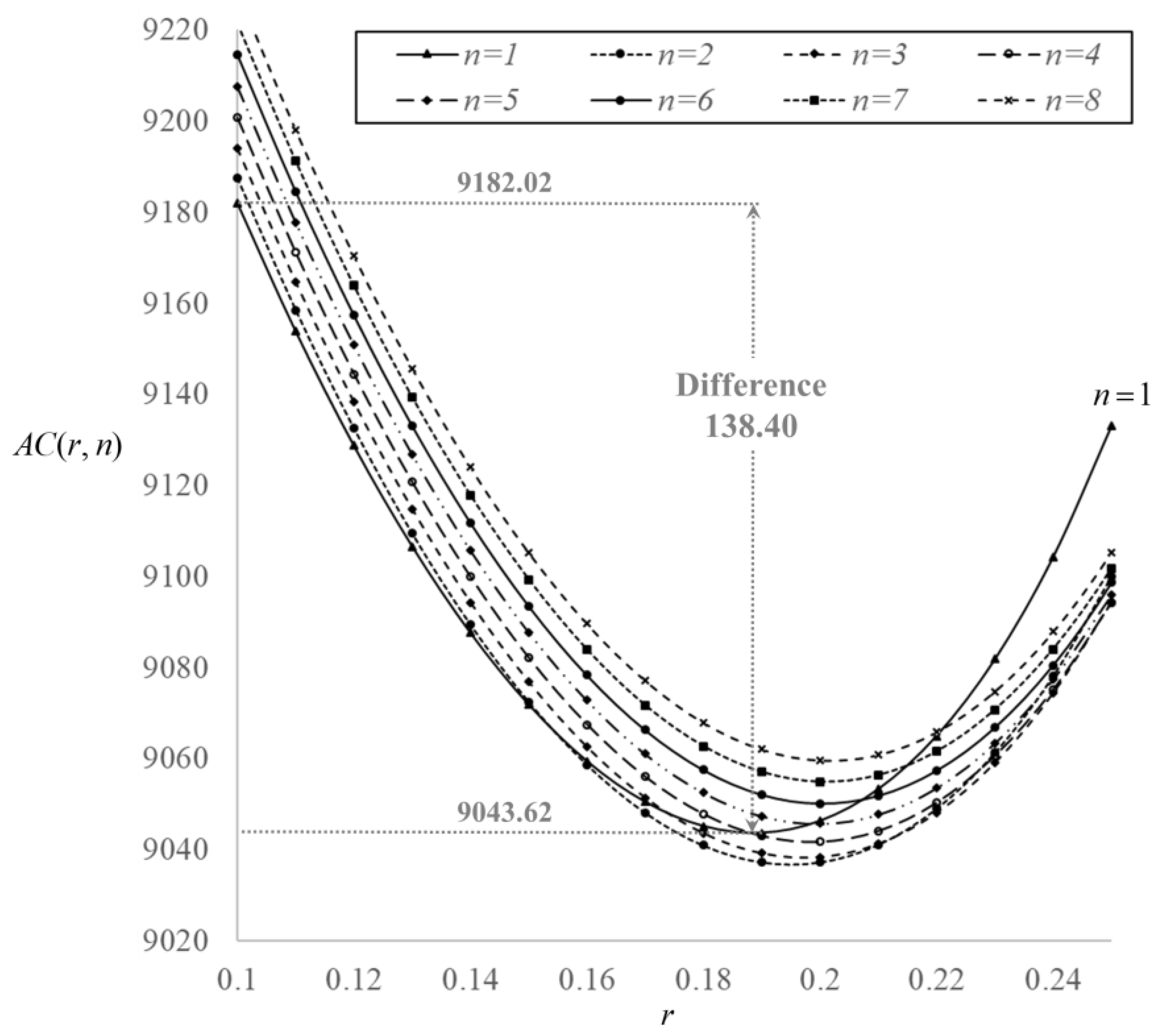
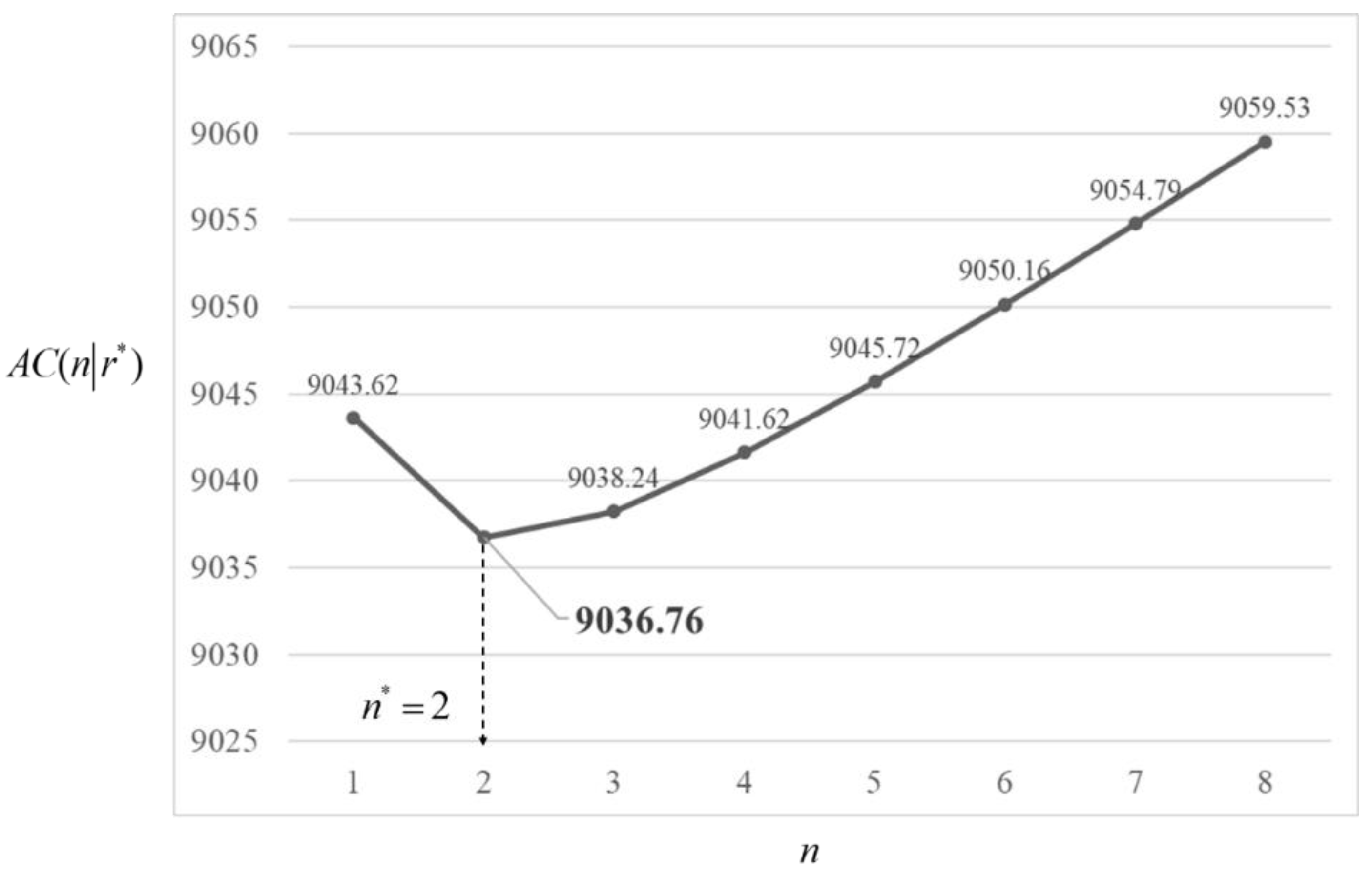
After implementing the proposed algorithm, the optimal solutions can be obtained, i.e., r * = 0.1950, n * = 2, t 2 * = 1.2081, and A C ( t 2 * ,   n * ,   r * ) = 9036.76. Furthermore, the curves of the total cost function with respect to r under different values of n are plotted in Figure 5. Note that these curves are plotted in the feasible solution interval of the recovery rate, r [ r 0 ,   f r ,   2 / p f θ 2 ) . Figure 6 also shows the graphical representation of A C ( n r * ) . From Figure 5 and Figure 6, it is found that the convexity of the total cost function can be verified numerically, which implies that the optimal solutions obtained through the algorithm can ensure the global optimum. In other words, implementing both a circular economy and process maintenance strategies can promote cost control in this numerical example. From Figure 5, it is found that the total cost per unit time is 9182.02 when both circular economy and process maintenance strategies are unimplemented (i.e., our model becomes the traditional EPQ model when n = 1 and r = r 0 = 0.1 ). If the capital investment in recovery capacity improvement is implemented, the total cost per unit time will be saved by 138.40 (i.e., cost from 9182.02 to 9043.62). However, the total cost per unit time can be saved by 145.26 (i.e., cost from 9182.02 to 9036.76) if both capital investment and maintenance activity are implemented. This result is partly similar to that of Darwish and Ben-Day [5]. The difference is that we further take the rework process and scrap returns into consideration at the same time.

7. Sensitivity Analysis and Managerial Insights

To obtain some managerial insights for decision making, this section further performs a sensitivity analysis involving costs based on the above numerical example. That is, we investigate the effects of changes to cost parameters, including K c , C , C l , 1 , C l , 2 , C p , C r , S f , 1 , S f , 2 , S n , S r , λ , and C m , on the values of n * , r * , t 2 * , Q n * , and A C ( t 2 * ,   n * ,   r * ) . This type of parameter is directly related to costs, and, logically, the increase in each cost directly leads to an increase in the total cost. Therefore, this study aims to analyze the impacts of these parameters on the optimal solutions through sensitivity analysis. The goal is to understand the contribution and influence of these parameters on the overall system under their changes. The results of the sensitivity analysis are tabulated, as shown in Table 2. Note that each parameter is changed separately by + 20 % , + 10 % , 20 % , or 10 % . By observing the data trend in Table 2, we can derive the following managerial insights, which could be a guide for decision making:
  • Though the result that increasing the cost parameters will lead to an increase in the total cost is in line with practical intuition, it is found that the total cost per unit time is relatively sensitive to the production and holding costs (i.e., C , S f , 1 , S f , 2 , and S n ). From a business operations perspective, if companies aim to effectively reduce total costs, they should prioritize parameters that exhibit relatively high sensitivity.
  • When considering production-related cost parameters (i.e., K c , C , C p , C r , λ , and C m ), an increase in the cost parameter value leads to higher optimal values of r * and t 2 * . This implies that the manager could lengthen the production cycle to allocate the growth of these costs. Furthermore, the number of maintenance times could simultaneously increase when these costs increase excessively. From Table 2, the number of maintenance times changes from two to three as the production cost increases by 20%. More precisely, the number of maintenance times starts to increase when the production cost increases by 12%. Table 3 also provides information about the other cost parameters related to the upper boundaries of change in the number of maintenance times. The results show that a change in production-related cost has a higher impact on the number of maintenance times. On the other hand, the total cost per unit time is 9182.02 when both strategies are unimplemented. If both strategies are implemented, the total cost per unit can be saved by 150.84, as the parameter λ decreases by 20% (i.e., cost from 9182.02 to 9031.18; the reduction rate is 16.4%). If the parameter C m decreases by 20%, the total cost per unit can be saved by 147.35 (i.e., cost from 9182.02 to 9034.67; the reduction rate is 16.0%). From the above results, although both reduction rates are close, reducing parameter λ may be relatively efficient.
  • Regarding holding cost parameters (i.e., S f , 1 , S f , 2 , S n , and S r ), with the increase in the value of S f , 1 or S r , the optimal values of r * and t 2 * also increase. This implies that the manager could extend the production cycle to control the growth of these kinds of holding costs. For the holding cost of product 1, the upper boundary of change in the number of maintenance times is also shown in Table 3. Note that the effect of the change to a parameter S r on the number of maintenance times is not significant. However, the holding costs of product 2 ( S f , 2 ) and the new material ( S n ) yield opposite results, and even the number of maintenance times decreases. The main reason is that the production of product 2 is in the out-of-control stage involving decision making, and increasing the recovery rate and production time would lead to an increase in inventories of product 2 and new material requirements. This results in the manager having to reduce the length of the production cycle and the number of maintenance times to avoid the excessive growth of holding costs when the values of S f , 2 and S n increase.
  • As for opportunity cost parameters (i.e., C l , 1 and C l , 2 ), the effects of the changes to opportunity costs on the values of optimal solutions and total cost are not significant. This implies that the manager could focus on other high-impact parameters related to production or investment control.

8. Conclusions

Based on Su et al. [12], this paper explored a production–inventory scenario involving an imperfect production system and developed a more general model with both the circular economy and process maintenance activities, which is not presented in previous studies. This system was formulated as a joint EOQ and EPQ model aimed at determining the optimal production run time, purchase quantity of material, number of maintenance times, and recovery rate that would minimize the total cost per unit time. Furthermore, a computational algorithm was provided to effectively find the optimal solutions. Though it is challenging to mathematically prove the existence and uniqueness of the optimal solution, this study utilized numerical and graphical techniques to ensure the optimal solutions obtained through the algorithm were the local optimum. This study also performed numerical and sensitivity analyses on a practical case to provide some managerial insights pertaining to the reference for decision making. First, an optimal combination of circular economy and process maintenance strategies was determined by observing the impact of parameter changes on optimal decisions. In the proposed case, the total cost per unit time can be saved by 145.26 (i.e., reducing the cost from 9182.02 to 9036.76) when both capital investment and process maintenance strategies are implemented in the production system. Second, when the cost-related parameter increases, the capital investment in recovery capacity improvement would be increased first, and the number of maintenance times starts to increase when it increases to a boundary (please see Table 3). Third, enhancing the production cost can significantly decrease the overall cost per unit time. The total cost per unit time can be saved by 997.23 if the unit production cost of the finished product is decreased by 20%. Finally, in terms of holding cost parameters, the total cost per unit time can be effectively reduced by improving the holding cost of product 2 (i.e., a reduction of 4.27% in the total cost can be achieved by reducing the holding cost of product 2 by 20%).
Some research limitations and suggestions for future research can be considered to extend our model. Initially, one can take into account the deteriorating properties of items, such as raw materials and finished products. Second, the maintenance process may be imperfect in practice; that is, the defective rate in the out-of-control stage cannot be adjusted to the in-control stage at each maintenance time. Third, multi-products, multi-materials, and multi-stages can be explored to make the proposed model more applicable to production situations. Fourth, we can consider the impacts of external factors, such as government policy, COVID-19, and international influences, on demand patterns, material procurement, labor, and shipment. Finally, implementing CSR activities (e.g., social donations, environmental protection, green industrial development, etc.) has already been an important topic at present, and it has been confirmed that the financial performance of firms can be improved. Therefore, the effects of CSR activities in the proposed production system can be explored in future research.

Author Contributions

Conceptualization, R.-H.S. and M.-W.W.; methodology, M.-W.W.; software, R.-H.S.; validation, R.-H.S., M.-W.W. and C.-T.Y.; formal analysis, R.-H.S., M.-W.W. and C.-T.Y.; investigation, R.-H.S. and C.-H.H.; resources, R.-H.S. and M.-W.W.; data curation, R.-H.S. and C.-H.H.; writing—original draft preparation, R.-H.S., M.-W.W., C.-T.Y. and C.-H.H.; writing—review and editing, R.-H.S., M.-W.W. and C.-T.Y.; project administration, R.-H.S. and C.-T.Y.; visualization, R.-H.S., M.-W.W. and C.-T.Y. All authors have read and agreed to the published version of the manuscript.

Funding

This work is partially supported by the National Science and Technology Council, Taiwan, under grant numbers NSC 110-2410-H-231-001-MY2 and NSC 111-2410-H-030-027.

Data Availability Statement

Not applicable.

Conflicts of Interest

The authors declare that there are no conflict of interest.

Abbreviations

Parameters
K c The ordering and set-up costs per cycle;
f n The feed rate of new materials;
f r , j The feed rate of scrap returns for a product j , where j = 1 ,   2 ;
p f The production rate of the finished product;
d j The demand rate of the product j , where j = 1 ,   2 ;
θ 1 The defective rate during the in-control stage;
θ 2 The defective rate during the out-of-control stage;
Q r t The maximum stock of scrap returns;
Q f , j The maximum stock of the product j , where j = 1 ,   2 ;
S r The holding cost of scrap returns per unit/per unit time;
S n The holding cost of new material per unit/per unit time;
S f , j The holding cost of product j per unit/per unit time, where j = 1 ,   2 ;
C The production cost of a finished product per unit;
C r The processing cost for converting a defective product to scrap returns;
C l , j The opportunity cost of a defective product j that cannot be converted to scrap returns, where j = 1 ,   2 ;
C p The purchasing cost of new material per unit;
C m The maintenance cost of equipment for recovering an out-of-control stage to an in-control stage in the production line;
t j , d The period during which the stock is depleted for the product j , where j = 1 ,   2 ;
t 1 The production run time during the in-control stage; random variable.
Decision variables
t 2 The production run time during the out-of-control stage;
Q n The purchasing quantity of new material per cycle;
r The recovery rate of scrap returns;
n The number of maintenance times with n 1 .

References

  1. Su, R.H.; Weng, M.W.; Huang, Y.F. Innovative maintenance problem in a two-stage production-inventory system with imperfect processes. Ann. Oper. Res. 2019, 287, 379–401. [Google Scholar] [CrossRef]
  2. Ellen MacArthur Foundation. Towards the Circular Economy: Economic and Business Rationale for an Accelerated Rransition. 2012. Available online: https://ellenmacarthurfoundation.org/topics/circular-economy-introduction/overview (accessed on 11 May 2023).
  3. Nkansah, A.; Attiogbe, F.; Kumi, E. Scrap metals’ role in circular economy in Ghana, using Sunyani as a case study. Afr. J. Environ. Sci. Technol. 2015, 9, 793–799. [Google Scholar]
  4. Paletta, A.; Filho, W.L.; Balogun, A.L.; Foschi, E.; Bonoli, A. Barriers and challenges to plastics valorization in the context of a circular economy: Case studies from Italy. J. Clean. Prod. 2019, 241, 118149. [Google Scholar] [CrossRef]
  5. Darwish, M.A.; Ben-Daya, M. Effect of inspection errors and preventive maintenance on a two-stage production inventory system. Int. J. Prod. Econ. 2007, 107, 301–313. [Google Scholar] [CrossRef]
  6. Pearn, W.L.; Su, R.H.; Weng, M.W.; Hsu, C.H. Optimal production run time for two-stage production system with imperfect processes and allowable shortages. Cent. Eur. J. Oper. Res. 2010, 19, 533–545. [Google Scholar] [CrossRef]
  7. Chang, H.J.; Su, R.H.; Yang, C.T.; Weng, M.W. An economic manufacturing quantity model for a two-stage assembly system with imperfect processes and variable production rate. Comput. Ind. Eng. 2012, 63, 285–293. [Google Scholar] [CrossRef]
  8. Priyan, S.; Mala, P.; Palanivel, M. A cleaner EPQ inventory model involving synchronous and asynchronous rework process with green technology investment. Clean. Logist. Supply Chain 2022, 4, 100056. [Google Scholar] [CrossRef]
  9. Paul, S.K.; Sarker, R.; Essam, D. A disruption recovery plan in a three-stage production-inventory system. Comput. Oper. Res. 2015, 57, 60–72. [Google Scholar] [CrossRef]
  10. Wang, Z.; Chan, F.T.S. A Robust Production Control Policy for a Multiple-Stage Production System with Inventory Inaccuracy and Time-Delay. In Proceedings of the 2013 IEEE International Conference on Automation Science and Engineering (CASE 2013), Madison, WI, USA, 17–20 August 2013. [Google Scholar]
  11. Su, R.H.; Weng, M.W.; Yang, C.T. Effects of corporate social responsibility activities in a two-stage assembly production system with multiple components and imperfect processes. Eur. J. Oper. Res. 2020, 293, 469–480. [Google Scholar] [CrossRef]
  12. Tayyab, M.; Sarkar, B.; Yahya, B.N. Imperfect multi-stage lean manufacturing system with rework under fuzzy demand. Mathematics 2019, 7, 13. [Google Scholar] [CrossRef] [Green Version]
  13. Wang, A.; Shi, J. Holistic modeling and analysis of multistage manufacturing processes with sparse effective inputs and mixed profile outputs. IISE Trans. 2020, 53, 582–596. [Google Scholar] [CrossRef]
  14. Cui, P.H.; Wang, J.Q.; Li, Y. Data-driven modeling, analysis and improvement of multistage production systems with predictive maintenance and product quality. Int. J. Prod. Res. 2021, 22, 6848–6865. [Google Scholar]
  15. Öztürk, H. Modeling an inventory problem with random supply, inspection and machine breakdown. Opsearch 2019, 56, 497–527. [Google Scholar] [CrossRef]
  16. Öztürk, H. Optimal production run time for an imperfect production inventory system with rework, random breakdowns and inspection costs. Oper. Res. 2021, 21, 167–204. [Google Scholar] [CrossRef]
  17. Dey, B.K.; Pareek, S.; Tayyab, M.; Sarkar, B. Autonomation policy to control work-in-process inventory in a smart production system. Int. J. Prod. Res. 2021, 59, 1258–1280. [Google Scholar] [CrossRef]
  18. Dey, B.K.; Sarkar, B.; Sarkar, M.; Pareek, S. An integrated inventory model involving discrete setup cost reduction, variable safety factor, selling price dependent demand, and investment. RAIRO Oper. Res. 2019, 53, 39–57. [Google Scholar] [CrossRef] [Green Version]
  19. Huang, H.; He, Y.; Li, D. Coordination of pricing, inventory, and production reliability decisions in deteriorating product supply chains. Int. J. Prod. Res. 2018, 56, 6201–6224. [Google Scholar] [CrossRef]
  20. Manna, A.K.; Das, B.; Tiwari, S. Impact of carbon emission on imperfect production inventory system with advance payment base free transportation. RAIRO Oper. Res. 2020, 54, 1103–1117. [Google Scholar] [CrossRef] [Green Version]
  21. Su, R.H.; Weng, M.W.; Yang, C.T.; Li, H.T. An imperfect production–inventory model with mixed materials containing scrap returns based on a circular economy. Processes 2021, 9, 1275. [Google Scholar] [CrossRef]
  22. Sarkar, S.; Shewchuk, J.P. Use of advance Demand Information in multi-stage production-inventory systems with multiple demand classes. Int. J. Prod. Res. 2013, 51, 57–68. [Google Scholar] [CrossRef]
  23. Mahata, G.C. A production-inventory model with imperfect production process and partial backlogging under learning considerations in fuzzy random environments. J. Intell. Manuf. 2014, 28, 883–897. [Google Scholar] [CrossRef]
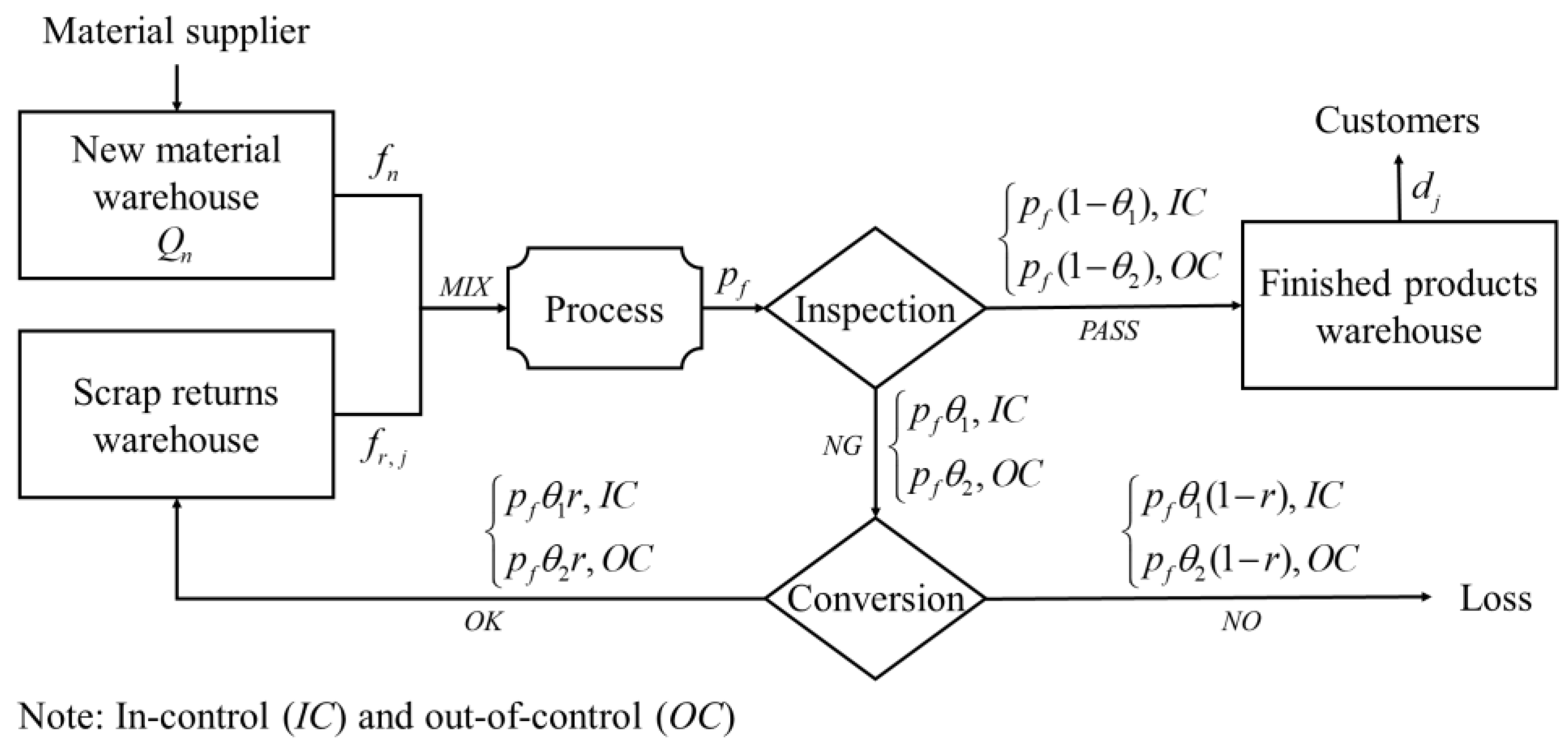
Figure 1. Imperfect production system with the conversion process.
Mathematics 11 03041 g001
Figure 2. The change in defective rate during a cycle.
Mathematics 11 03041 g002
Figure 3. The patterns of inventory levels.
Mathematics 11 03041 g003
Figure 4. The procedure of the proposed algorithm.
Mathematics 11 03041 g004
Figure 5. The curves of the total cost per unit time with r for n = 1 ( 1 ) 8 .
Mathematics 11 03041 g005
Figure 6. The graphical representation of A C ( n r * ) .
Mathematics 11 03041 g006
Table 1. Comparison of the major issues of existing EPQ models with the present paper.
ReferencesSingle/Multiple StageImperfect ProcessRework ProcessScrap ReturnsMaintenance
Darwish and Ben-Daya [5]MultipleRS V
Pearn et al. [6]MultipleCDV
Chang et al. [7]MultipleCDV
Sarker and Shewchuk [22]MultipleRDV
Paul et al. [9]MultipleRDV
Su et al. [1]MultipleCDV
Su et al. [11]MultipleCDV
Tayyab et al. [12]MultipleRSV
Öztürk [15]SingleRB
Öztürk [16]SingleRBV V
Dey et al. [17]SingleRD/RSV
Dey et al. [18]SingleRS
Huang et al. [19]SingleRS V
Manna et al. [20]SingleRSV
Mahata [23]SingleRSV
Su et al. [21]MultipleRSVV
This paperMultipleRSVVV
Note: constant defective rate (CD), random defective rate (RD), random machine breakdowns (RB), random state shift (RS).
Table 2. Sensitivity analysis for cost parameters.
ParameterChange
(%)
Change in
n * r * t 2 * Q n * A C ( t 2 * ,   n * ,   r * )
K c 202 0.1981 1.2402 472.0100 9071.29 (+0.38%)
102 0.1966 1.2242 470.4100 9054.07 (+0.19%)
−102 0.1935 1.1919 467.1800 9019.35 (−0.19%)
−202 0.1918 1.1757 465.5600 9001.85 (−0.39%)
C 203 0.2256 1.5375 501.7400 9995.42 (+10.61%)
102 0.2098 1.3657 484.5600 9520.64 (+5.35%)
−102 0.1783 1.0426 452.2500 8543.59 (−5.46%)
−202 0.1590 0.8673 434.7200 8039.53 (−11.04%)
C l , 1 202 0.1951 1.2092 468.9140 9037.63 (+0.01%)
102 0.1951 1.2087 468.8590 9037.19 (+0.00%)
−102 0.1950 1.2076 468.7470 9036.32 (−0.00%)
−202 0.1949 1.2070 468.6920 9035.88 (−0.01%)
C l , 2 202 0.1950 1.2081 468.7950 9036.87 (+0.01%)
102 0.1950 1.2081 468.7990 9036.81 (+0.01%)
−102 0.1950 1.2082 468.8070 9036.70 (−0.00%)
−202 0.1950 1.2082 468.8110 9036.64 (−0.00%)
C p 202 0.1976 1.2349 471.4810 9118.01 (+0.90%)
102 0.1963 1.2216 470.1450 9077.42 (+0.45%)
−102 0.1937 1.1947 467.4560 8996.03 (−0.45%)
−202 0.1924 1.1811 466.1030 8955.25 (−0.90%)
C r 202 0.1961 1.2187 469.8630 9054.06 (+0.19%)
102 0.1955 1.2134 469.3330 9045.41 (+0.10%)
−102 0.1945 1.2028 468.2730 9028.09 (−0.10%)
−202 0.1940 1.1975 467.7430 9019.41 (−0.90%)
S f , 1 202 0.2148 1.4216 490.1450 9267.00 (+2.55%)
102 0.2053 1.3168 479.6730 9153.84 (+1.30%)
−102 0.1837 1.0950 457.4850 8915.29 (−1.34%)
−202 0.1712 0.9767 445.6579 8788.90 (−2.74%)
S f , 2 201 0.1315 0.6431 412.3048 9303.05 (+2.95%)
102 0.1664 0.9332 441.3092 9185.70 (+1.65%)
−103 0.2245 1.5246 500.4450 8858.75 (−1.97%)
−203 0.2507 1.8530 533.2880 8650.57 (−4.27%)
S n 202 0.1921 1.1780 465.7870 9151.05 (+1.26%)
102 0.1935 1.1929 467.2790 9093.94 (+0.63%)
−102 0.1965 1.2237 470.3600 8979.49 (−0.63%)
−202 0.1981 1.2396 471.9520 8922.13 (−1.27%)
S r 202 0.1952 1.2099 468.9770 9045.76 (+0.10%)
102 0.1951 1.2090 468.8900 9041.26 (+0.05%)
−102 0.1949 1.2073 468.7160 9032.26 (−0.05%)
−202 0.1949 1.2064 468.6300 9027.75 (−0.10%)
λ 202 0.1931 1.1889 466.8750 9042.20 (+0.06%)
102 0.1941 1.1985 467.8350 9039.49 (+0.03%)
−102 0.1960 1.2179 469.7790 9033.99 (−0.03%)
−202 0.1969 1.2277 470.7640 9031.18 (−0.06%)
C m 202 0.1952 1.2101 468.9970 9038.84 (+0.02%)
102 0.1951 1.2091 468.9000 9037.80 (+0.01%)
−102 0.1949 1.2072 468.7060 9035.72 (−0.01%)
−202 0.1948 1.2062 468.6090 9034.67 (−0.02%)
Table 3. Boundaries of change in the number of maintenance times.
Parameter K c C C p C r λ C m S f , 1
Boundary139.5%12.0%143.6%220.5%499.7%160.9%20.3%
Disclaimer/Publisher’s Note: The statements, opinions and data contained in all publications are solely those of the individual author(s) and contributor(s) and not of MDPI and/or the editor(s). MDPI and/or the editor(s) disclaim responsibility for any injury to people or property resulting from any ideas, methods, instructions or products referred to in the content.