Algebraic-Connectivity-Based Multi-USV Distributed Formation Method via Adding a Reverse Edge

Abstract

This paper concerns the formation problem in multi-USV cluster formation containment tracking tasks with a special topology. A topology reconstruction method was proposed that enables the followers’ formation to be dispersed while achieving the fastest convergence rate for the system. This topology structure is based on tree topology and DAG (directed acyclic graph) local structure stem as prototypes, using the principle of adding reverse edges on the stem to reduce algebraic connectivity. By adding a reverse edge to obtain a more dispersed formation, a method for selecting appropriate reverse edges was achieved. Through relevant theoretical quantitative and qualitative analysis, it was demonstrated that adding this reverse edge can enable the system to achieve the fastest convergence rate. Finally, through simulation experiments, it was verified that the selected reverse edge can optimize the formation of followers and achieve the fastest convergence rate.

1. Introduction

The collaborative control of multi-unmanned surface vehicle (USV) systems has been increasingly applied in military fields in recent years, such as coordinated escort, coordinated mine sweeping, and coordinated encirclement of enemy ships [1]. Similarly, in civilian fields, it can expand the scope of marine operations, improve operational efficiency, and complete complex tasks that cannot be achieved by a single ship, including coordinated search and rescue, coordinated reconnaissance, long-distance supply, maritime patrol, and coordinated transportation, among others. The formation problem is an important issue in the control of multi-USV systems [2,3,4], which requires USVs to maintain a certain relative spatial position while in motion. This plays an important role when USV clusters complete common tasks such as oil and gas exploration and maritime search and rescue [5].

The field of formation control application is broad, which has led to its rapid development [6,7,8]. Formation control can be classified into two types of problems [9] based on whether the formation spatial position changes over time: (1) formation problem, which controls multiple agents to achieve a pre-specified formation that does not change over time, and (2) formation tracking problem, which requires agents to track a pre-specified formation trajectory that may change over time. In this case, the formation may also change over time, and changing the formation based on actual motion trajectory is a more practical approach. Several commonly used formation methods include the leader-following method [10], behavior-based method [11], virtual structure method [12], etc. A unified formation method framework based on consensus for second-order multi-agent systems was proposed in reference [13], which makes the aforementioned formation methods special cases of this framework. The leader-following method combined with the line-of-sight (LOS) strategy has been used to study the safety formation problem of multi-USV systems considering unmodeled dynamics, environmental disturbances, input saturation, and output constraints [14]. In actual complex maritime missions, such as cooperative surveillance, it is not enough to have multiple USVs tracking a target. Usually, multiple leader USVs form a safe area through formation, and USV followers enter the area to execute hazardous tasks [15]. The USV leaders maintain the desired formation, and the follower USVs converge to the convex hull formed by the leader USVs. This problem is known as the formation containment problem [16]. The leaders’ formation can be controlled by setting the distance and angle between the leader and the target from the shore, while the follower’s formation is controlled by the leader, and its relative position in the convex hull cannot be directly determined. However, for safety and the efficient completion of various tasks, the position of the follower in the convex hull is essential. Due to the constraints of the containment control law, the formation of the followers cannot be arbitrarily set by the control protocol. To design a formation for the followers, a topology structure can be used. Reference [17] proved that the topology network enables the followers of the multi-agent system to converge to the convex hull and maintain a convex combination of some leader’s formation within the convex hull; based on this theory, two kinds of follower regular polygon formations were designed. However, to our knowledge, the relevant problems of designing formations to make the system have convergence rate advantages have not been widely studied.

In the problem of formation containment of cooperative control of multiple USVs, saving communication cost has significance. Reference [18] applies a dynamic event-triggered mechanism (DET) to the formation containment-tracking control of discrete multi-agent systems, saving communication cost and communication resource utilization. In addition to the event-triggered method to improve communication bandwidth utilization, communication resource utilization can also be improved by designing communication topology [17], and simplifying the communication link between USVs can also play a role in improving communication resource utilization [17]. Therefore, this article selects a low communication resource connection method with a simple structure, low cost, and high effectiveness, tree topology [19,20], as the communication connection topology between various levels of USVs.

Due to its advantages such as short communication line length, low cost, ease of node expansion, convenient search, and isolation of fault paths [19,21,22], tree topology networks are often used in the topology structure of tracking and formation control for various multi-agent system clusters [23,24]. Moreover, the tree topology structure is also a directed acyclic graph (DAG).

A directed acyclic graph (DAG) is a kind of directed graph with topological order and no directed cycle. Algebraic connectivity is a crucial index in graph theory and is defined as the smallest non-zero eigenvalue of the Laplacian matrix of the communication topology of a multi-agent system [25,26]. In the containment problem of multiple USVs, if there are multiple follower USVs in the convex hull, their algebraic connectivity is often related to the degree of formation density of the follower USVs in the convex hull; the larger the algebraic connectivity, the denser the follower USVs. In more complex and harsh actual sea areas, if the formation of follower USVs in the convex hull is too dense, it is easy to cause collisions between agents, and it is not conducive to obstacle avoidance, so the formation of followers in the convex hull should be as dispersed and sparse as possible. Therefore, a relatively small algebraic connectivity is needed when forming a formation for the follower USVs. In addition, algebraic connectivity can also reflect the convergence rate of the collaborative multi-USV system [27,28]. When the formation of follower USVs guarantees relative dispersion and safety, it is best to have the fastest possible convergence rate.

Adding a reverse edge on a DAG may decrease its algebraic connectivity [28,29,30]. However, there is currently no effective and intuitive standard for judging whether adding a reverse edge to a general DAG affects its algebraic connectivity [28]. Nevertheless, some general rules that affect the convergence rate have been summarized for some special DAGs, such as 1D chains and 2D grids of geographic areas commonly used in mobile ad hoc networks (MANETs) in the communication field [31,32]. The interference of the reverse edge depends only on the reverse range, but it is independent of the specific location of the reverse edge in the graph and the size of the graph [30]. For DAGs with nodes of in-degree 1, reference [28] defines a reverse coefficient to determine whether a reverse edge is an interfering edge by comparing it with one through calculation. Reference [29] defined a single-chain DAG local structure as a stem; for example, the DAG in Figure 1, a local structure like $(5,6,7,8)$ is a stem.

The reference presented an accurate condition for the interference reverse edge of this structure, took the dominant convergence rate as a function, and quantitatively studied its monotonic relationship with the reverse range nodes’ in-degree. In addition, due to the stem presenting a network structure with a single-chain topology with topological order, as a relatively simple and connected topology, it has advantages such as simplicity, reliability, and low latency in communication, making it suitable for small and rapidly deployable networks [33,34,35,36,37], such as the USV communication network. Therefore, it can be used for communication topology connection between followers in multi-USV system cooperative tasks.

Inspired by the above studies, this paper designed a special type of DAG communication topology network for USV clusters based on the tree-like topology structure, which is advantageous in saving communication costs. The algebraic connectivity of the communication topology was also taken into consideration, and a topology reconstruction method based on reverse edge was proposed for optimizing the formation of followers in the formation containment tracking problem. Specifically, this paper has achieved the following:

(1)

A simple form of a USV (unmanned surface vehicle) follower network is considered in this article, and a stem structure is used to describe the communication topology between followers. As the algebraic connectivity would be decreased by adding a reverse edge to the stem structure, this property is utilized by this article to add a communication link to USV followers in order to reduce the algebraic connectivity, thereby making the follower formations more dispersed and more conducive to USV distributed security operations.

(2)

The changes in algebraic connectivity by adding different reverse links to the stem-structured communication topology of the USV follower cluster are analyzed in this article. A method for optimal addition of a reverse link is proposed based on the above rules, considering the appropriate algebraic connectivity of the communication topology, in order to optimize the problem of slower convergence rate caused by adding a reverse link to the stem structure. The formation of the USV followers is improved by this method while minimizing the loss of convergence rate to the convex hull of the leaders.

(3)

Compared to the more complex topology reconstruction methods that require extensive changes to the communication links, the advantage of the method described in this article is that it only involves minor modifications to the original DAG graph, i.e., adding a reverse edge to the stem structure, which can significantly change the formation of USV followers while ensuring a good convergence rate.

The structure of the rest of this paper is as follows: Section 2 presents some preliminary knowledge to support the conclusion. Section 3 proposes a method of adding reverse edges for a special class of communication topologies to make the formation of multiple USVs more dispersed, while minimizing the convergence rate of system loss. Section 4 conducts some simulation experiments. Finally, Section 5 presents the conclusion of this paper.

2. Prelimination and Problem Formulation

2.1. Graph Theory Stem and Reverse Edge

Consider a network with a number of nodes $N>2$, represented by a directed graph $\mathcal{G}=(\mathcal{V},\mathcal{E},\mathcal{T})$. Here, $\mathcal{V}=\left\{v_1,\dots ,v_N\right\}$ is the set of nodes, $\mathcal{E}\subset \mathcal{V}\times \mathcal{V}$ is the set of edges, $\mathcal{T}$ is the adjacency matrix, and its $(i,j)$ element $a_{ij}\in \{0,1\}$. In particular, the existence of an edge from node j to node i is represented as $a_{ij}=1$, and its absence is represented as $a_{ij}=0$. Additionally, this article assumes that there are no circular connections where a node is connected to itself, i.e., $a_{ii}=0,i=1,\dots ,N$. The in-degree of node $v_i$ is defined as ${deg}_{in}\left(v_i\right)={\displaystyle \sum _{j=1}^N}{a}_{ij}$. Let $\mathcal{D}=\mathrm{diag}\left\{{deg}_{in}\left(v_1\right),{deg}_{in}\left(v_2\right),\dots ,{deg}_{in}\left(v_N\right)\right\}$ represent the in-degree of graph G.${deg}_{in}\left(v_i\right)$ represent the in-degree of the node $v_i$, in-degree means the number of the agents that connect agent $v_i$. All other off-diagonal elements are 0. The Laplacian matrix of graph G is defined as $L=\mathcal{D}-\mathcal{T}$.

The state represented as a single agent object is described by the following expression for the state of all agents in the network, since there are N agents in the entire network. The $x_i\left(t\right)\in R^2$ in this paper means the USV i position coordinates:

$${\dot{x}}_i=-\sum _{i=1}^N{a}_{ij}\left(x_j-x_i\right)$$

(1)

where $i\in [1,2,\dots ,N]$. Writing the equation in vector form yields:

$$\dot{x}=-Lx$$

(2)

In order for individual agents to achieve what is known as consensus, they need to be part of a connected network. The simplest requirement for a connected network is that it has a spanning tree. That is, if a directed graph has a root node with directed paths to all other nodes, the directed graph is said to contain a spanning tree.

In addition, the matrix L has an eigenvector ${[1,1,\dots ,1]}^T$ with a non-negative eigenvalue, and the smallest eigenvalue is 0. The non-zero smallest eigenvalue is called the algebraic connectivity, which has rich meanings in specific application contexts.

Definition 1

([30]). For a network with a directed graph that contains a spanning tree, the minimum real part of the non-zero smallest eigenvalue of its Laplacian matrix, i.e., $\Re \left({\lambda }_2\left(L\right)\right)$, is called the dominant convergence rate, if all eigenvalues have real parts.

Below, we introduce a special network structure called DAG (directed acyclic graph).

Definition 2

([31]). DAG is a directed graph without directed cycles. It consists of a set of nodes and a set of edges, where each edge connects one node to another, ensuring that there is no node i that can start from a series of edges and eventually loop back to i.

Definition 3

([29]). Every DAG always has a topological ordering, which is a sequence of nodes where the starting node of each edge comes before its ending node. A topological ordering is only possible for a graph if it is a DAG. However, in general, this ordering is not unique.

Typical examples of DAGs include singly linked chains, grids, trees, mushrooms, etc. Among them, there is a local DAG structure called stem, which has a singly linked network structure and is located in a local region of a large network. More importantly, it can be used for local quantitative analysis and can reduce the workload of analyzing large networks.

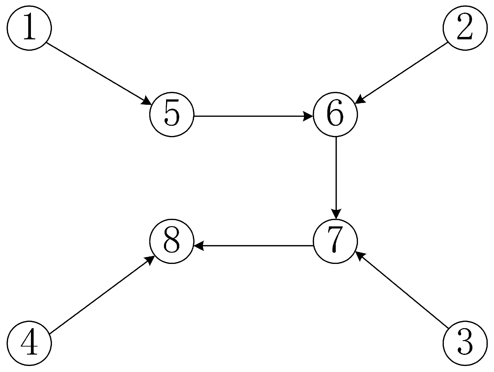
Remark 1.

The following graph in Figure 2 is a directed acyclic graph (DAG) with topological ordering. The ordering refers to the sequence of the nodes, ensuring that for each edge, the start node always precedes the end node. One topological ordering of a graph is $(A,C,E,B,D)$.

Definition 4

([30]). For a DAG with a topological ordering of N nodes, suppose there is a path from node ℏ to node ℓ and $\ell >\hslash$. If there is no edge from i to j and $|i-j|\ge 2$, $i,j\in [\hslash ,\ell ]$, the number of nodes on the stem, i.e., $\ell -\hslash +1$, is called the length of the stem. Nodes ℏ and ℓ are, respectively, called the start node and end node, and the ordered set of nodes from the start node to the end node according to the topological ordering is called the reverse range.

Remark 2.

The following graph in Figure 1 is a directed acyclic graph. For example, $(5,6,7,8)$ is a stem structure, where start node $\hslash =5$ and the end node $\ell =8$. Choose any $i,j$: $i,j\in [5,8]$, and $|i-j|\ge 2$. The possible values for $(i,j)$ are as follows: $(5,7),(5,8),(6,8),(7,5),(8,5),$ and $(8,6)$. By definition, there is no direct edge from i to j in the graph. Therefore, $(5,6,7,8)$ is a stem structure.

The greatest advantage of the stem structure lies in its ability to perform both quantitative and qualitative analyses, as stated in the following lemma:

Lemma 1

([30]). Consider a graph with N nodes and a topological ordering, where the Laplacian matrix is a lower triangular matrix. Assume that the graph has a stem with a start node h and another node l, with $r=l-h>0$. The in-degree requirements for all nodes in the stem structure are as follows:

• The in-degree of node h is $d_0\ge 1$.
• The in-degree of node l is $d_{+}\ge 1$.
• The in-degrees of nodes from $h+1$ to $l-1$ form a set $D=\left\{d_i|d_i\ge 1,i=1,\dots ,m\right\}$, where $1\le m\le l-1$. In this sense, there are $r_i\ge 1$ nodes with an incoming degree of $d_i$, for $i=1,\dots ,m$, satisfying ${\sum }_{i=1}^m{r}_i=r-1$. The following relationships hold:

$$d_{+}\le d_0,d_1,d_2,\dots ,d_m,$$

(3)

The impact of adding a reverse edge from node l to node h is as follows:

(1) 

Only $r+1$ eigenvalues in the Laplacian matrix are changed, and the remaining $N-r-1$ eigenvalues remain unchanged.

(2) 

The $r+1$ changed eigenvalues are determined by the following polynomial equations:

$$(\lambda -d_{+})(\lambda -d_0-1)\prod _{i=1}^m{(d_i-\lambda )}^{r_i}=1$$

(4)

The equations always have a real root $\lambda ={\lambda }_{min}\in (d_{+}-1,d_{+})$. In particular, ${\lambda }_{min}$ can be explicitly expressed as ${\lambda }_{min}(d_0,d_1,\dots ,d_m,r_1,\dots ,r_m)$.

(3) 

${\lambda }_{min}$ is smaller than the remaining r roots in Equation (4).

(4) 

For $i=0,1,\dots ,m$, when all other independent variables are fixed, the function ${\lambda }_{min}(d_0,d_1,\dots ,d_m,r_1,\dots ,r_m)$ is strictly monotonically increasing with respect to the independent variable $d_i$.

(5) 

For $i=0,1,\dots ,m$, when other independent variables are fixed, if $d_i\ge 2$, the function ${\lambda }_{min}(d_0,d_1,\dots ,d_m,r_1,\dots ,r_m)$ is strictly monotonically increasing with respect to the independent variable $r_i$. If $d_i=1$, then the function ${\lambda }_{min}(d_0,d_1,\dots ,d_m,r_1,\dots ,r_m)$ is strictly monotonically decreasing with respect to the independent variable $r_i$.

(6) 

If $d_{+}=1$, then ${\lambda }_{min}\in (0,1)$ is the dominant convergence rate.

2.2. The Formation Containment Tracking Control and USV Model

Below is an introduction to the basic description of formation containment tracking tasks. This task essentially divides the multi-agent system into three roles: the tracking leader is responsible for determining the macroscopic motion trajectory of the entire system, the formation leader is responsible for tracking the tracking leader according to the formation set by the motion control protocol, and the followers converge into the convex hull formed by the formation leader according to the motion control protocol.

The main content of this section is to provide motion control protocols for both the formation leader and followers based on the kinematic descriptions of the three roles mentioned above, i.e., Equations (11) and (12). The parameters of the control protocols are determined according to Algorithm 1 in reference [16]. This paper only uses this method to design control protocols.

In order to complete the formation containment tracking tasks, the communication connection methods for USVs with different roles have the following requirements.

Assumption 1

([16]). The communication topology between the tracking leader and the formation leader satisfies the following conditions: it includes a spanning tree, and the root of the tree is the tracking leader.

Assumption 2

([16]). The topology relationship between the formation leader and the followers satisfies the following condition: for any follower, there is at least one formation leader that has a directed path to it.

Considering the entire multi-USV system, according to the order of one tracking leader, N formation leaders, and M followers, the Laplacian matrix can be divided into $L=\left[\begin{array}{ccc}0& 0_{1\times N}& 0_{1\times M}\\ L_{12}& L_{11}& 0_{N\times M}\\ 0_{M\times 1}& L_2& L_3\end{array}\right]$, where $L_{12}\in {\mathrm{R}}^{N\times 1}$, $L_{11}\in {\mathrm{R}}^{N\times N}$, $L_2\in {\mathrm{R}}^{M\times N}$, $L_3\in {\mathrm{R}}^{M\times M}$.

Based on Assumptions 1 and 2, there exists a diagonal matrix $D_l=\mathrm{diag}\left\{d_1,d_2,\dots ,d_N\right\}$ such that $d_i>0(j=1,2,\dots ,N)$ and ${\Phi }_l=D_l{L}_{11}+L_{11}^T{D}_l>0$. There also exists a diagonal matrix $G_f=\mathrm{diag}\left\{g_1,g_2,\dots ,g_M\right\}$ such that $g_j>0(j=1,2,\dots ,M)$ and ${\Xi }_f=G_f{L}_3+L_3^T{G}_f>0$. Feasible matrices $D_l$ and $G_f$ can be calculated as ${\left[d_1,d_2,\dots ,d_N\right]}^T={\left(L_{11}^T\right)}^{-1}{\mathbf{1}}_N$ and ${\left[g_1,g_2,\dots ,g_M\right]}^T={\left(L_3^T\right)}^{-1}{\mathbf{1}}_M$. When applied to a multi-USV system, due to the fact that the research object of this paper is small unmanned boats, and the spatial distance between each USV in the formation is much greater than the length of the USV itself, the motion angle deviation of each USV can be ignored. Therefore, an approximate first-order linear point-mass motion model can be used to describe each USV.

The dynamic descriptions of the formation leaders and followers are as follows:

$$\begin{array}{c}\hfill {\dot{x}}_i\left(t\right)=A{x}_i\left(t\right)+B{u}_i\left(t\right),i=1,2,\dots ,N+M\end{array}$$

(5)

where the position coordinates of the single USV is represented by $x_i\left(t\right)\in {\mathrm{R}}^n$ and $u_i\left(t\right)\in {\mathrm{R}}^m$ as the control input. The dynamic description of the tracking leader USV is given by:

$${\dot{x}}_0\left(t\right)=A{x}_0\left(t\right)+B{r}_0\left(t\right)$$

(6)

where $x_0\left(t\right)\in {\mathrm{R}}^n$ represents the position coordinates of the tracking leader USV, and $r_0\left(t\right)\in {\mathrm{R}}^m$ represents the control input. The time-varying non-zero control input $r_0\left(t\right)$ is unknown to all the formation leaders and followers.

Assumption 3.

The position control input of the tracking leader $r_0\left(t\right)$ is bounded, and there exists a positive real number γ such that $\left|r_0\left(t\right)\right|\le \gamma$.

The expected time-varying formation for the formation leader is given by $h_L\left(t\right)={\left[h_1^T\left(t\right),h_2^T\left(t\right),\dots ,h_N^T\left(t\right)\right]}^T$, where $h_i\left(t\right)$ is piecewise continuously differentiable, which requires that $h_i\left(t\right)$ and ${\dot{h}}_i\left(t\right)$ are both bounded.

$$\begin{array}{c}\hfill {\lim }_{t\to \infty }\left(x_i\left(t\right)-h_i\left(t\right)-x_0\left(t\right)\right)=0,i=1,2,\dots ,N\end{array}$$

(7)

The followers should converge to the convex hull formed by the formation leader, and there exists a set of non-negative numbers ${\beta }_{kj}(j=1,2,\dots ,N)$ such that ${\displaystyle \sum _{j=1}^N}{\beta }_{kj}=1$. The specific convergence position satisfies the following equation.

$$\begin{array}{c}\hfill {\lim }_{t\to \infty }\left(x_k\left(t\right)-\sum _{j=1}^N{\beta }_{kj}{x}_j\left(t\right)\right)=0,k=N+1,N+2,\dots ,N+M\end{array}$$

(8)

The time-varying formation tracking position error between a formation leader and its neighbors is defined as:

$$\begin{array}{c}\hfill {\xi }_i\left(t\right)=a_{i0}\left(x_i\left(t\right)-h_i\left(t\right)-x_0\left(t\right)\right)+\sum _{j=1}^N{a}_{ij}\left((x_i\left(t\right)-h_i\left(t\right))-(x_j\left(t\right)-h_j\left(t\right))\right)\end{array}$$

(9)

where $a_{i0}>0$ if the neighbor of the formation leader includes the tracking leader; otherwise, $a_{i0}=0$.

For the follower, the relative error between itself and its neighbors is defined as:

$${\zeta }_i\left(t\right)=\sum _{j=1}^{N+M}{a}_{ij}\left(x_i\left(t\right)-x_j\left(t\right)\right)$$

(10)

Consider the following formation containment tracking control protocol:

$$\begin{array}{c}\hfill u_i\left(t\right)=v_i\left(t\right)+K_1{\xi }_i\left(t\right)-\eta \widehat{f}\left({\xi }_i\left(t\right)\right),i=1,2,\dots ,N\end{array}$$

(11)

$$\begin{array}{c}\hfill u_i\left(t\right)=K_2{\zeta }_i\left(t\right)-\mu \widehat{f}\left({\zeta }_i\left(t\right)\right),i=N+1,N+2,\dots ,N+M\end{array}$$

(12)

where $v_i\left(t\right)\in {\mathrm{R}}^m(i\in 1,2,\dots ,N)$ represents the time-varying formation tracking compensation input determined by $h_L\left(t\right)$. $K_1\in {\mathrm{R}}^{m\times n}$ and $K_2\in {\mathrm{R}}^{m\times n}$ are constant gain matrices, $\eta$ and $\mu$ are positive constants, and $\widehat{f}\left(\right)$ is a nonlinear function.

2.3. Topology Design

Due to the fact that neither Assumption 1 nor Assumption 2 require any specific topology between the tracking leader and the followers, in general, the tracking leader will not be connected to the followers. As for the topology between the tracking leader and the formation leader, only a spanning tree with the tracking leader as the root is required, and the formation leader’s formation, i.e., the relative position between the formation leader and the tracking leader, is determined by designing the relative position and other parameters in the control protocol. Therefore, in the third part of this paper, the topology between the tracking leader and the formation leader is ignored, and only the topology between the formation leader and the followers is designed.

Assuming that the graph to be considered is composed of leaders with indices 1, 2, …, M and followers with indices M + 1, M + 2, …, N, and their connection satisfies Assumption 2, the Laplacian matrix of the graph becomes $L=\left[\begin{array}{cc}0& 0\\ L_2& L_3\end{array}\right]\in {\mathrm{R}}^{(M+N)\times (M+N)}$, where $L_2\in {\mathrm{R}}^{N\times M}$ and $L_3\in {\mathrm{R}}^{N\times N}$.

Then, the followers will converge to the convex hull formed by the formation leaders, and the specific convergence position is given by the following two lemmas.

Lemma 2

([9]). Under Assumption 2, all eigenvalues of $L_3$ have positive real parts, each element of $-L_3^{-1}{L}_2$ is non-negative, and the sum of each row of $-L_3^{-1}{L}_2$ is equal to 1.

Lemma 3

([9]). Assuming every single USV is stable, which means that matrix A,B in Equation (12) satisfies that the controllability matrix $Q_C=\left[\begin{array}{cc}B\hfill & AB\hfill \end{array}\right]$ is full rank, and that the graph connectivity satisfies Assumption 2, the control protocol can solve the containment control problem for the followers. Then, the specific convergent coordinates of the followers can be obtained from Equation (13).

$$x_f=-L_3^{-1}{L}_2{x}_l$$

(13)

where $x_f\in {\mathrm{R}}^N$ represents the coordinates of the followers and $x_l\in {\mathrm{R}}^M$ represents the coordinates of the formation leader.

The main goal of this article is to briefly describe the topology structure between the formation leader and followers in the design of the formation. Goal: To propose a topology structure based on a tree-like topology, where the followers are interconnected with a special single-chain DAG structure. The topology includes M formation leaders and $(N-M)$ followers. Using the relevant theory of algebraic connectivity affected by adding a reverse edge to the stem structure in the DAG, we design a graph that describes the communication connection between followers and formation leaders. The graph should satisfy the following requirements:

(1)

Followers’ formation in the convex hull should be relatively dispersed, and the algebraic connectivity should lower than that of the original tree-like topology.

(2)

Adding a reverse edge can decrease algebraic connectivity while maximizing the convergence rate of the system.

3. Main Results

First, according to the requirements for the prototype topology design in the target, we present the following topology as the prototype diagram for this paper. The communication between USV tracking leader, formation leader, and followers is carried out through a tree-shaped network, with a directed spanning tree rooted at the tracking leader and formation leader connected to several followers in sequence. The communication topology between USV followers is connected by a single-chain DAG local structure stem, the advantages of which have been briefly explained earlier in this paper and will not be repeated here. The specific topology links are described in detail in Assumptions 4 and 5.

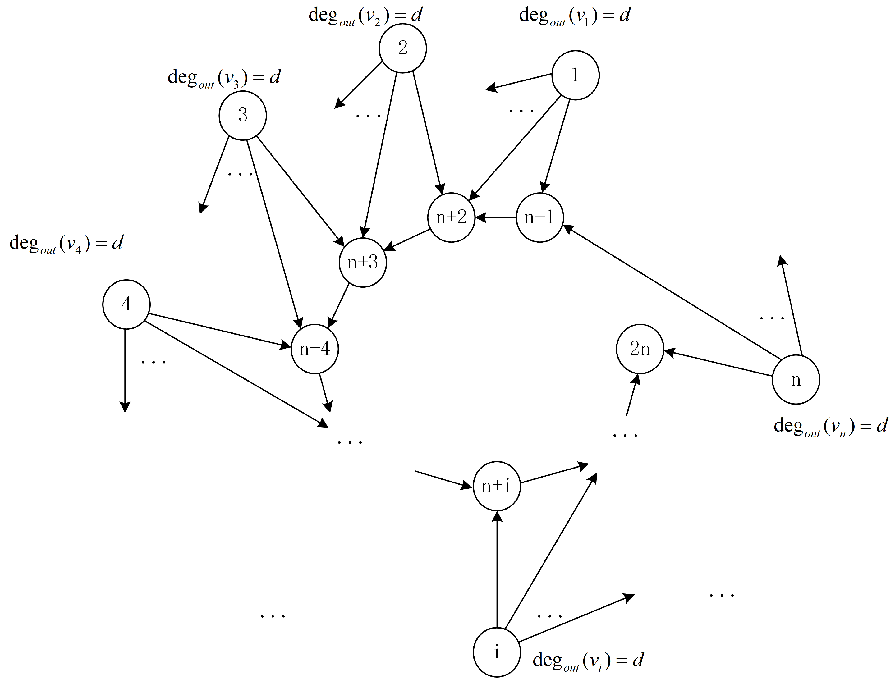
Assumption 4.

Graph $G^{″}$ has a total of n formation leaders numbered as $1,2,\dots ,n$; at the same time, there are n followers numbered as $n+1,n+2,\dots ,2n$. The followers are connected in sequence according to the topological order; a formation leader connects d followers starting from the follower whose number is larger than its own number by n in sequence according to the topological order, which construct a "minimal unit" of a formation leader, where $1\le d\le n,d\in {\mathbb{N}}^{+}$. If a formation leader does not have enough followers to connect in the ordering, then it connects the remaining followers from the $n+1$ follower in the ordering. See Figure 3.

Assumption 5.

Graph $G^{″}$ has a total of n formation leaders numbered as $1,2,\dots ,n$; at the same time, there are n followers numbered as $n+1,n+2,\dots ,2n$. The followers are connected in sequence according to the topological order; a formation leader connects d followers as a "minimal unit", then the n "minimal units" construct the general typology structure of G″. See Figure 4.

Remark 3.

The structure of G″ is constructed by n "minimal units"; the ellipsis in Figure 3 and Figure 4 means there are edges connecting other followers, and d can be any constant less than n and larger than or equal to 2. For example, when $n=4,d=3$, the topology structure is as in Figure 5.

The entire graph G″ is a DAG, and the numbering of the nodes connected to each other follows the topological order. Therefore, the Laplacian matrix of graph G″ is a lower triangular matrix.

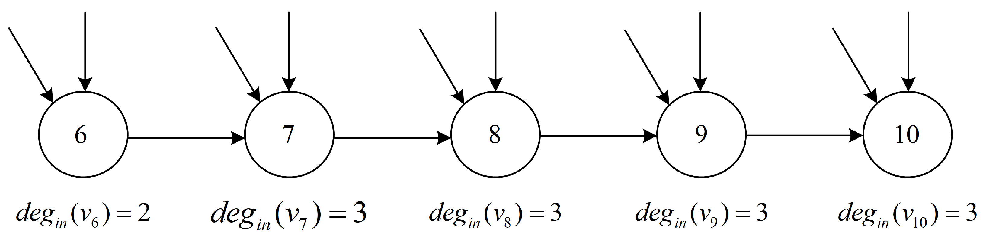
Due to the fact that the addition of a reverse edge is limited to followers only (the formation leader cannot receive signals from followers), according to Lemma 1, in order to study the effect of adding reverse edges on the algebraic connectivity of stem structures, it is necessary to pay attention to the in-degree of the nodes in the stem structure, i.e. nodes numbered from $n+1$ to $2n$ must satisfy the requirements of Lemma 1 for in-degree. By observation, the in-degree of follower node $n+1$ is d, while the in-degree of all other follower nodes is $d+1$. If we choose follower node $n+1$ as the head node and another follower node as the tail node, the in-degree between the follower nodes does not satisfy the condition of Equation (3), i.e., the in-degree of the tail node must not be greater than the in-degree of the head node and all intermediate nodes. Obviously, this case cannot be directly analyzed by Lemma 1.

In order to use Lemma 1 smoothly, a virtual node with an in-degree of 1, denoted as $2n+1$, was added to the original DAG G″. This node can be directly connected to any follower node except for follower node $n+1$ (since node $n+1$ is the first among all follower nodes in the topological order, it cannot serve as the tail node). When a follower node is needed as the tail node, a virtual node with an in-degree of 1 can be added after it, and it can be used as the tail node for the reverse edge analysis. Its specific characteristics are given by Lemma 4.

Lemma 4.

When $1<d\le n$, $d\in {\mathbb{N}}^{+}$, the algebraic connectivity ${\lambda }_{\min }=d$ for the DAG graph G″ under Assumption 4. If a virtual follower node with ${\mathrm{deg}}_{in}\left(v_{2n+1}\right)=1$ is added, connected to any non-follower node other than node $n+1$, the resulting new graph G′ remains a DAG and its Laplacian matrix is a lower triangular matrix. The topology between followers is a stem, as shown in Figure 6. Then, the algebraic connectivity ${\lambda }_{\min }=1$ for the new graph G′.

Proof. 

Due to the Laplacian matrix $L^{″}$ of the original DAG graph $G^{″}$, which is given by $L^{″}=\left[\begin{array}{cc}0& 0\\ {L_2}^{″}& {L_3}^{″}\end{array}\right]\in R^{\left(2n\right)\times \left(2n\right)}$, where

$$L_3^{{}^{″}}=\left[\begin{array}{ccccc}d& & & & \\ {l_{2n,n+1}}^{″}& d+1& & & \\ {l_{n+3,n+1}}^{″}& {l_{n+3,n+2}}^{″}& d+1& & \\ ⋮& ⋮& ⋮& \ddots & \\ {l_{2n,n+1}}^{″}& {l_{2n,n+2}}^{″}& {l_{2n,n+3}}^{″}& \cdots & d+1\end{array}\right]\in R^{n\times n},$$

as $L^{″}$ is a lower triangular matrix, it follows that the diagonal elements are the eigenvalues of $L^{″}$. Its algebraic connectivity is $\Re \left({\lambda }_{\min }\left(L^{″}\right)\right)=d$. After adding a virtual follower to obtain graph $G^{\prime }$, the Laplacian matrix of the new graph $G^{\prime }$ is given by $L^{\prime }=\left[\begin{array}{cc}0& 0\\ {L_2}^{\prime }& {L_3}^{\prime }\end{array}\right]\in R^{(2n+1)\times (2n+1)}$, where ${L_3}^{\prime }=\left[\begin{array}{ccccc}d& & & & \\ {l_{2n,n+1}}^{\prime }& d+1& & & \\ {l_{n+3,n+1}}^{\prime }& {l_{n+3,n+2}}^{\prime }& & & \\ ⋮& ⋮& \ddots & & \\ {l_{2n,n+1}}^{\prime }& {l_{2n,n+2}}^{\prime }& \cdots & d+1& \\ {l_{2n+1,n+1}}^{\prime }& {l_{2n+1,n+2}}^{\prime }& \cdots & {l_{2n+1,2n}}^{\prime }& 1\end{array}\right]\in R^{(n+1)\times (n+1)}$; similarly, $L^{\prime }$ is also a lower triangular matrix, and its diagonal elements are the eigenvalues of $L^{\prime }$. Its algebraic connectivity is $\Re \left({\lambda }_{\min }\left(L^{″}\right)\right)=1$. □

Remark 4.

As stated in item (6) of Lemma 1, if the in-degree of the tail node of a reverse edge is always 1, then the algebraic connectivity will always lie in the range of ${\lambda }_{\min }\in (0,1)$. This makes it easier to compare the effect of adding different reverse edges on the algebraic connectivity in a unified range when considering a stem structure.

Remark 5.

The virtual follower node only receives information from the follower node it is connected to in the graph. Therefore, during the movement process, the trajectory of the virtual follower node coincides completely with that of the follower node it represents. In practical applications, the virtual follower node and the follower node it represents stand for the same unmanned transportation device.

Remark 6.

The virtual node does not actually change the algebraic connectivity or the convergence point of the original graph. The purpose of adding this node is only to facilitate the analysis of changes in the algebraic connectivity of the graph using Lemma 1.

Since the addition of the reverse edge is limited to the followers only, according to clause (1) of Lemma 1, only the eigenvalues corresponding to the nodes within the scope of the reverse edge will change. Therefore, the eigenvalues corresponding to the leader part will not change. In the subsequent analysis of the algebraic connectivity, the formation leader can be ignored, as shown in Figure 7.

In a stem structure with a total of t nodes, there are a total of $\frac{t(t-1)}{2}$ possible reverse edges that can be added. When the tail node is located at the node with the highest index, the number of possible reverse edges that can be added is $t-1$.

For convenience, this article first analyzes the case where the tail node of a reverse edge is located at the highest indexed follower node, and the initial node is one of the remaining follower nodes, the reverse edge that can reduce the algebraic connectivity and minimize the loss of algebraic connectivity is identified. The cases where other followers are the tail node of the reverse edge will be discussed later, and their sizes will be analyzed.

Now, we begin to analyze the case where the tail node of the reverse edge is the follower node with the largest topological order: connect the virtual node $2n+1$ to the follower node with the largest topological order $2n$. According to Lemma 4, we take $2n+1$ as the tail node of the reverse edge, as shown in Figure 8. Since the connection between followers in graph $G^{\prime }$ is a stem structure, adding a reverse edge with the tail node at $2n+1$ and the head node selected from the set of candidate nodes $\Omega =\left\{n+1,n+2,\cdots ,2n\right\}$ must correspond to a reverse range that is a stem structure. The impact of adding a reverse edge on the rate in a DAG with a reverse range that is a stem structure is given by the following proposition.

Proposition 1.

Consider a graph G with $2n+1$ nodes that has a topological order and whose Laplacian matrix is a lower triangular matrix. The graph contains a stem consisting of $n+1$ nodes, each numbered in topological order as $n+1,n+2,\dots ,2n+1$. The node $2n+1$ is a virtual node, and the in-degrees of these nodes have the following characteristics:

• The in-degree of node $n+1$ is a constant d, where $d\ge 1$.
• The in-degree of the virtual node $2n+1$ is a constant 1.
• The in-degree of nodes $n+2,n+3,\dots ,2n$ is a constant $d+1$.
• $d\ge 1$. Now we fix node $2n+1$ as the tail node of the reverse range and select one of the nodes $n+2,n+3,\dots ,2n$ as the head node of the reverse range. Depending on the choice of the head node, we have the following conclusions about the effect of adding a reverse edge on the dominant convergence rate ${\lambda }_{min}$:

(1) 

When selecting $n+2,n+3,\dots ,2n$ as the starting node, the larger the serial number of the selected starting node, the smaller the dominant convergence rate ${\lambda }_{min}$. Among them, selecting node $n+2$ as the starting node results in the maximum algebraic connectivity.

(2) 

When the constant d satisfies $d\ge 2$ and $d\le n$, choosing the node $n+1$ as the head node for the reverse edge will result in a strictly larger algebraic connectivity than choosing $n+2$ as the head node.

Proof. 

(1)

It can be inferred from Lemma 1 that the dominant convergence rate ${\lambda }_{min}\in (d_0,d_1,\dots ,$$d_m,r_1,\dots ,r_m)$ is a function of the first node’s in-degree $d_0$, the in-degrees of the middle nodes $d_i$, and the number of nodes with each in-degree $r_i$. Combining this corollary with the topology shown in Figure 4, when the tail node is fixed and the head node is chosen from nodes $2,3,\dots ,n$, the function ${\lambda }_{min}$ becomes a function of the independent variables $d_0$, $d_1$, and $r_1$, which are as follows: $d_0=d+1$. There is only one type of middle node with in-degree $d_1=d+1$, and the number of middle nodes with in-degree $d_1$ varies depending on the choice of the first node. As the index of the first node selected increases and the value of $r_1$ decreases, while $d_0=d+1$ and $d_1=d+1$ remain unchanged. Since $d\ge 1$ and $d_1\ge 2$, ${\lambda }_{min}(d_0,d_1,r_1)$ strictly increases monotonically with respect to $r_1$. Therefore, the dominant convergence rate decreases as $r_1$ decreases.

(2)

Before adding the reverse edge, as shown in Figure 8, the in-degrees of node $n+1$ and the other nodes in the candidate set $\Omega =\{n+1,n+2,\cdots ,2n\}$ are all different, so we cannot directly compare their convergence rates. In order to compare the convergence rate of selecting node $n+1$ with selecting other head nodes, according to the second statement of Lemma 1, the changed eigenvalues in the reverse scope can be given by the polynomial Equation 4. Applying Equation (4) to the case where node $n+1$ is selected as the head node in Figure 4:

$$(\lambda -1)(\lambda -(d+1)){(d+1-\lambda )}^{(n-1)}=1$$

(14)

Applying Equation (4) to the case where node $n+2$ is selected as the head node in Figure 4:

$$(\lambda -1)(\lambda -(d+2)){(d+1-\lambda )}^{(n-2)}=1$$

(15)

Equations (14) and (15) present the relationship between the dominant convergence rate ${\lambda }_{min}$ and the positive independent variables d and n in the form of implicit functions. To distinguish them, we denote the function $\lambda$ in the implicit function (14) as $y_1$, and the function $\lambda$ in the implicit function (15) as $y_2$, as shown in the following Equations (16) and (17):

$$y_1(d,n):(y_1-1)(y_1-(d+1)){(d+1-y_1)}^{(n-1)}=1$$

(16)

$$y_2(d,n):(y_2-1)(y_2-(d+2)){(d+1-y_2)}^{(n-2)}=1$$

(17)

Dividing both sides of Equations (16) and (17) by each other, we obtain:

$$\frac{(1-y_1){((d+1)-y_1)}^n}{(1-y_2)((d+2)-y_2){((d+1)-y_2)}^{n-2}}=1$$

(18)

Construct a function $F\left(y\right)$ with $y_1$ and $y_2$ as variables:

$$F\left(y\right)=(1-y){(d+1-y)}^n$$

(19)

Transforming Equation (18), we obtain:

$$\begin{array}{c}\hfill \frac{(1-y_1){(d+1-y_1)}^n}{(1-y_2){(d+1-y_2)}^n}·\frac{{(d+1-y_2)}^2}{(d+2-y_2)}=\frac{F\left(y_1\right)}{F\left(y_2\right)}·\frac{{(d+1-y_2)}^2}{(d+2-y_2)}=1\end{array}$$

(20)

Firstly, we study the monotonicity of $F\left(y\right)$ for $y\in (0,1)$.

$$F^{\prime }\left(y\right)=-{(d+1-y)}^n-n(1-y){(d+1-y)}^{n-1}$$

(21)

Since d and n are positive integers, it is obvious that $F^{\prime }\left(y\right)<0$ and $F\left(y\right)$ is decreasing for $y\in (0,1)$.

The second step is to study the relationship between ${(d+1-y_2)}^2$ and $(d+2-y_2)$ in Equation (20). We can take their difference means subtracting one from the other:

$$\begin{array}{c}\hfill h\left(y_2\right)={(d+1-y_2)}^2-(d+2-y_2)={y_2}^2-(2d+1)y_2+(d^2+d-1)\end{array}$$

(22)

We obtain a quadratic function with parameter d. We can find the axis of symmetry $y_2=\frac{(2d+1)}{2}$ and two roots of this function $y_{21}=\frac{(2d+1)-\sqrt{({(2d+1)}^2-4(d^2+d-1))}}{2}$ and $y_{22}=\frac{(2d+1)-\sqrt{({(2d+1)}^2+4(d^2+d-1))}}{2}$. Now we compare the values of $y_1$ and $y_2$ by discussing the possible values of d.

When $d=1$, we can obtain $h\left(y_2\right)=y_2^2-3y_2+1$. When $y_2$ is in the domain of $y_2\in (0,1)$, it can be observed that when $y\in (\frac{3-\sqrt{5}}{2},1)$, $h\left(y_2\right)<0$. In this case, ${(d+1-y_2)}^2<(d+2-y_2)$. By comparing this with Equation (20), we can see that $y_1<y_2$.

When $d\ge 2$, we can obtain the axis of symmetry of the graph of the function $h\left(y_2\right)$ as $y_2=\frac{2d+1}{2}$ and the point of intersection of the function with the $y_2$ axis on the left side as $(\frac{(2d-1)-\sqrt{5}}{2},0)$. Now, when $y_2$ is in the domain of $(0,1)$, the horizontal coordinate of this intersection point is $\frac{(2d-1)-\sqrt{5}}{2}=d+\frac{1-\sqrt{5}}{2}$. Obviously, if $d\ge 2$, then $h\left(y_2\right)>0$ holds for all $y_2\in (0,1)$. By comparing Equation (20), we can see that $y_1>y_2$.

It can be seen that when the positive integer $d\ge 2$ and $d\le n$, the convergence rate of selecting node $n+1$ as the head node is faster than selecting node $n+2$.

□

Considering both the conclusions of Proposition 1 and a comprehensive analysis, it can be concluded that when the positive integer $d\ge 2$ and $d\le n$, selecting the node with the latest topological order as the tail node in the stem structure can reduce the algebraic connectivity of all reverse edges and improve the formation structure. At the same time, selecting the node $n+1$ with the earliest topological order as the starting node for the reverse edge can enable the system to achieve the fastest convergence rate.

Next, we compare the cases of adding reverse edges when other follower nodes in the stem structure, i.e., including nodes $n+2$ to $2n-1$, are selected as the tail node.

Here, we compare the number of nodes crossed by the reverse edges and compare it with the algebraic connectivity obtained from the reverse edges with node $2n$ as the tail node and nodes $n+1$ to $2n-1$ as the starting nodes. The impact of adding a reverse edge on algebraic connectivity is largely determined by the range of nodes crossed by the reverse edge. Since the stem structure is a single-chain structure, the range of nodes crossed can only be a single chain. The specific variables include the in-degree $d_0$ of the starting node, the in-degree $d_i$ of the intermediate nodes, and the number $r_i$ of intermediate nodes with each in-degree. In the model studied in this paper, there is only one type of in-degree for intermediate nodes crossed by the reverse edge, which is $d_1$. When the number of crossed nodes is the same, the number of intermediate nodes with this unique in-degree is also the same. Therefore, the choice of the tail node for the reverse edges does not affect the size of algebraic connectivity, and the difference in algebraic connectivity is only determined by the difference in the in-degree of the starting node,$d_0$.

In the model analyzed in this paper, the difference in the in-degree $d_0$ mainly depends on whether the node $n+1$ with the earliest topological order is selected as the starting node. When node $n+1$ is the starting node, the in-degree of the starting node is $d_0=d$, while for other nodes, the in-degree of the starting node is $d_0=d+1$. Next, we compare the impact of adding reverse edges to algebraic connectivity when the number of crossed nodes is the same for different starting nodes.

When the number of crossed nodes is $t+2$, there are only two possible algebraic connectivity values: when the starting node is the follower node with the smallest index, the in-degree of the starting node is $d_0=d$, and the algebraic connectivity is ${\lambda }_{min}(d,d+1,1)$. For all other nodes as starting nodes, the in-degree of the starting node is $d_0=d+1$, and the algebraic connectivity obtained is ${\lambda }_{min}(d+1,d+1,1)$. To compare the size relationship between these two algebraic connectivity values, the following proposition is given:

Corollary 1.

The conditions are consistent with Proposition 1. When the number of nodes crossed by the reverse edge is the same t, the tail node has an in-degree of 1, and the two algebraic connectivity values with a difference of 1 in the in-degree of the head node, i.e., ${\lambda }_{min}(d+1,d+1,1)$ and ${\lambda }_{min}(d,d+1,1)$, ${\lambda }_{min}(d+1,d+1,1)$ is strictly greater than ${\lambda }_{min}(d,d+1,1)$.

Proof. 

We use point (4) of Lemma 1 and conclude that: for $i=0,1,\dots ,m$, when the other independent variables are fixed, the function ${\lambda }_{min}(d_0,d_1,\dots ,d_m,r_1,\dots ,r_m)$ is strictly monotonically increasing with respect to the independent variable $d_i$. Therefore, when the other independent variables are fixed, ${\lambda }_{min}(d_0,d_1,r_1)$ is strictly monotonically increasing with respect to the in-degree $d_0$ of the first node, so ${\lambda }_{min}(d+1,d+1,1)$ is strictly greater than ${\lambda }_{min}(d,d+1,1)$. □

Combining all the above conclusions, adding a reverse edge on the stem structure of the followers can improve their formation within the convex hull. From the perspective of achieving the maximum convergence rate, selecting a reverse edge in which the first node is the follower node with the smallest index and the last node is the follower node with the largest index can achieve the maximum convergence rate while ensuring improvement in the formation.

Remark 7.

In graph $G^{\prime }$, selecting the reverse edge with the first node as $n+1$ has a faster convergence rate than selecting other follower nodes as the first node. In addition, by increasing d, the algebraic connectivity of graph G can be made closer to the algebraic connectivity of graph $G^{\prime }$, allowing the system to achieve almost the same convergence rate as before adding the reverse edge. However, as the constant d increases, the formation of followers becomes denser. Therefore, d should not be too large.

Corollary 2.

For the follower USV cluster with the communication topology shown in Figure 8, adding such a reverse communication link can improve the formation of the follower fleet while maximizing the dominant convergence rate closest to before adding the reverse edge: the head node of the reverse link is the follower node with the smallest topological order, and the tail node is the follower node with the largest topological order.

Proof. 

This conclusion can be easily proved by the Proofs of Proposition 1 and Corollary 1. □

4. Simulation

First, we obtain the parameters of the USV control protocol based on Algorithm 1 in [16]. While completing the formation containment tracking task, we pay attention to observing the formation of the USV followers. The specific results are as follows:

When $n=5$ and $d=2$, we have the following designed topology, where USV 0 is the tracking leader; USV 1, 2, 3, 4, and 5 are the formation leaders; USV 6, 7, 8, 9, and 10 are the followers; and USV 11 is a fictitious follower. As shown in Figure 9, the connection between the tracking leader and the formation leaders is represented by dashed lines because the analysis of algebraic connectivity does not consider their connection relationship.

Next, based on the given topology, we design the parameters. In the first step, we provide the formation vector $h_L\left(t\right)=[h_1\left(t\right),h_2\left(t\right),h_3\left(t\right),h_4\left(t\right),h_5\left(t\right)]$ for the formation leaders, and plan to maintain a regular pentagon formation centered around the tracking leader, i.e., $h_i\left(t\right)=\left[\begin{array}{c}\cos (t+\frac{2(i-1)\pi }{5})\\ -\sin (t+\frac{2(i-1)\pi }{5})\end{array}\right]$. It can be clearly solved that $v_i\left(t\right)=-\sqrt{2}\sin (t+\frac{(2i-2)\pi }{5}-\frac{\pi }{4})\ne 0$. In the second step, we provide the motion parameters of each USV particle model: $A=\left[\begin{array}{cc}0& 1\\ -2& -1\end{array}\right]$, $B=\left[\begin{array}{c}0\\ 1\end{array}\right]$; it is not difficult to solve for the positive definite matrix $P=\left[\begin{array}{cc}1.5158& 0.2361\\ 0.2361& 0.5723\end{array}\right]$, and it is obvious that the system $(A,B)$ is stable. In the third step, it follows from Lemma 3 in Reference [16] that the positive definite matrix $D_l=diag\{1,1,1,1,1\}$, ${\Phi }_l=\{2,2,2,2,2\}$, $G_f=diag\{0.5041,0.5124,0.5372,0.6116,0.8347,1.5041\}$,

${\Xi }_f=\left[\begin{array}{cccccc}3.02& -0.51& 0& 0& 0& -0.50\\ -0.51& 3.07& -0.54& 0& 0& 0\\ 0& -0.54& 3.22& -0.61& 0& 0\\ 0& 0& -0.61& 3.67& -0.83& 0\\ 0& 0& 0& -0.83& 5.01& -1.50\\ -0.50& 0& 0& 0& -1.50& 3.01\end{array}\right]$. It can be calculated that ${\lambda }_{\max }\left(D_l\right)=1$, ${\lambda }_{\min }\left({\Phi }_l\right)=2$, ${\lambda }_{\min }\left(G_f\right)=0.5$, and ${\lambda }_{\min }\left({\Xi }_f\right)=2$, taking parameters ${\alpha }_1=1\ge 0.5$ and ${\alpha }_2=1\ge 0.25$. From the fourth step, take the parameters $\sigma =0.005$, $\eta =5$, and $\mu =8$. Then, the multi-USV system can accomplish formation containment tracking tasks, and each agent is relatively stationary to each other, maintaining a certain spatial relative position, as shown in Figure 10.

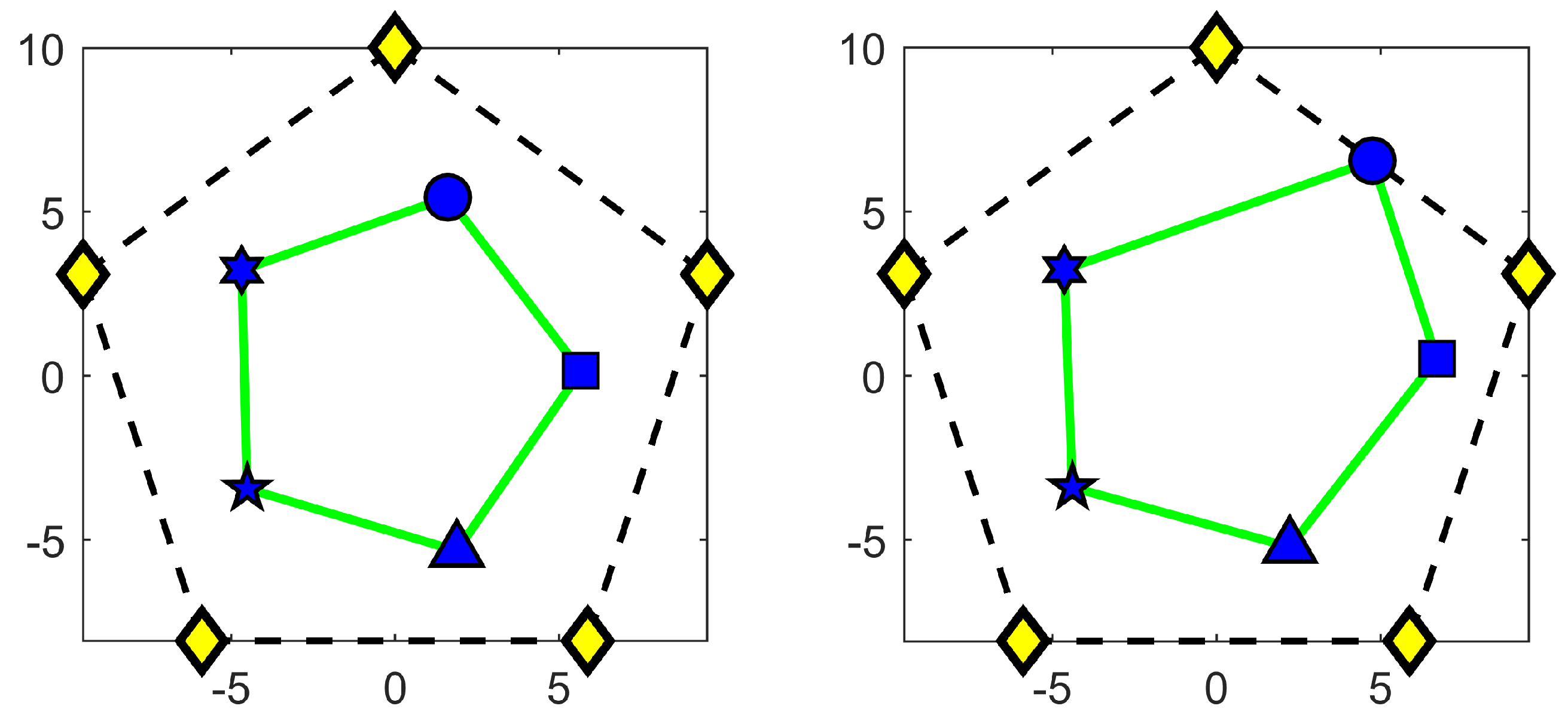
This paper proposes a method of adding a reverse edge to optimize the convergence position of followers in the formation. To demonstrate the effectiveness of this method, we use the preset formation with an added reverse edge shown on the left side of Figure 11 as a comparative experiment. The preset formation is presented as a pentagon similar to the leader’s formation, and it should be noted that, according to Remark 6, the convergence positions of the virtual node 11 and follower node 10 always remain consistent. Based on this, we remove the virtual node 11, connect follower 10 directly to follower 6, and add a reverse edge to adjust the convergence positions of other followers. By doing so and comparing it with the formation of followers on the right side of Figure 11 without the addition of reverse edges, we can obtain the following advantages:

(1)

The distance between each USV is relatively far, which can reduce the possibility of collision between them.

(2)

After adding reverse edges, the convergence positions of the followers are more evenly distributed and maintain a fixed angular difference with the formation leader, which has better obstacle avoidance ability in complex sea areas. In contrast, in the case where reverse edges are not added (on the right side of Figure 11), there are two followers, 6 and 10, who are very close to the formation leader and even appear on the edge of the convex hull. This obviously does not benefit the safety and stability of the formation.

As can be seen, the communication topology designed in this article exhibits rotational symmetry in the relationship between the convergence positions of followers with the addition of reverse edges and the position of the formation leader. Thus, the formation of the followers is similar to that of the formation leader. If the formation of the leader is in the shape of a regular polygon, the followers can converge into a similar polygon shape inside the convex hull uniformly.

Next, we ignore the tracking leader and compare the effects of adding different reverse edges to the stem structure of the original follower network on the algebraic connectivity that characterizes the convergence rate.

This article proposes a method of adding a reverse edge to optimize the formation of the team. As shown in Figure 12, in the follower network, we choose any two nodes on the stem and take the node with a smaller index as the head node while artificially setting a node with an in-degree of 1 as the tail node of the reverse edge after the node with a larger index. This approach results in an algebraic connectivity of ${\lambda }_{\min }\left(G\right)=1$. When we add reverse edges, the algebraic connectivity decreases. Figure 13 shows the effects of different reverse edges on the algebraic connectivity.

Considering the follower network part of the communication topology, as shown in Figure 12, the network structure appears as a stem. We choose any two points on the stem, and according to the topological order, the node with a smaller index is taken as the head node. For ease of analysis, a virtual node with an in-degree of 1 is artificially added as the tail node of the reverse edge after the node with a larger index, in accordance with the requirements of Proposition 1. This makes the algebraic connectivity ${\lambda }_{\min }\left(G\right)=1$. When the reverse edge is added, the algebraic connectivity decreases. The change in the algebraic connectivity with the addition of different reverse edges is shown in Figure 13.

In Figure 13, the vertical axis represents the algebraic connectivity of the communication topology, and the horizontal axis represents the first node number of the reverse edge where $t1,t2,t3$, and $t4$, respectively, represent a node with an in-degree of 1 that is virtually added as the tail node of the reverse edge after nodes 10, 9, 8, and 7.

By observing Figure 13 and only looking at the images where the first node of the reverse edge is 7, 8, or 9, the algebraic connectivity after adding the reverse edge can be expressed as the function ${\lambda }_{\min }(3,d,r)$, where d is a positive constant representing the unique in-degree of the middle node in the reverse edge, and r represents the number of nodes in the middle node with an in-degree of d. We can verify some conclusions:

(1)

It can be seen that when $d>1$, the larger the value of r, the smaller the algebraic connectivity ${\lambda }_{\min }$.

(2)

The impact of the reverse edge on the algebraic connectivity ${\lambda }_{\min }$ is only related to the range covered by the reverse edge and the in-degree of the nodes within that range, and is independent of the location of the reverse edge.

Remark 8.

The fact that the location of the reverse edge does not affect the algebraic connectivity can be illustrated by the following example: for instance, when the virtual node after 8 is connected to 7, the virtual node after 9 is connected to 8, and the virtual node after 10 is connected to 9, even though the first and last nodes are not the same; their algebraic connectivity is the same because the length covered by the reverse edge and the in-degree of the nodes it covers are the same.

The following experiments compare the convergence rates when the tail node of the reverse edge is fixed and the first node is either the node with the earliest topological order or the follower node with the second earliest topological order. 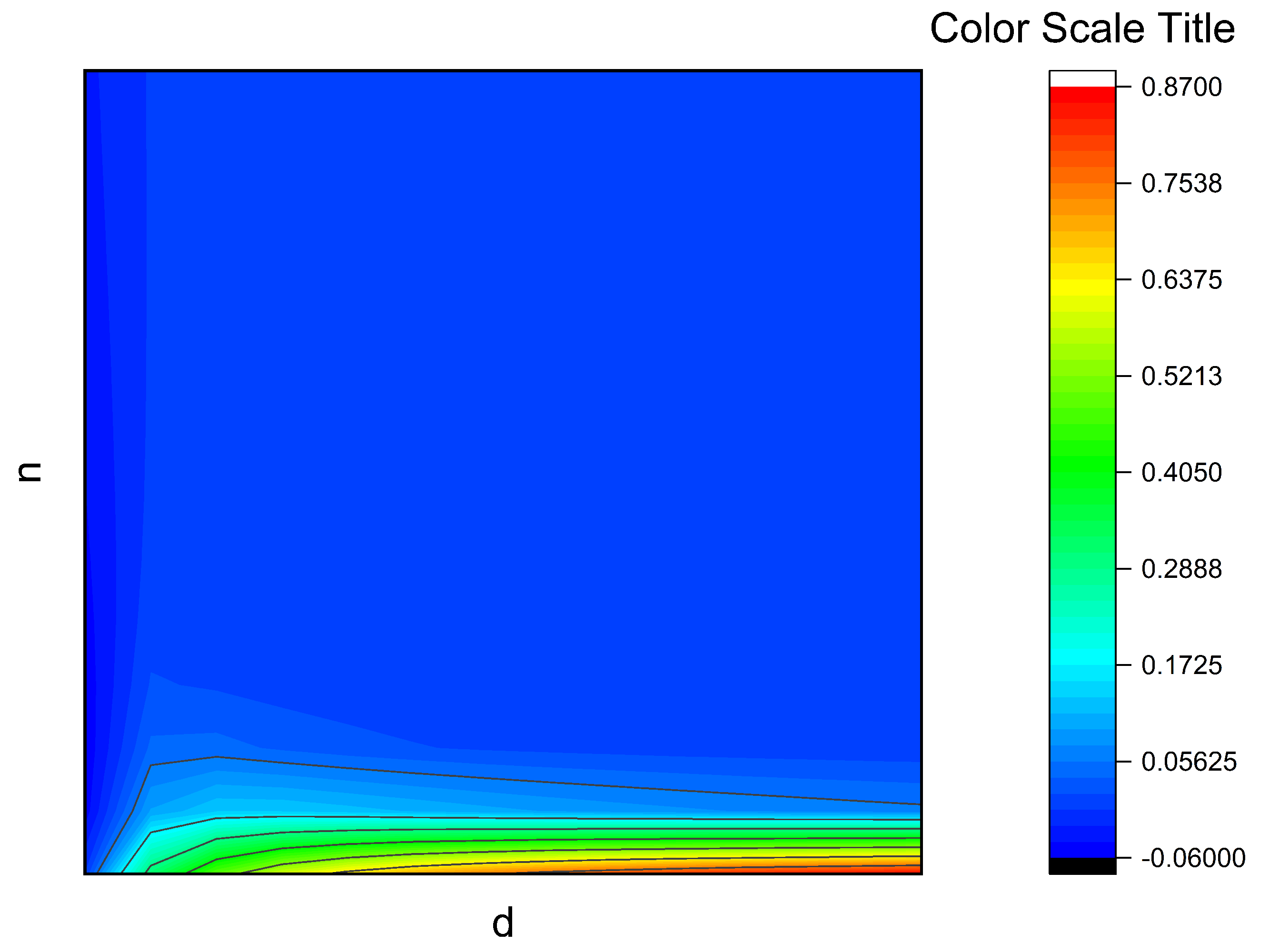Comparing the algebraic connectivity function values for the two cases is not straightforward because ${\lambda }_{\min }(d_0,d,r)$ for both cases has a constant in-degree d for the middle node, but different independent variables, namely the in-degree of the first node $d_0$ and the number of middle nodes with in-degree d: r(which is the number of middle nodes in this structure), making direct comparison difficult.To investigate this problem more generally, we consider the difference between the algebraic connectivity of the follower node with the smallest sequence number and the follower node with the second smallest sequence number, when the unique in-degree d of the middle node in the reverse edge is in the range $(1,14)$ and the number of middle nodes r is in the range $(1,14)$. As shown in Figure 14, when d is close to 1, the difference between the two is negative. However, when $d>1$, the difference is greater than zero, and as d or r increases, the difference between the two algebraic connectivity values approaches zero, but always remains strictly greater than zero.

Therefore, it can be verified that when $d>1$, adding a fixed tail node reverse edge and selecting the reverse edge of the minimum topological order node as the first node will lead to a strictly higher dominant convergence rate than selecting the reverse edge of the second smallest topological order node as the first node.

The result in Proposition 1 can therefore be easily verified.

5. Conclusions

The formation problem of followers in multi-USV formation tracking has been investigated in this article, and a method of adding a reverse link to a specific communication network structure has been proposed to improve the formation of followers while minimizing the loss of dominant convergence rate. To analyze the impact of adding a reverse edge on the algebraic connectivity of a class of stem-based network structures, a method of adding a virtual node has been introduced in this paper and the impact of adding reverse edges on the algebraic connectivity of a follower USV communication topology based on a stem has been analyzed. Based on this analysis, a method of adding only one reverse edge has been proposed to improve the algebraic connectivity of the communication topology and make the follower USV formation scattered, which is beneficial for collision avoidance among USVs. At the same time, the original DAG’s dominant convergence rate has been preserved as much as possible. Compared with general topology reconstruction methods, the advantage of this method is that it only adds one reverse edge to the original DAG. Simulation experiments have been conducted to compare the formation shapes of USV followers before and after adding a reverse edge, and to verify the improvement in the follower formation by adding reverse edges. The impact of adding different reverse edges on algebraic connectivity has also been compared through simulation experiments, and the proposed method has been shown to have the smallest convergence rate loss.