Novel Algorithm for Linearly Constrained Derivative Free Global Optimization of Lipschitz Functions

Abstract

This paper introduces an innovative extension of the DIRECT algorithm specifically designed to solve global optimization problems that involve Lipschitz continuous functions subject to linear constraints. Our approach builds upon recent advancements in DIRECT-type algorithms, incorporating novel techniques for partitioning and selecting potential optimal hyper-rectangles. A key contribution lies in applying a new mapping technique to eliminate the infeasible region efficiently. This allows calculations to be performed only within the feasible region defined by linear constraints. We perform extensive tests using a diverse set of benchmark problems to evaluate the effectiveness and performance of the proposed algorithm compared to existing DIRECT solvers. Statistical analyses using Friedman and Wilcoxon tests demonstrate the superiority of a new algorithm in solving such problems.

1. Introduction

Global optimization is an active and important research area that focuses on discovering the best global solution for an objective function within a given domain. To tackle this challenging problem, numerous cutting-edge solution techniques have been devised. Among these, line search methods have gained widespread usage [1], involving iterative searches for the optimum by following a predetermined search direction. These methods have demonstrated their effectiveness in various domains of problems [2,3]. Another category of techniques comprises meta-heuristic algorithms, which draw inspiration from natural phenomena and problem-solving heuristics. Examples of such algorithms include genetic [4], particle swarm [5], and simulated annealing [6], which have achieved significant popularity and adoption. However, there have been developments in the form of more efficient methods and extensions [7,8,9]. Furthermore, advanced optimization methods such as Bayesian optimization [10] and the radial basis function [11] employ surrogate models to approximate the objective function, enabling an efficient guide of the search process. These techniques play a vital role in addressing complex and computationally demanding optimization problems.

This paper focus on a Lipschitz global optimization [12,13] problem presented in the following form:

$$\begin{array}{cccc}\hfill & \underset{\mathbf{x}\in D}{min}\hfill & \hfill & f\left(\mathbf{x}\right),\hfill \\ \hfill & \mathbf{A}\mathbf{x}\le \mathbf{b},\hfill \end{array}$$

(1)

where $\mathbf{A}\in {\mathbb{R}}^{m\times n},\mathbf{b}\in {\mathbb{R}}^m$ and $D=[\mathbf{l},\mathbf{u}]=\{\mathbf{x}\in {\mathbb{R}}^n:l_j\le x_j\le u_j,j=1,\dots ,n\}$. Here, D represents a full-dimensional convex polytope in which the minimization of the objective function $f:{\mathbb{R}}^n\to \mathbb{R}$ takes place. The feasible region consists of points that satisfy all constraints and is denoted

$$D^{\mathrm{feas}}=D\cap \mathsf{\Omega },\mathrm{where}\mathsf{\Omega }=\{\mathbf{x}\in {\mathbb{R}}^n:\mathbf{A}\mathbf{x}\le \mathbf{b}\}.$$

(2)

For convergence, we assume that the objective function $f\left(\mathbf{x}\right)$ is Lipschitz continuous, at least in the vicinity of the globally optimal solution. However, the function can be non-linear, non-differentiable, non-convex, and multi-modal. Consequently, traditional optimization methods that rely on derivative information do not apply to such problems.

Global optimization of a non-linear objective function subject to linear constraints is a significant topic in mathematical programming, as it covers numerous real-world optimization problems. For example, in engineering design, the optimal design of structures, circuits, and manufacturing processes often involves linear constraints [14]. Similarly, portfolio optimization problems commonly involve linear constraints, such as budget restrictions or constraints on asset allocation percentages [15]. Furthermore, the optimal design and operation of chemical processes are subject to linear constraints arising from considerations such as material balances, equipment capacities, and safety constraints [16]. These examples highlight the diverse domains where linearly constrained non-convex global optimization problems arise.

The algorithm DIRECT [17] is widely recognized for its effectiveness in global optimization, particularly for box-constrained problems. It utilizes a deterministic sampling strategy that enables the discovery of global optima without derivative information. This makes it suitable for handling complex, multi-modal, and non-differentiable objective functions. Since the algorithm was first published, researchers have worked to improve its performance by introducing new and more efficient sequential and parallel variants [18,19,20,21,22,23,24,25,26,27,28]. Comprehensive numerical benchmark studies [29,30,31] demonstrated a very promising performance of DIRECT-type algorithms compared to other derivative-free global optimization methods.

The DIRECT-type algorithms have also shown their effectiveness in solving a wide range of problems with different types of constraints, including those described in Equation (1). Several studies, such as [18,24,32,33,34,35,36], have proposed DIRECT-type algorithms to handle general constraints and “hidden” constraints [37,38,39]. Most of these methods are based on penalties and auxiliary functions. These functions penalize violations of the constraints, ensuring that solutions adhere to the constraints. However, one of the main challenges with penalty-based approaches is the need to adjust the parameters, as the performance of these methods is highly sensitive to the chosen parameters [24,40]. To address this issue, researchers have explored techniques such as automatic penalty setting modification during optimization [18,24,34,35,36]. This leads to more reliable results than methods with manually selected penalty parameters. However, these methods primarily deal with bound constraints and face challenges when encountering infeasible regions. This becomes particularly difficult for DIRECT-type algorithms, as they need to subdivide these regions to uncover feasible regions, resulting in a significant number of wasted function evaluations. To address this issue, only two DIRECT-type algorithms have been specifically designed for problems with linear constraints. In [40], the authors proposed two simplicial partitioning approaches to handle linearly constrained problems, using simplices to cover the feasible region. However, these simplicial partitioning methods are mainly limited to lower-dimensional problems.

This paper presents a new algorithm of type DIRECT designed specifically to address the global optimization problems stated in Equation (1). Building on recent advances in DIRECT-type algorithms, we have integrated novel techniques for partitioning and selecting potential optimal hyper-rectangles. A notable innovation in our approach is the adoption of mapping techniques that efficiently eliminate the infeasible region, allowing computations exclusively within the region delimited by the linear constraints. Through extensive testing using the latest and substantially expanded version of the DIRECTGOLib v1.3 benchmark library [41], this study comprehensively investigates the performance and effectiveness of our proposed algorithm. Furthermore, to ensure the reliability and significance of our results, we employ statistical analyses, including the Friedman [42] and Wilcoxon [43] tests, to validate the superiority of our algorithm over existing DIRECT solvers for such problems.

Paper Contributions and Structure

The contributions of the paper can be summarized as follows:

• The review of techniques proposed to tackle linearly constrained problems within the framework of DIRECT-type algorithms.
• Introduction of a novel and distinctive DIRECT-type algorithm explicitly designed for non-convex problems involving linear constraints.
• The substantial enhancement of the DIRECTGOLib v1.3 benchmark library by incorporating 34 lineary-constrained test problems.
• The provision of the novel algorithm developed as an open-source resource to ensure the full reproducibility and reusability of all results.

The remaining sections of this paper are structured as follows. In Section 2.1, we provide a review of the original DIRECT algorithm, while Section 2.2 covers its relevant modifications for problems with constraints. Section 3 introduces a novel algorithm based on the DIRECT approach. In Section 4, we provide and discuss the results of our numerical investigation using a set of 67 test problems from the DIRECTGOLib v1.3 library. Finally, in Section 5, we conclude the paper and outline potential directions for future research.

2. Materials and Methods

This section provides an overview of the classical DIRECT algorithm and its extensions to handle constraints.

2.1. The Original DIRECT Algorithm for Box-Constrained Global Optimization

We begin by briefly introducing the original DIRECT algorithm [17], which is a recognized approach for box-constrained global optimization. This algorithm effectively explores the search space by partitioning it into hyper-rectangles and iteratively refining the search through function evaluations. Notably, the DIRECT algorithm is specifically designed to handle box-constrained optimization problems of the form:

$$\underset{\mathbf{x}\in D}{min}f\left(\mathbf{x}\right).$$

(3)

In the initial stages, the DIRECT algorithm normalizes the original domain $D=[\mathbf{l},\mathbf{u}]$ into a unit hyper-rectangle $\overline{D}=[\overline{\mathbf{l}},\overline{\mathbf{u}}]=[\mathbf{0},\mathbf{1}]=\{\overline{\mathbf{x}}\in {\mathbb{R}}^n:0\le {\overline{l}}_j\le {\overline{x}}_j\le {\overline{u}}_j\le 1,j=1,\dots ,n\}$. The algorithm refers only to the original space $\left(D\right)$ that evaluates the objective function.

The search process in the DIRECT algorithm begins with an initial evaluation of the objective function at the midpoint ${\overline{\mathbf{x}}}^1=\left(\frac{1}{2},\dots ,\frac{1}{2}\right)$ of the first unit hyper-rectangle $\overline{D}={\overline{D}}_0^1$. This evaluation serves as the starting point for the algorithm’s search space exploration. The goal is to identify and select hyper-rectangles that are most promising.

Initially, there is only one hyper-rectangle available. Therefore, the selection process is straightforward. The DIRECT algorithm employs an n-dimensional trisection approach, dividing each selected hyper-rectangle into three equal sub-rectangles along each dimension. The objective function is evaluated only once for each newly created hyper-rectangle.

The selection process plays a crucial role in each subsequent iteration $\left(k\right)$ of the algorithm. The objective is to identify the most promising candidates for further investigation, allowing the DIRECT algorithm to effectively navigate the search space and prioritize the exploration of regions with the greatest promise of finding global optima. The formal requirement of potentially optimal hyper-rectangles (POH) in future iterations is stated in Definition 1.

Definition 1. 

Let denote the sampling point as ${\mathbf{x}}^i$ and the measure of the hyper-rectangle $\left({\overline{D}}_k^i\right)$ as ${\overline{\delta }}_k^i$. Let $\epsilon >0$ be a positive constant, and let $f^{min}$ be the best value currently found for the objective function. A hyper-rectangle ${\overline{D}}_k^h$, where $h\in {\mathbb{I}}_k$ (the index set identifying the current partition), is considered potentially optimal if there exists a positive constant $\tilde{L}$ (also known as the rate-of-change or Lipschitz constant) such that

$$\begin{array}{ccc}\hfill f\left({\mathbf{x}}^h\right)-\tilde{L}{\overline{\delta }}_k^h& \le & f\left({\mathbf{x}}^i\right)-\tilde{L}{\delta }_k^i,\forall i\in {\mathbb{I}}_k,\hfill \end{array}$$

(4)

$$\begin{array}{ccc}\hfill f\left({\mathbf{x}}^h\right)-\tilde{L}{\overline{\delta }}_k^h& \le & f^{min}-\epsilon \left|f^{min}\right|,\hfill \end{array}$$

(5)

where the measure of the hyper-rectangle ${\overline{D}}_k^i$ is

$${\overline{\delta }}_k^i=\frac{1}{2}\parallel {\overline{\mathbf{u}}}^i-{\overline{\mathbf{l}}}^i\parallel .$$

(6)

In Equation (6), the $\parallel .\parallel$ on the right-hand side represents the standard Euclidean 2-norm. It is worth mentioning that certain studies [44,45] have examined alternative non-Euclidean norms in their research investigations. A hyper-rectangle ${\overline{D}}_k^h$ is considered potentially optimal if it meets two requirements. First, the lower Lipschitz bound for the objective function, calculated using the left-hand side of (4), should be the smallest among all hyper-rectangles in the current partition, with some positive constant $\tilde{L}$. The second requirement is that the lower bound of the hyper-rectangle must be better than the current best solution $\left(f^{\min }\right)$. Specifically, it should be less than or equal to $f^{\min }-\epsilon \left|f^{\min }\right|$. This condition serves as a threshold to prevent the DIRECT algorithm from wasting function evaluations on extremely small hyper-rectangles that are unlikely to lead to significant improvements. The value of $\epsilon$ used in practice can vary, and in work [17], good results were achieved with values of $\epsilon$ ranging from ${10}^{-3}$ to ${10}^{-7}$. Once all the selected potentially optimal hyper-rectangles have been sampled and subdivided, the iterative process continues until some stopping criterion is met. Common stopping conditions employed in the DIRECT algorithm encompass reaching the maximum limit of objective function evaluations, iterations, execution time, or attaining a specific target value for the objective function.

2.2. Extensions of the DIRECT Algorithm for Problems with Constraints

Although the classical DIRECT algorithm is effective for box-constrained optimization problems, it requires modifications to handle optimization problems with constraints. We discuss the existing approaches and adaptations that have been proposed to extend the capabilities of the DIRECT algorithm for constrained optimization problems.

2.2.1. Approaches Based on Simplicial Partitioning

In our previous work [40], we extended the original DISIMPL algorithm, which is based on simplicial partitioning, to handle problems with linear constraints [46,47]. Simplicial partitioning is particularly suitable for addressing problems with linear constraints because simplices can effectively cover the search space defined by these constraints. This approach allows the simplicial partitioning algorithms (Lc-DISIMPLc and Lc-DISIMPLv) [40] to perform the search exclusively within the feasible region, distinguishing it from other approaches of the type DIRECT. However, it should be noted that calculating the feasible region requires solving $2n+m$ linear n-dimensional systems, as demonstrated by the authors in [40]. This operation exhibits exponential complexity, which limits the effectiveness of the proposed algorithm for problems with relatively small values of n and m.

2.2.2. Penalty and Auxiliary Function Approaches

The first approach to handling constrained problems was introduced in [18] and implemented as glcSolve in TOMLAB software [21]. This approach employs an auxiliary function that penalizes any deviation of the function value from the global minimum value $\left(f^{*}\right)$. The penalty function does not impose any penalty on function values below $f^{*}$; it only applies when violating the constraints. Moreover, a weighted sum of constraint violations is assigned to each value of the function. The penalty function achieves its minimum value of zero solely at the global minimum, while at any other point, it assumes positive values indicating sub-optimality or infeasibility. Additionally, the glcSolve algorithm removes hyper-rectangles where it can be demonstrated that the linear constraints cannot be satisfied.

Several years later, an alternative approach [33] based on DIRECT was introduced that utilizes an exact L1 penalty. Experimental results demonstrated promising results with this approach. However, a major drawback is the manual setting of the penalty parameters for each constraint function by the user. In practice, the selection of penalty parameters is a crucial task that can have a significant impact on the algorithm’s performance [24,34,40,47,48].

Two other approaches based on penalty functions were introduced in [35,36]. These algorithms feature an automatic update rule for the penalty parameter, and under certain weak assumptions, the penalty parameters are updated a finite number of times.

In [24], a novel extension of the DIRECT algorithm called DIRECT-GLce was introduced. This algorithm employs an auxiliary function approach that combines objective and constraint functions. The DIRECT-GLce algorithm operates in two distinct phases: one focuses on locating feasible points, while the second aims to improve the current feasible solution. During the initial phase, DIRECT-GLce samples the search space and minimizes the sum of constraint violations. Once feasible points are identified, the algorithm improves these feasible solutions. The proposed algorithm operates without penalty parameters and ensures convergence to a feasible solution.

2.2.3. Filtering Approach

Another recent DIRECT-type approach [32] also aims to simultaneously minimize constraint violations and objective function values. The suggested algorithm employs filter methodology [49] and divides the main set into three subsets. The filtering strategy prioritizes selecting potentially optimal candidates as follows: first, hyper-rectangles with feasible center points are chosen, followed by those with infeasible but non-dominated center points, and finally, those with infeasible and dominated center points.

2.2.4. Alternative Approaches without Utilizing Constraint Information

The first and most straightforward extension of the DIRECT algorithm to handle the constrained optimization problem is based on the barrier approach, as described in [37]. In this approach, infeasible points are assigned a very high value, ensuring that no infeasible hyper-rectangles are subdivided as long as there are feasible hyper-rectangles of the same size with a feasible midpoint. The strategy was extended in [38], where the authors suggested incorporating a subdividing step. After subdividing all traditional POHs, a new subdividing step is initiated, where all hyper-rectangles with infeasible midpoints are also subdivided. The authors demonstrated that this extra step effectively decomposes the boundaries of the hidden constraints and efficiently exposes the edges of the feasible region.

Another extension of the DIRECT algorithm is based on the neighborhood assignment strategy and was also proposed in [37]. In this approach, the value assigned to an infeasible point is based on the objective function values found in neighboring feasible points.

In the most recent proposals [39], the authors suggested a different approach to handling constraints. The proposed method assigns a value to an infeasible hyper-rectangle, depending on the distance of its center to the current best minimum point. This way, infeasible hyper-rectangles close to the current minimum point are not penalized with large values. This approach allows for a faster and more comprehensive examination near the feasible region boundary.

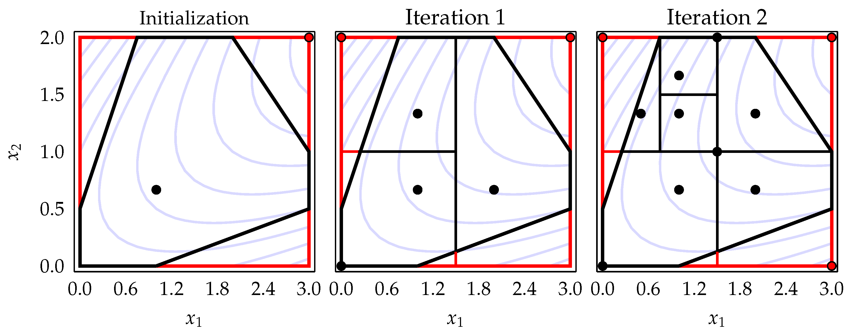
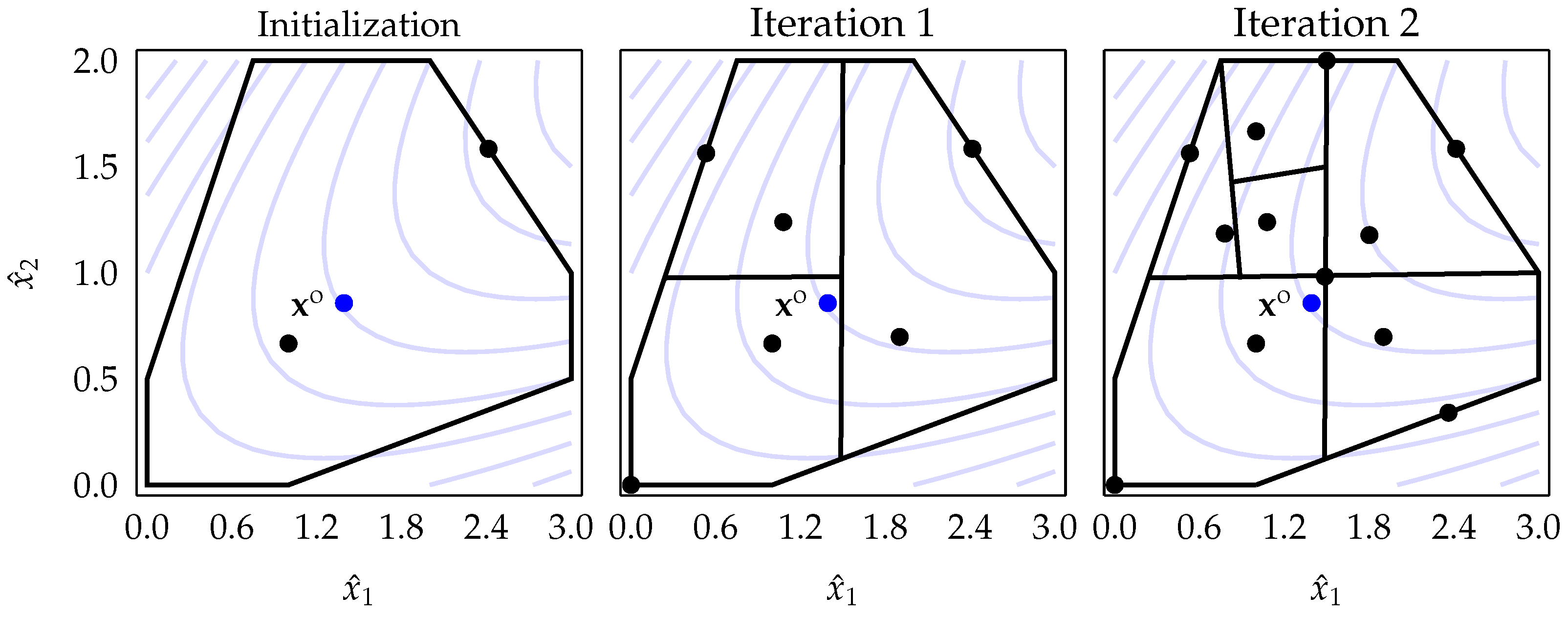
3. Description of the Proposed mBIRECTv-GL Algorithm

This section introduces our novel algorithm based on the DIRECT-type framework and incorporates mapping methods to handle linear constraints efficiently.

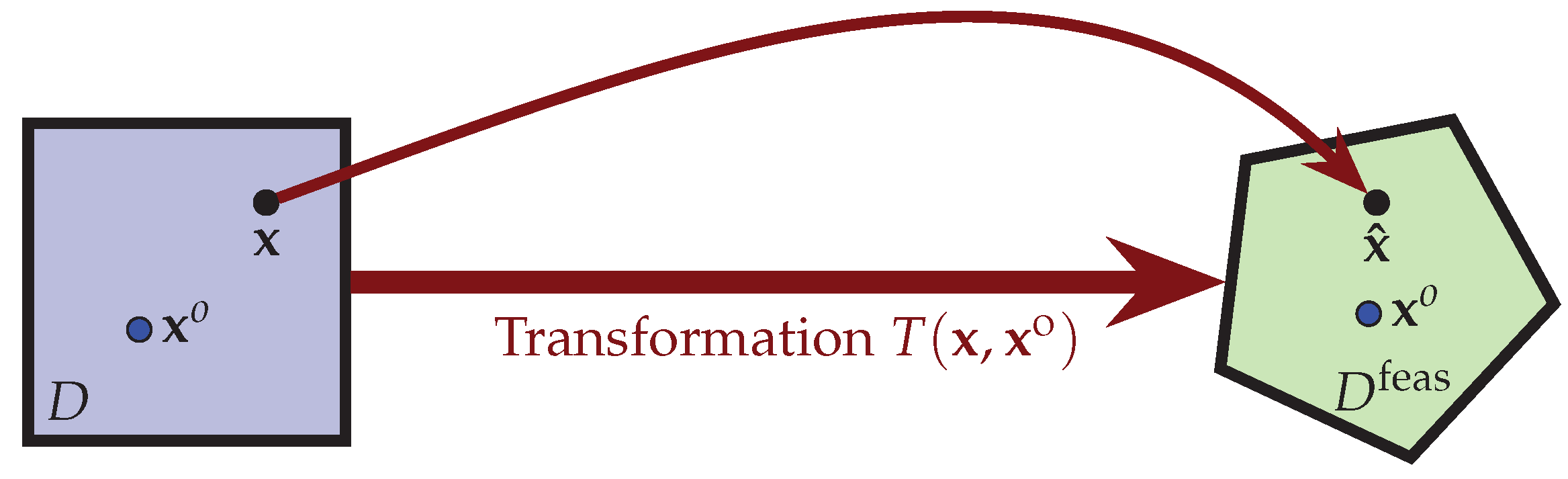
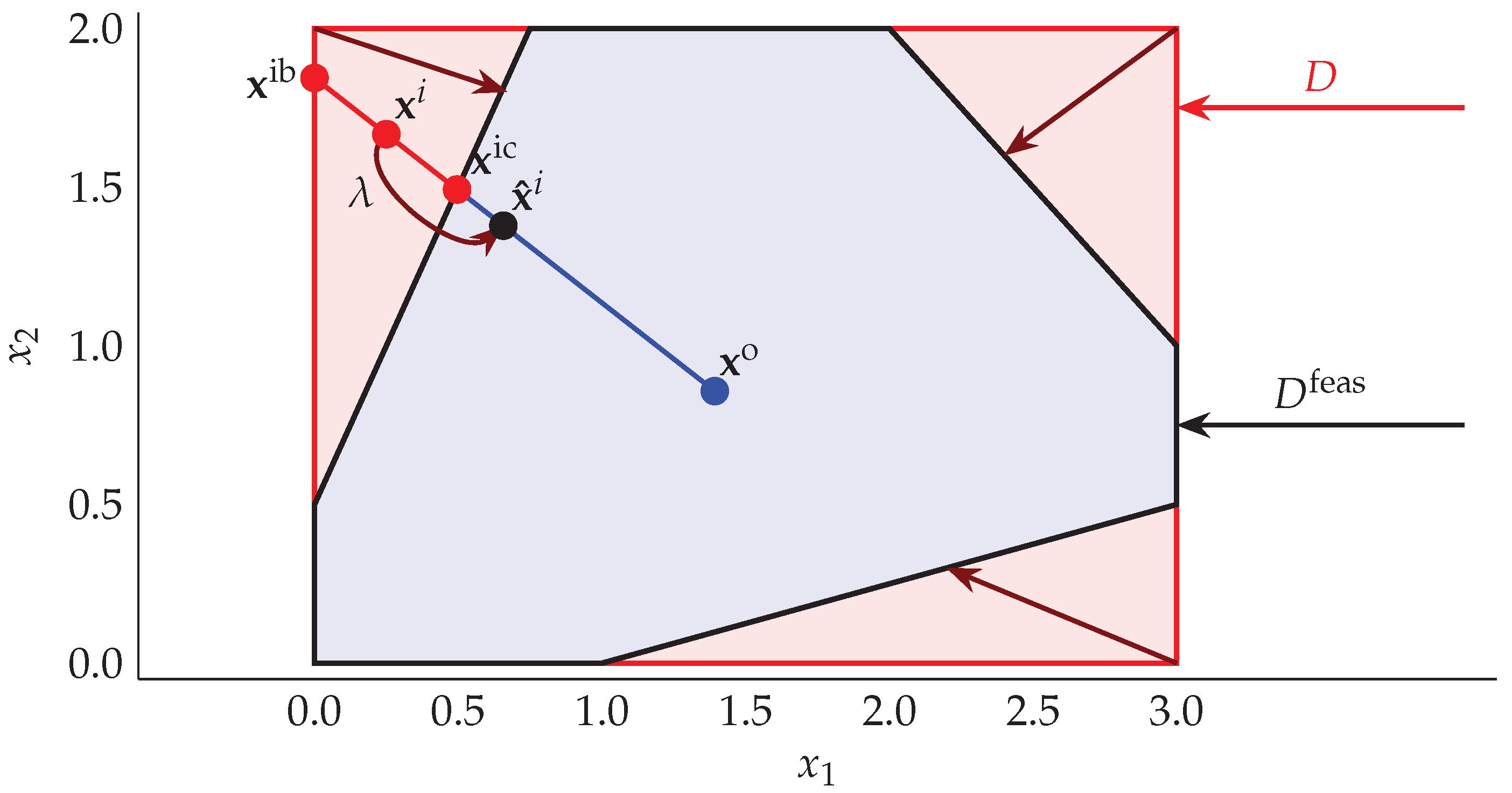
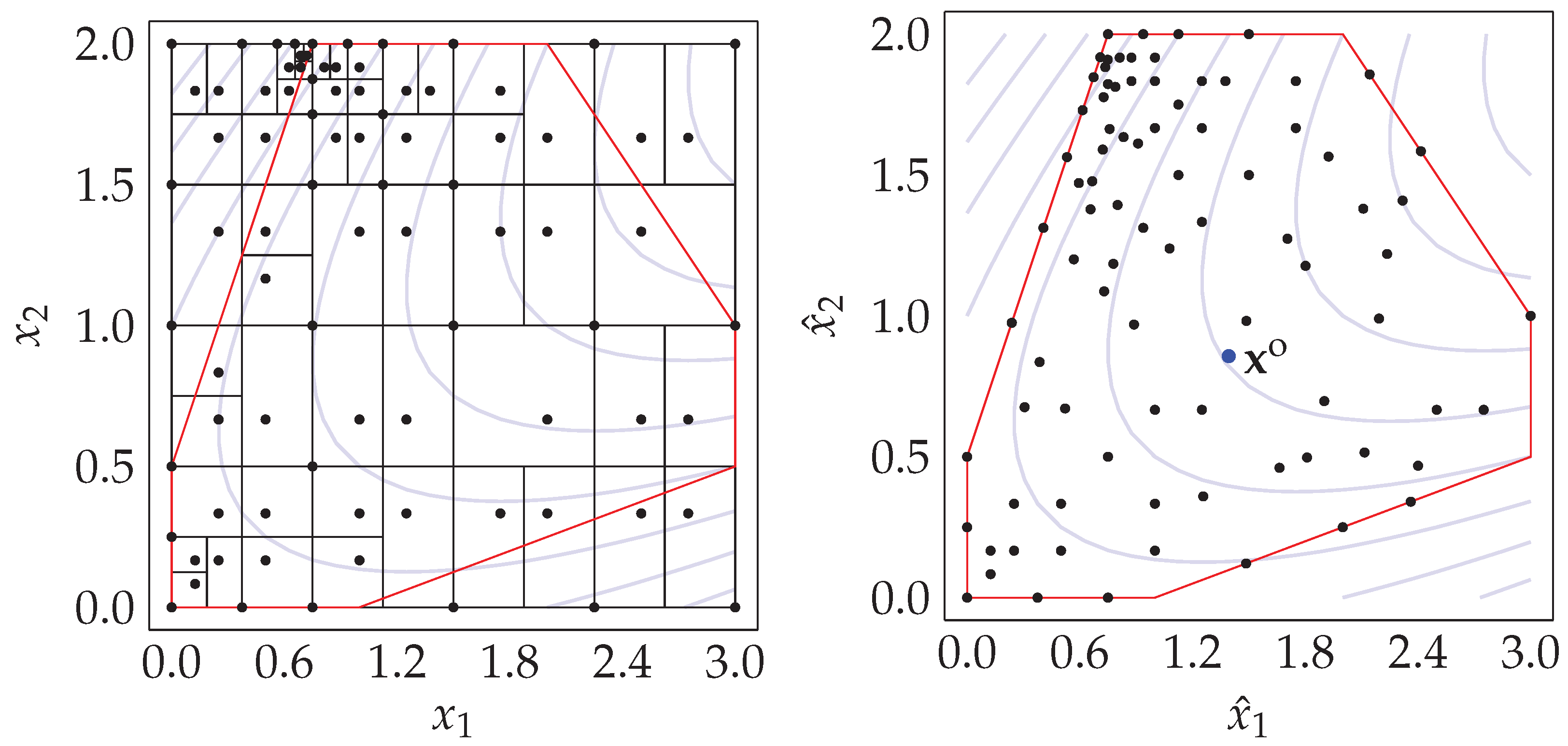
3.1. Efficient Bijective Mapping: Construction and Methodological Details

We describe our technique to map a hyper-rectangle onto a linearly constrained polytope. By employing this transformation (mapping), we aim to leverage the benefits of the DIRECT algorithm to address linearly constrained global optimization problems. The mapping allows us to work within a hyper-rectangular domain D, facilitating the application of the DIRECT algorithm’s efficient search strategies.

The linear constraints imposed in the problem formulation define a region in the original coordinate system that might not align with the DIRECT algorithm, which operates on hyper-rectangles. To bridge this gap, we introduce a transformation that maps the hyper-rectangle onto a linearly constrained region, as illustrated in Figure 1.

Using this approach, we avoid directly solving linearly constrained problems and instead utilize one-to-one mapping. This mapping transforms the points from the hyper-rectangular domain, D, to the feasible space, $D^{\mathrm{feas}}$. Therefore, the solution to the problem:

$$\underset{\mathbf{x}\in D}{min}f\left(T(\mathbf{x},{\mathbf{x}}^o)\right),$$

(7)

yields the solution to the original problem. Here, ${\mathbf{x}}^o$ represents the interior reference point, which coincides in both sets and plays an important role in the mapping. It is essential for the point ${\mathbf{x}}^o$ to be strictly feasible:

$$\mathbf{A}{\mathbf{x}}^o<\mathbf{b}.$$

(8)

Various methods can be used to find ${\mathbf{x}}^o$ as described in [24,34,39,50]. We employ an adapted variation of the technique introduced in [51] that builds on the approach described in [50]. This method finds a set of vertices defined by linear constraints and uses them to calculate the midpoint of $D^{\mathrm{feas}}$.

Let us formalize the mapping process using the Horst1 test problem as an example (see Figure 2). The mapping $T({\mathbf{x}}^i,{\mathbf{x}}^o)$ transforms any point ${\mathbf{x}}^i\in D$ to ${\widehat{\mathbf{x}}}^i\in D^{\mathrm{feas}}$:

$${\widehat{\mathbf{x}}}^i={\mathbf{x}}^i+{\lambda }^i({\mathbf{x}}^o-{\mathbf{x}}^i).$$

(9)

The parameter ${\lambda }^i$ is calculated as:

$${\lambda }^i=\frac{\left|\right|{\mathbf{x}}^{ic}-{\mathbf{x}}^{ib}\left|\right|}{\left|\right|{\mathbf{x}}^o-{\mathbf{x}}^{ib}\left|\right|},$$

(10)

where ${\mathbf{x}}^{ic}$ represents the intersection point of the closest linear constraint (to ${\mathbf{x}}^{ic}$) and the line passing through points ${\mathbf{x}}^o$ and ${\mathbf{x}}^i$. Similarly, ${\mathbf{x}}^{ib}$ is the intersection point of the closest boundary constraint and the same line. The ratio $\lambda \in [0,1)$ is a relative multiplier used to move points in the direction of a vector $({\mathbf{x}}^o-{\mathbf{x}}^i)$. This ensures that the transformed point is adjusted in a controlled manner toward the center ${\mathbf{x}}^o$ while maintaining its proximity to the original point. As shown in Lemma 1, the mapping defined by Equation (9) only maps points where there is infeasibility along the direction of a vector $({\mathbf{x}}^i-{\mathbf{x}}^o)$.

Lemma 1. 

If ${\mathbf{x}}^{ic}={\mathbf{x}}^{ib}$, then also ${\widehat{\mathbf{x}}}^i={\mathbf{x}}^i$.

Proof. 

Since ${\mathbf{x}}^{ic}$ and ${\mathbf{x}}^{ib}$ coincide, from Equation (10), it follows that ${\lambda }^i=0$. Substituting ${\lambda }^i=0$ value in Equation (9), we obtain:

$${\widehat{\mathbf{x}}}^i={\mathbf{x}}^i+0({\mathbf{x}}^o-{\mathbf{x}}^i)={\mathbf{x}}^i.$$

   □

Next, we also demonstrate that the transformation $T:D\to D^{\mathrm{feas}}$ is a bijective mapping. From the perspective of optimization, it is crucial to avoid conducting potentially expensive evaluations of the objective function at the same points.

Lemma 2. 

Let $D^{\mathrm{feas}}$ and D be two convex and compact sets, where $D^{\mathrm{feas}}\subseteq D\subset {\mathbb{R}}^n$, and ${\mathbf{x}}^o\in D^{\mathrm{feas}}$ such that Equation (8) holds. Then, the mapping ${\widehat{\mathbf{x}}}^i=T({\mathbf{x}}^i,{\mathbf{x}}^o)$ as defined in Equation (9) is a bijection.

Proof. 

We will demonstrate it by the injectivity and subjectivity of T.

Injectivity: We need to show that

$$\forall {\mathbf{x}}^i,{\mathbf{x}}^j\in D,T({\mathbf{x}}^i,{\mathbf{x}}^o)=T({\mathbf{x}}^j,{\mathbf{x}}^o)\to {\mathbf{x}}^i={\mathbf{x}}^j.$$

(11)

Assume that equality $T({\mathbf{x}}^i,{\mathbf{x}}^o)=T({\mathbf{x}}^j,{\mathbf{x}}^o)$ holds for any ${\mathbf{x}}^i,{\mathbf{x}}^j\in D$, such that ${\mathbf{x}}^i\ne {\mathbf{x}}^j$. Then, from Equation (10), it follows

$${\mathbf{x}}^i+{\lambda }^i({\mathbf{x}}^o-{\mathbf{x}}^i)={\mathbf{x}}^j+{\lambda }^j({\mathbf{x}}^o-{\mathbf{x}}^j).$$

(12)

Since the points ${\mathbf{x}}^i,{\mathbf{x}}^j$ are mapped toward the same center $\left({\mathbf{x}}^o\right)$ in the direction of vectors $({\mathbf{x}}^o-{\mathbf{x}}^i)$ and $({\mathbf{x}}^o-{\mathbf{x}}^j)$, equality ${\widehat{\mathbf{x}}}^i={\widehat{\mathbf{x}}}^j$ is possible only then the direction of these vectors is the same. Therefore, from Equation (10), it follows that

$${\lambda }^i={\lambda }^j=\lambda .$$

(13)

From Equations (12) and (13), it follows

$${\mathbf{x}}^i+\lambda ({\mathbf{x}}^o-{\mathbf{x}}^i)={\mathbf{x}}^j+\lambda ({\mathbf{x}}^o-{\mathbf{x}}^j).$$

Simplifying it, we obtain the following:

$$(\lambda -1)({\mathbf{x}}^j-{\mathbf{x}}^i)=0.$$

(14)

Equation (14) is equal to zero when at least one of the multiplicands is zero. As ${\mathbf{x}}^i\ne {\mathbf{x}}^j$, therefore $(\lambda -1)=0\to \lambda =1$. However, for $\lambda =1$ to hold, it would require ${\mathbf{x}}^{ic}={\mathbf{x}}^o$ (see Equation (10)), but this contradicts Equation (8) to hold. Therefore, it follows that

$$({\mathbf{x}}^j-{\mathbf{x}}^i)=0\to {\mathbf{x}}^j={\mathbf{x}}^i.$$

Thus, the map T is injective.

Surjectivity: We need to show that

$$\forall {\widehat{\mathbf{x}}}^i\in D^{\mathrm{feas}},\exists {\mathbf{x}}^j\in D,\mathrm{such}\mathrm{that}{\widehat{\mathbf{x}}}^i=T({\mathbf{x}}^j,{\mathbf{x}}^o).$$

(15)

For any ${\widehat{\mathbf{x}}}^i$ from the equality ${\widehat{\mathbf{x}}}^i=T({\mathbf{x}}^j,{\mathbf{x}}^o)$ and Equation (9), we obtain

$$\begin{array}{cc}\hfill {\widehat{\mathbf{x}}}^i& ={\mathbf{x}}^j+{\lambda }^j({\mathbf{x}}^o-{\mathbf{x}}^j)\hfill \\ \hfill {\widehat{\mathbf{x}}}^i& ={\mathbf{x}}^j(1-{\lambda }^j)+{\lambda }^j{\mathbf{x}}^o\hfill \\ \hfill {\mathbf{x}}^j& =\frac{{\widehat{\mathbf{x}}}^i-{\lambda }^j{\mathbf{x}}^o}{1-{\lambda }^j}.\hfill \end{array}$$

(16)

Mapping the point ${\mathbf{x}}^j$ (from Equation (16)), we obtain

$$\begin{array}{cc}\hfill T({\mathbf{x}}^j,{\mathbf{x}}^o)& ={\mathbf{x}}^j(1-{\lambda }^j)+{\lambda }^j{\mathbf{x}}^o=\frac{({\widehat{\mathbf{x}}}^i-{\lambda }^j{\mathbf{x}}^o)}{(1-{\lambda }^j)}(1-{\lambda }^j)+{\lambda }^j{\mathbf{x}}^o={\widehat{\mathbf{x}}}^i.\hfill \end{array}$$

(17)

We showed that for any ${\widehat{\mathbf{x}}}^i\in D^{\mathrm{feas}}$, we found ${\mathbf{x}}^j\in D$ (Equation (16)), such that ${\widehat{\mathbf{x}}}^i=T({\mathbf{x}}^j,{\mathbf{x}}^o)$, i.e., the mapping T is surjective. Since it is also injective, therefore, it is a bijection that guarantees a one-to-one correspondence between points in these two sets.    □

3.2. Integrating Mapping Techniques in DIRECT-Based Framework

The original DIRECT algorithm cannot directly sample points at the boundary of the feasible region, limiting its convergence in such cases. Recent studies [23,52,53] have highlighted the impact of this limitation, demonstrating that it can lead to slow convergence when the optimal solution lies at the boundary of the feasible region. It is especially common when dealing with constrained problems [24]. The studies conducted in [23] have shown that employing strategies that sample points at the hyper-rectangle vertices offers significant advantages in converging to solutions located at the boundary. Based on these findings, we have incorporated one of the most recent versions of DIRECT-type algorithms (so-called BIRECTv) [54], which samples one point at the vertex and one point along the main diagonal of the hyper-rectangle. This modification allows for more effective exploration of the boundary regions, improving the algorithm’s convergence performance in such cases. Figure 3 depicts the process, illustrating the initialization and the first two iterations of the extended version (BIRECTv [54]) of the BIRECT algorithm [55] applied to the two-dimensional Horst1 test problem.

On the other hand, Figure 4 demonstrates the corresponding version of the algorithm when the introduced mapping technique is applied. It is evident that without the mapping, the algorithm cannot be used directly to solve the Equation (1) problem as it may converge to an infeasible region ($\mathbf{x}\notin D^{\mathrm{feas}}$). However, using the proposed mapping technique, all points sampled by the algorithm outside the feasible region ($\mathbf{x}\notin D^{\mathrm{feas}}$), as well as some of the inner points ($\mathbf{x}\in D^{\mathrm{feas}}$), are shifted toward the center point ${\mathbf{x}}^o$ along the direction of $({\mathbf{x}}^o-{\mathbf{x}}^i)$ (see Figure 4).

Finally, Figure 5 illustrates both algorithms: BIRECTv vs. BIRECTv with mapping techniques applied to the same Horst1 test problem. The mapping technique guarantees convergence to a feasible point and significantly improves the algorithm’s performance.

Selection of the Most Promising Regions Using a Two-Step-Based Approach

We employ a two-step approach [56] (Global and Local, GL) to identify the extended set of POHs to select the most promising regions. This approach is formally defined in Definition 2.

Definition 2. 

The objective is to find all Pareto optimal hyper-rectangles that are non-dominated in terms of size (higher is better) and center point function value (lower is better) as well as those that are non-dominated in terms of size and distance from the current minimum point (closer is better). The unique union of these two identified sets of candidates is then considered.

Using Definition 2 instead of the original selection (Definition 1), we are able to expand the set of POHs by including more medium-sized hyper-rectangles and hyper-rectangles that are closer to the best solution. A recent study [23] on various partitioning and POH selection strategies has demonstrated the superior performance of the two-step Pareto selection technique.

3.3. Description of a Novel Algorithm (mBIRECTv-GL)

The step-by-step procedure for the new algorithm mBIRECTv-GL is presented in Algorithm 1. The algorithm takes inputs such as objective, constraint functions, and stopping conditions, including tolerance (${\epsilon }_{\mathrm{pe}}$), the maximum number of function evaluations (${\mathtt{M}}^{\max }$), and the maximum number of iterations (${\mathtt{K}}^{\max }$). Upon termination, mBIRECTv-GL provides the best value of the objective function found ($f^{min}$), solution point (${\mathbf{x}}^{min}$), and performance metrics, including percent error ($pe$), total number of function evaluations (m), and total number of iterations (k).

Algorithm 1 The mBIRECTv-GL algorithm

Input: Objective function $\left(f\right)$, linear constraint functions $(\mathbf{A}\mathbf{x}\le \mathbf{b})$, search domain $\left(D\right)$, and adjustable algorithmic parameters $\left(opt\right)$: tolerance (${\epsilon }_{\mathrm{pe}}$), maximum number of function evaluations (${\mathtt{M}}^{\max }$), and maximum number of iterations (${\mathtt{K}}^{\max }$); Output: The best objective function value $\left(f^{min}\right)$, minimum point $\left({\mathbf{x}}^{min}\right)$, and algorithmic performance measures $(pe$, k, m); 1: Normalize the search domain D to be the unit hyper-rectangle $\overline{D}$; 2: Find an interior point ${\mathbf{x}}^o\in D^{\mathrm{feas}}$; 3: Initialize: ${\overline{\mathbf{x}}}^1=(\frac{1}{3},\dots ,\frac{1}{3})$, ${\overline{\mathbf{x}}}^2=(1,\dots ,1)$, $k=1$, $m=2$ and $pe$; // pe defined in Equation (19) 4: $x_j^i=\mid {\overline{u}}_j-{\overline{l}}_j\mid {\overline{x}}_j^i+{\overline{l}}_j,j=1,\dots ,n,i=1,2$;             // referring to D 5: Find projections: ${\widehat{\mathbf{x}}}^i=T({\mathbf{x}}^i,{\mathbf{x}}^o),i=1,2$;     // map points to $D^{\mathrm{feas}}$ using Equation (9) 6: Evaluate $f^1=f\left({\widehat{\mathbf{x}}}^1\right)$ and $f^2=f\left({\widehat{\mathbf{x}}}^2\right)$, and find $f^{min}$, ${\mathbf{x}}^{min}$; 7: while $pe>{\epsilon }_{\mathrm{pe}}$ and $m<{\mathtt{M}}^{\max }$ and $k<{\mathtt{K}}^{\max }$ do 8:     Identify the set $S_k$ of POHs applying Definition 2; 9:     for each ${\overline{D}}_k^i\in S_k$ do 10:         Sample new points (${\overline{\mathbf{x}}}^{m+1},{\overline{\mathbf{x}}}^{m+2}$) into newly created ${\overline{D}}_k^{m+1}$ and ${\overline{D}}_k^{m+2}$; 11:         Refer to D and find projections ${\widehat{\mathbf{x}}}^{m+1}$ and ${\widehat{\mathbf{x}}}^{m+2}$; 12:         Evaluate objective function f at mapped points (${\widehat{\mathbf{x}}}^{m+1}$ and ${\widehat{\mathbf{x}}}^{m+2}$); 13:     end for 14:     Update $f^{min},{\mathbf{x}}^{min}$ and other performance measures: k, m and $pe$; 15: end while 16: Return $f^{min},{\mathbf{x}}^{min}$, and algorithmic performance measures: k, m and $pe$.

In the initialization step (lines 1 to 6), the algorithm begins by normalizing the hyper-rectangle D and determining the interior point ${\mathbf{x}}^o$. Next, the algorithm samples two points for each hyper-rectangle, converts them back to the original space D and maps them to $D^{\mathrm{feas}}$. These points are then evaluated, and the performance metrics are initialized. The algorithm proceeds to iterate from lines 7 to 15. When selecting POHs, mBIRECTv-GL uses a two-step strategy. Newly sampled points for each POH are evaluated at their mapped locations. These steps are repeated until the specified stopping condition is met, ensuring the algorithm’s convergence.

3.4. Convergence Properties of the mBIRECTv-GL Algorithm

The literature extensively covers and investigates the convergence properties of DIRECT-type algorithms, as evidenced by numerous studies (e.g., [17,20,26,39,55,57,58]). Typically, these algorithms belong to the class of “divide the best” methods and demonstrate a type of convergence known as “everywhere dense.” This implies that they converge at every point within the feasible region. Each point explored during the algorithm acts as an accumulation point, progressively leading to the sampling of points that approach the global minima.

The convergence of mBIRECTv-GL follows a similar framework. In each iteration, the algorithm chooses the hyper-rectangle with the largest measure and guarantees that subdivision occurs across all dimensions of its longest side. The algorithm mBIRECTv-GL guarantees convergence to the global minimum ${\mathbf{x}}^{*}$ based on two conditions: (1) the presence of a feasible non-empty region indicated by $D^{\mathrm{feas}}\ne \varnothing$, and (2) the objective function exhibiting at least local continuity in the vicinity of ${\mathbf{x}}^{*}$. As the number of trial points generated approaches infinity ${\mathtt{M}}^{\max }\to \infty$, the convergence of mBIRECTv-GL is ensured.

Proposition 1. 

For any global minimum point ${\mathbf{x}}^{*}\in D^{\mathrm{feas}}\subseteq D$ and any $ϵ>0$, there exist an iteration number $k\left(ϵ\right)\ge 1$ and a point ${\widehat{\mathbf{x}}}^i\in D^{\mathrm{feas}}$, such that $\parallel {\widehat{\mathbf{x}}}^i-{\mathbf{x}}^{*}\parallel <ϵ$.

Proof. 

From Equation (2), it follows that $D^{\mathrm{feas}}\subseteq D$.

First, assume $D^{\mathrm{feas}}=D$. In this case, the behavior of mBIRECTv-GL is in line with that of a standard algorithm of type DIRECT for box-constrained optimization. Consequently, the convergence of mBIRECTv-GL follows from the convergence properties observed in other DIRECT-type algorithms.

Next, consider the case where $D^{\mathrm{feas}}\subset D$. In each iteration k, mBIRECTv-GL always selects at least one hyper-rectangle ${\overline{D}}_k^i$ from the group of hyper-rectangles with the largest measure ${\overline{\delta }}_k^{\max }$:

$${\overline{\delta }}_k^{\max }=\underset{i\in {\mathbb{I}}_k}{max}\left\{{\overline{\delta }}_k^i\right\}.$$

(18)

The partitioning strategy implemented in mBIRECTv-GL effectively reduces the dimensions of ${\overline{D}}_k^i$ along its longest sides, simultaneously decreasing the measure (${\delta }_k^{\max }$) of the corresponding hyper-rectangle $D_k^i\in D$. As the number of hyper-rectangles with the maximum diameter is finite, all hyper-rectangles with the current maximal diameter will eventually undergo partitioning after a sufficiently large number of iterations.

This iterative process continues with a fresh set of hyper-rectangles having the largest diameters until the largest hyper-rectangle within the original domain D reaches a diameter ${\delta }_k^{\max }$ smaller than $ϵ$. Consequently, there exists a sampling point ${\mathbf{x}}^j\in D_k^j\subset D$ such that $\parallel {\mathbf{x}}^j-{\mathbf{x}}^{*}\parallel <ϵ$.

The transformation ${\widehat{\mathbf{x}}}^j=T({\mathbf{x}}^j,{\mathbf{x}}^o)$ defined in Equation (9) is a linear map. Taking into account $D^{\mathrm{feas}}\subset D$, therefore, in the current partition, there exists a sampling point ${\widehat{\mathbf{x}}}^i\in D^{\mathrm{feas}}$ such that $\parallel {\widehat{\mathbf{x}}}^i-{\mathbf{x}}^{*}\parallel <ϵ$.    □

4. Results and Discussions

4.1. Foundation of Solver Comparisons and Design of Experimental Setup

In this section, we evaluate the performance of six algorithms of the type DIRECT that were specifically designed to solve global optimization problems with linear constraints taken from the DIRECTGOLib v1.3 [41] library. DIRECTGOLib v1.3 is a comprehensive collection of benchmark problems for global optimization. It encompasses both test and practical engineering problems with box and general constraints, which serve as benchmarks for various DIRECT-type algorithms.

The latest version of the DIRECTGOLib v1.3 library includes an additional 34 linearly constrained problems. This update expands on the previous version, DIRECTGOLib v1.2, which contained only 33 linearly constrained test problems. For a comprehensive overview of all linearly constrained optimization problems in DIRECTGOLib v1.3 and their respective properties, refer to Appendix A, specifically

Table A1. Key characteristics of global optimization test problems with linear constraints from DIRECTGOLib v1.3 library [41].

#	Name	Ref.	n	Con.	AC	Variable Bounds $\left(\mathit{D}\right)$	Optimum $\left({\mathit{f}}^{*}\right)$
1	avgasa	[66]	8	10	3	${[0,1]}^n$	$-3.4201$
2	avgasb	[66]	8	10	4	${[0,1]}^n$	$-4.4832$
3	biggsc4	[66]	4	13	3	${[0,5]}^n$	$-24.5000$
4	Bunnag1	[66]	3	1	1	${[0,3]}^n$	$0.1111$
5	Bunnag2	[66]	4	2	1	${[0,4]}^n$	$-6.4052$
6	Bunnag3	[66]	5	3	1	$[0,3]\times [0,2]\times {[0,4]}^2\times [0,2]$	$-16.3693$
7	Bunnag4	[66]	6	2	1	${[0,1]}^5\times [0,20]$	$-213.0470$
8	Bunnag5	[66]	6	5	1	$[0,2]\times [0,8]\times [0,2]\times {[0,1]}^2\times [0,2]$	$-11.0000$
9	Bunnag6	[66]	10	11	3	${[0,1]}^n$	$-268.0146$
10	Bunnag7	[66]	10	5	0	${[0,1]}^n$	$-39.0000$
11	Bunnag8	[66]	5	1	0	${[0,1]}^n$	$-17.0000$
12	Bunnag10	[66]	20	10	5	${[0,100]}^n$	$-394.7506$
13	Bunnag11	[66]	20	10	5	${[0,100]}^n$	$-884.7506$
14	Bunnag12	[66]	20	10	5	${[0,100]}^n$	$-8695.0122$
15	Bunnag13	[66]	20	10	0	${[0,100]}^n$	$-754.7506$
16	Bunnag14	[66]	20	10	0	${[0,100]}^n$	$-4118.725$
17	Bunnag15	[66]	20	10	2	${[0,100]}^n$	$\mathrm{49,318.0180}$
18	ex2_1_1	[66]	5	1	1	${[0,20]}^n$	$-4525.0000$
19	ex2_1_2	[66]	6	2	1	${[0,1]}^5\times [0,100]$	$-213.0000$
20	expfita	[66]	5	2	0	${[0,20]}^n$	$0.0342$
21	expfitb	[66]	5	2	0	${[0,20]}^n$	$0.0860$
22	expfitc	[66]	5	2	0	${[0,20]}^n$	$0.3567$
23	G01	[66]	13	9	6	${[0,10]}^9\times {[0,100]}^3\times [0,10]$	$-15.0000$
24	Genocop7	[66]	6	2	1	${[0,1]}^5\times [0,100]$	$-413.0000$
25	Genocop9	[66]	3	5	2	${[0,3]}^n$	$-2.4714$
26	Genocop10	[66]	4	2	1	$[0,3]\times {[0,10]}^2\times [0,1]$	$-4.5284$
27	Horst1	[67]	2	3	1	$[0,3]\times [0,2]$	$-1.0625$
28	Horst2	[67]	2	3	2	$[0,2.5]\times [0,2]$	$-6.8995$
29	Horst3	[67]	2	3	0	$[0,1]\times [0,1.5]$	$-0.4444$
30	Horst4	[67]	3	4	2	$[0.5,2]\times [0,3]\times [0,2.8]$	$-6.0858$
31	Horst5	[67]	3	4	2	$[0,1.2]\times [0,1.2]\times [0,1.7]$	$-3.7220$
32	Horst6	[67]	3	7	2	$[0,6]\times [0,5.0279]\times [0,2.6]$	$-32.5793$
33	Horst7	[67]	3	4	2	$[0,6]\times {[0,3]}^2$	$-52.8774$
34	hs021	[66]	2	1	0	$[2,50]\times [-50,10]$	$-99.9600$
35	hs021mod	[66]	7	1	1	$[2,50]\times [-50,50]\times [0,50]\times [2,10]\times [-10,10]\times [-10,0]\times [0,10]$	$4.0400$
36	hs024	[66]	2	3	2	${[0,5]}^n$	$-1.0000$
37	hs036	[66]	3	1	1	$[0,20]\times [0,11]\times [0,15]$	$-3300.0000$
38	hs037	[66]	3	2	1	${[0,42]}^n$	$-3456.0000$
39	hs038	[66]	4	2	0	${[-10,10]}^n$	$0.0000$
40	hs044	[66]	4	6	2	${[0,42]}^n$	$-15.0000$
41	hs076	[66]	4	3	1	$[0,1]\times [0,3]\times {[0,1]}^2$	$-4.6818$
42	hs086	[66]	5	1	0	${[0,10]}^n$	$-351.7236$
43	hs118	[66]	15	17	9	${[0,100]}^n$	$553.9246$
44	hs268	[66]	5	5	2	${[0,10]}^n$	$-\mathrm{63,126.1111}$
45	Ji1	[66]	3	4	1	${[0,10]}^n$	$-4.0907$
46	Ji2	[66]	3	2	0	${[0,10]}^n$	$-3.0029$
47	Ji3	[66]	2	1	0	${[0,10]}^n$	$-4.6758$
48	ksip	[66]	10	20	2	${[0,10]}^n$	$12.1448$
49	Michalewicz1	[66]	2	3	0	${[0,10]}^n$	$-1.0000$
50	P9	[66]	3	9	2	$[{10}^{-5},3]\times {[{10}^{-5},4]}^2\times {[0,2]}^2\times [0,6]$	$-13.4019$
51	P14	[66]	3	4	2	$[{10}^{-5},3]\times [{10}^{-5},4]\times [0,2]\times [0,1]$	$-4.5142$
52	s224	[66]	2	4	1	$[0,6]\times [0,11]$	$-304.0000$
53	s231	[66]	2	2	0	${[-10,10]}^n$	$0.0000$
54	s232	[66]	2	3	2	${[0,100]}^n$	$-1.0000$
55	s250	[66]	3	2	1	$[0,20]\times [0,11]\times [0,42]$	$-3300.0000$
56	s251	[66]	3	1	1	${[0,42]}^n$	$-3456.0000$
57	s253	[66]	3	1	0	${[0,100]}^n$	$120.0000$
58	s268	[66]	5	5	2	${[0,2]}^n$	$7.0913$
59	s277	[66]	4	4	4	${[0,10]}^n$	$5.0762$
60	s278	[66]	6	6	6	${[0,10]}^n$	$7.8385$
61	s279	[66]	8	8	8	${[0,10]}^n$	$10.6060$
62	s280	[66]	10	10	10	${[0,10]}^n$	$13.3754$
63	s331	[66]	2	1	0	${[0.0001,10]}^n$	$4.2584$
64	s340	[66]	3	1	1	${[0.0001,10]}^n$	$-0.0540$
65	s354	[66]	4	1	1	${[0,20]}^n$	$0.2596$
66	s359	[66]	5	14	4	${[0,10]}^n$	$-\mathrm{563,335.5491}$
67	zecevic2	[66]	2	2	1	${[0,10]}^n$	$-4.1250$

. The table presents essential details such as the ID of the problem (#), name (Name), original reference (Ref.), dimension (n), number of constraints (Con.), number of active constraints (AC), search domain (D), and known solution value ($f^{*}$).

To compare our newly developed mBIRECTv-GL algorithm, we selected five existing competitors of DIRECTtype. Four of these algorithms (DIRECT-GLc, DIRECT-GLce, Lc-DISIMPLc, and Lc-DISIMPLv) are accessible through the recently introduced toolbox DIRECTGO v1.2 [59], while glcSolve is a solver included in the commercial TOMLAB toolbox [21].

Among the selected algorithms, three are auxiliary function-based approaches that have demonstrated high efficiency for global optimization problems with general constraints [24,59]. They are directly applicable to problems with linear constraints. The other two algorithms are simplicial partitioning-based DIRECT-type methods specifically designed to handle linearly-constrained optimization problems as stated in Equation (1). All computations were performed on a computer with an 8th Generation Intel Core i7-8750H processor (6 cores), 16 GB of RAM, and MATLAB R2023a.

To determine the stopping condition, we used established criteria commonly employed in evaluating the performance of different algorithms of DIRECT, as discussed in previous works [17,34,59,60]. Given that global minima are known for all test problems, we concluded the evaluation of the algorithms once a point $\mathbf{x}$ was discovered that satisfied a defined percent error (pe). The specific formula for calculating the percent error was as follows:

$$\mathrm{pe}=100\times \left\{\begin{array}{cc}\frac{f\left(\mathbf{x}\right)-f^{*}}{|f^{*}|},\hfill & f^{*}\ne 0,\hfill \\ f\left(\mathbf{x}\right),\hfill & f^{*}=0,\hfill \end{array}\right.$$

(19)

which was smaller than the tolerance value ${\epsilon }_{\mathrm{pe}}$, i.e., $pe\le {\epsilon }_{\mathrm{pe}}$. Furthermore, the algorithms tested were terminated if the number of function evaluations exceeded the maximum limit of ${10}^6$ or the computation time surpassed one hour. In such cases, the final result was set to ${10}^6$ for further processing of the results. The value of ${\epsilon }_{\mathrm{pe}}$ was set to ${10}^{-2}$ as the default value. In cases where the optimal value of the objective function is large, the algorithm may terminate even when the distance to the optimum is relatively large. On the other hand, when the optimal value is very close to zero (but $f^{*}\ne 0$ ), Equation (19) can require an extremely precise solution. However, there were only a few such tasks in the test set where these exclusions may have had an impact.

The experimental results presented in this article are also available in digital form through the Results/MDPI directory of the GitHub repository [59]. Additionally, the MATLAB script for cycling through all the DIRECTGOLib v1.3 test problems used in this paper can be found in the Scripts/MDPI directory of the same GitHub repository [59]. This script is useful for reproducing results as well as for comparing and evaluating newly developed algorithms.

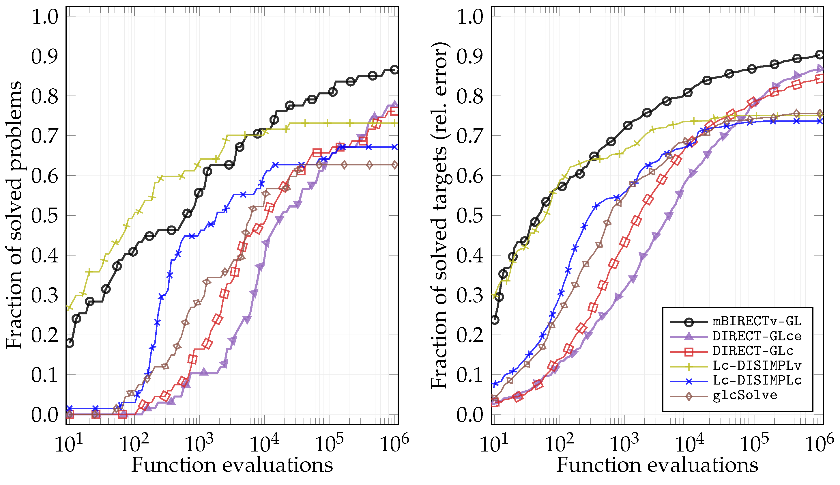
4.2. Analysis of the Overall Performance of Algorithms

Table 1. Performance evaluation of DIRECT-type algorithms on 67 linearly constrained optimization problems.

		Average Number of Function Evaluations
Algorithm	Fails	Overall	$\mathit{n}\le 5$	$\mathit{n}\ge 6$	AC 1	NAC 2
mBIRECTv-GL	$9/67$	$\mathrm{155,031}$	$\mathrm{70,140}$	$\mathrm{340,980}$	$\mathrm{107,449}$	$\mathrm{294,975}$
Lc-DISIMPLv	$18/67$	$\mathrm{269,349}$	$\mathrm{66,192}$	$\mathrm{714,356}$	$\mathrm{260,327}$	$\mathrm{295,882}$
Lc-DISIMPLc	$22/67$	$\mathrm{333,860}$	$\mathrm{137,852}$	$\mathrm{763,208}$	$\mathrm{396,432}$	$\mathrm{295,026}$
glcSolve	$23/67$	$\mathrm{370,703}$	$\mathrm{134,031}$	$\mathrm{889,126}$	$\mathrm{166,726}$	$\mathrm{572,827}$
DIRECT-GLc	$16/67$	$\mathrm{286,976}$	$\mathrm{114,737}$	$\mathrm{664,259}$	$\mathrm{281,871}$	$\mathrm{301,988}$
DIRECT-GLce	$14/67$	$\mathrm{283,836}$	$\mathrm{121,677}$	$\mathrm{639,040}$	$\mathrm{277,607}$	$\mathrm{302,154}$

¹ Problems with active constraints; ² Problems without active constraints.

summarizes the experimental results obtained from six algorithms. The second column shows the number of problems that were not solved within the specified relative error, while columns three to seven display the average number of function evaluations for different subsets of problems.

Among the algorithms analyzed, our new mBIRECTv-GL algorithm demonstrated the highest success rate, with only 9 of the 67 problems remaining unsolved. The DIRECT-GLce algorithm and the DIRECT-GLc algorithm closely followed, with 14 and 16 unsolved problems, respectively, placing them as the second and third most effective algorithms.

When considering the overall average of function evaluations, the algorithm mBIRECTv-GL outperformed all other algorithms, showing nearly twice the effectiveness of the second-best algorithm, Lc-DISIMPLv. However, for problems with smaller dimensions ($n\le 5$), the Lc-DISIMPLv algorithm displayed the best average results. Although our mBIRECTv-GL required approximately $6\%$ more function evaluations compared to Lc-DISIMPLv, it outperformed the latter by requiring about $52\%$ fewer evaluations for larger-dimensional ($n\ge 6$) problems.

The final two columns display the average number of function evaluations for problems with and without active constraints. When none of the constraint functions are active, most algorithms exhibit similar performance, except for the glcSolve algorithm, which shows comparatively inferior results in such cases (see column NAC). However, when the solution lies on the boundary of the feasible region, our developed algorithm exhibits a clear advantage (see column AC).

Figure 6 presents the data profiles [61,62] and empirical cumulative distributions (ECD) using the entire dataset considered. To construct the ECD, we established 51 targets with relative precisions ranging from ${10}^{[2,\dots ,-2]}$ (a similar setup as in [63]). These ECD plots, as exemplified on the right-hand side of Figure 6, provide information on the performance of the algorithms in different search stages. Both the data profiles and the ECD plots highlight the dominance of two algorithms, mBIRECTv-GL and Lc-DISIMPLv. This is attributed to their sampling strategy, which directly samples points on the boundaries. mBIRECTv-GL and Lc-DISIMPLv exhibit higher success rates while requiring fewer function evaluations, making them more efficient and cost-effective than other algorithms.

The data profiles displayed on the left side of Figure 6 indicate that within a small evaluation budget (≤4$\times {10}^3$), the Lc-DISIMPLv algorithm is slightly more efficient than our algorithm developed and can solve a greater number of test problems. However, the ECD plot on the right side of Figure 6 reveals that these algorithms solve similar percentages of target errors within ≤3$\times {10}^2$. When larger evaluation budgets are considered, the mBIRECTv-GL algorithm outperforms all other algorithms.

4.3. Statistical Analysis of the Results

The validity of the results and comparisons between algorithms and the significance of the improvements achieved by mBIRECTv-GL were evaluated using the non-parametric Wilcoxon signed test at a significance level of $5\%$. A p-value greater than $0.05$ suggests that the difference in results between the two methods is insignificant.

Table 2. p-values of the Wilcoxon signed test with $5\%$ significance, mBIRECTv-GL vs. other competitors, using different objective function evaluation budgets.

Algorithm	${10}^2$	${10}^3$	${10}^4$	${10}^5$	${10}^6$
Lc-DISIMPLv	$4.3758\times {10}^{-3}$	$4.1523\times {10}^{-3}$	$1.0205\times {10}^{-3}$	$2.9316\times {10}^{-4}$	$2.1367\times {10}^{-4}$
Lc-DISIMPLc	$7.2762\times {10}^{-9}$	$2.8887\times {10}^{-5}$	$1.8188\times {10}^{-4}$	$6.3294\times {10}^{-5}$	$8.0517\times {10}^{-5}$
glcSolve	$1.4166\times {10}^{-7}$	$8.7745\times {10}^{-6}$	$4.8968\times {10}^{-5}$	$1.4354\times {10}^{-3}$	$1.1472\times {10}^{-4}$
DIRECT-GLc	$3.5571\times {10}^{-11}$	$2.2431\times {10}^{-9}$	$2.6512\times {10}^{-5}$	$1.1858\times {10}^{-3}$	$1.4097\times {10}^{-2}$
DIRECT-GLce	$4.2110\times {10}^{-11}$	$4.5098\times {10}^{-10}$	$7.0552\times {10}^{-7}$	$2.4254\times {10}^{-4}$	$3.9474\times {10}^{-2}$

displays the p-values obtained comparing mBIRECTv-GL with other DIRECT-type competitor solvers. For all instances, the p-values are below $0.05$, which indicates that mBIRECTv-GL exhibits significantly superior performance compared to other techniques and surpasses the performance of other algorithms for the benchmark problems examined. However, as the evaluation budgets increase, the p-values of the penalty-based DIRECT-type algorithms closely approach the $5\%$ significance level.

Taking into account the results of the Friedman mean rank test presented in

Table 3. Friedman mean rank values, using different objective function evaluation budgets.

Algorithm	${10}^2$	${10}^3$	${10}^4$	${10}^5$	${10}^6$
mBIRECTv-GL	$1.8060$	$2.2015$	$2.6866$	$2.8806$	$2.9030$
Lc-DISIMPLv	$2.4478$	$2.9179$	$3.3060$	$3.7164$	$3.7910$
Lc-DISIMPLc	$4.0373$	$3.5373$	$3.7537$	$3.9552$	$3.9701$
glcSolve	$3.3134$	$3.1866$	$3.4851$	$3.5672$	$3.8059$
DIRECT-GLc	$4.5672$	$4.1866$	$3.5224$	$3.3731$	$3.2761$
DIRECT-GLce	$4.8284$	$4.9701$	$4.2463$	$3.5075$	$3.1567$
p-value	$8.4848\times {10}^{-32}$	$2.5717\times {10}^{-23}$	$3.1391\times {10}^{-9}$	$7.3195\times {10}^{-6}$	$3.3810\times {10}^{-9}$

, mBIRECTv-GL achieves the highest ranking among the approaches for all budgets for the evaluation of objective functions. The developed algorithm is most advantageous when smaller evaluation budgets are used. The Friedman test, conducted at a level of significance $5\%$, indicates a significant difference in the performance of the various algorithms. Nevertheless, as the evaluation budgets are raised, the Friedman mean rank values exhibit decreased dispersion, implying that there will come the point where the algorithms will demonstrate similar performance.

5. Conclusions and Future Prospects

This paper adds a novel approach to the class of DIRECT-type algorithms. The proposed algorithm (mBIRECTv-GL) is specifically designed to tackle global optimization problems involving Lipschitz continuous functions subject to linear constraints. By integrating the most recent partitioning and selection techniques and applying mapping techniques to eliminate the infeasible region, the novel algorithm demonstrates remarkable efficiency and superior performance compared to the existing DIRECT counterparts.

Although existing solution techniques, such as simplicial partitioning approaches, operate exclusively within feasible regions, their effectiveness decreases significantly in larger dimensions. In contrast, penalty- and auxiliary-function-based approaches exhibit slower convergence rates and often require a considerably higher number of function evaluations due to their handling of large infeasible regions. These methods also face notable challenges when dealing with problems where the optimal solution lies precisely at the boundaries of feasibility.

To validate the effectiveness of our approach, we conducted extensive experimentation using a diverse set of benchmark problems. Our results highlight the superior performance of our algorithm, particularly when solutions are located at the boundary of feasible regions. The statistical analyses, including the Friedman and Wilcoxon tests, further support our results.

This research opens up novel possibilities for addressing Lipschitz-continuous optimization problems with linear constraints, providing an improved algorithmic solution with enhanced computational efficiency. Therefore, the new algorithm will have an important place among all other DIRECT-type algorithms available in the open-source DIRECTGO repository (see the Data Availability Statement below). To achieve even greater usability, as a potential direction, we consider integrating DIRECT-type algorithms into the new web-based tool for algebraic modeling and mathematical optimization [64,65]. Alternatively, at least the most efficient DIRECT-type algorithms could be hosted on the NEOS Server (https://neos-server.org/neos/, (accessed on 30 May 2023))—a free internet-based service for solving numerical optimization problems.

References

1. Lucidi, S.; Sciandrone, M. A Derivative-Free Algorithm for Bound Constrained Optimization. Comput. Optim. Appl. 2002, 21, 119–142. [Google Scholar] [CrossRef]
2. Giovannelli, T.; Liuzzi, G.; Lucidi, S.; Rinaldi, F. Derivative-free methods for mixed-integer nonsmooth constrained optimization. Comput. Optim. Appl. 2022, 82, 293–327. [Google Scholar] [CrossRef]
3. Kimiaei, M.; Neumaier, A. Efficient unconstrained black box optimization. Math. Program. Comput. 2022, 14, 365–414. [Google Scholar] [CrossRef]
4. Holland, J. Adaptation in Natural and Artificial Systems; The University of Michigan Press: Ann Arbor, MI, USA, 1975. [Google Scholar]
5. Eberhart, R.; Kennedy, J. A new optimizer using particle swarm theory. In Proceedings of the Sixth International Symposium on Micro Machine and Human Science (MHS’95), Nagoya, Japan, 4–6 October 1995; pp. 39–43. [Google Scholar] [CrossRef]
6. Kirkpatrick, S.; Gelatt, C.D.; Vecchi, M.P. Optimization by simulated annealing. Science 1983, 220, 671–680. [Google Scholar] [CrossRef]
7. Bujok, P.; Kolenovsky, P. Eigen crossover in cooperative model of evolutionary algorithms applied to cec 2022 single objective numerical optimisation. In Proceedings of the 2022 IEEE Congress on Evolutionary Computation (CEC), Padua, Italy, 18–23 July 2022; pp. 1–8. [Google Scholar] [CrossRef]
8. Hadi, A.A.; Mohamed, A.W.; Jambi, K.M. Single-objective real-parameter optimization: Enhanced LSHADE-SPACMA algorithm. Heuristics Optim. Learn. 2021, 906, 103–121. [Google Scholar] [CrossRef]
9. Paulavičius, R.; Stripinis, L.; Sutavičiūtė, S.; Kočegarov, D.; Filatovas, E. A novel greedy genetic algorithm-based personalized travel recommendation system. Expert Syst. Appl. 2023, 230, 120580. [Google Scholar] [CrossRef]
10. Jones, D.R.; Schonlau, M.; Welch, W.J. Efficient Global Optimization of Expensive Black-Box Functions. J. Glob. Optim. 1998, 13, 455–492. [Google Scholar] [CrossRef]
11. Björkman, M.; Holmström, K. Global Optimization of Costly Nonconvex Functions Using Radial Basis Functions. Optim. Eng. 2000, 1, 373–397. [Google Scholar] [CrossRef]
12. Lera, D.; Sergeyev, Y.D. Lipschitz and Hölder global optimization using space-filling curves. Appl. Numer. Math. 2010, 60, 115–129. [Google Scholar] [CrossRef]
13. Sergeyev, Y.D.; Kvasov, D.E. Lipschitz global optimization. In Wiley Encyclopedia of Operations Research and Management Science (in 8 Volumes); Cochran, J.J., Cox, L.A., Keskinocak, P., Kharoufeh, J.P., Smith, J.C., Eds.; John Wiley & Sons: New York, NY, USA, 2011; Volume 4, pp. 2812–2828. [Google Scholar]
14. Martins, J.R.R.A.; Ning, A. Engineering Design Optimization; Cambridge University Press: Cambridgem, UK, 2021. [Google Scholar]
15. Best, M.J. Portfolio Optimization; CRC Press: Boca Raton, FL, USA, 2010. [Google Scholar]
16. Floudas, C.A.; Pardalos, P.M.; Adjiman, C.; Esposito, W.R.; Gümüs, Z.H.; Harding, S.T.; Klepeis, J.L.; Meyer, C.A.; Schweiger, C.A. Handbook of Test Problems in Local and Global Optimization; Springer: Berlin/Heidelberg, Germany, 2013; Volume 33. [Google Scholar]
17. Jones, D.R.; Perttunen, C.D.; Stuckman, B.E. Lipschitzian Optimization Without the Lipschitz Constant. J. Optim. Theory Appl. 1993, 79, 157–181. [Google Scholar] [CrossRef]
18. Jones, D.R. The Direct Global Optimization Algorithm. In The Encyclopedia of Optimization; Floudas, C.A., Pardalos, P.M., Eds.; Kluwer Academic Publishers: Dordrect, The Netherlands, 2001; pp. 431–440. [Google Scholar]
19. Jones, D.R.; Martins, J.R.R.A. The DIRECT algorithm: 25 years later. J. Glob. Optim. 2021, 79, 521–566. [Google Scholar] [CrossRef]
20. Sergeyev, Y.D.; Kvasov, D.E. Global search based on diagonal partitions and a set of Lipschitz constants. SIAM J. Optim. 2006, 16, 910–937. [Google Scholar] [CrossRef] [Green Version]
21. Holmstrom, K.; Goran, A.O.; Edvall, M.M. User’s Guide for TOMLAB 7. Technical Report. Tomlab Optimization Inc. 2010. Available online: https://tomopt.com/docs/TOMLAB.pdf (accessed on 15 June 2023).
22. Stripinis, L.; Žilinskas, J.; Casado, L.G.; Paulavičius, R. On MATLAB experience in accelerating DIRECT-GLce algorithm for constrained global optimization through dynamic data structures and parallelization. Appl. Math. Comput. 2021, 390, 125596. [Google Scholar] [CrossRef]
23. Stripinis, L.; Paulavičius, R. An empirical study of various candidate selection and partitioning techniques in the DIRECT framework. J. Glob. Optim. 2022, 1–31. [Google Scholar] [CrossRef]
24. Stripinis, L.; Paulavičius, R.; Žilinskas, J. Penalty functions and two-step selection procedure based DIRECT-type algorithm for constrained global optimization. Struct. Multidiscip. Optim. 2019, 59, 2155–2175. [Google Scholar] [CrossRef]
25. Stripinis, L.; Paulavičius, R. Experimental Study of Excessive Local Refinement Reduction Techniques for Global Optimization DIRECT-Type Algorithms. Mathematics 2022, 10, 3760. [Google Scholar] [CrossRef]
26. Stripinis, L.; Paulavičius, R. Lipschitz-inspired HALRECT algorithm for derivative-free global optimization. J. Glob. Optim. 2023, 1–31. [Google Scholar] [CrossRef]
27. Liuzzi, G.; Lucidi, S.; Piccialli, V. A direct-based approach exploiting local minimizations for the solution for large-scale global optimization problems. Comput. Optim. Appl. 2010, 45, 353–375. [Google Scholar] [CrossRef]
28. Liuzzi, G.; Lucidi, S.; Piccialli, V. Exploiting derivative-free local searches in direct-type algorithms for global optimization. Comput. Optim. Appl. 2016, 65, 449–475. [Google Scholar] [CrossRef]
29. Kvasov, D.E.; Mukhametzhanov, M.S. Metaheuristic vs. deterministic global optimization algorithms: The univariate case. Appl. Math. Comput. 2018, 318, 245–259. [Google Scholar] [CrossRef]
30. Rios, L.M.; Sahinidis, N.V. Derivative-free optimization: A review of algorithms and comparison of software implementations. J. Glob. Optim. 2013, 56, 1247–1293. [Google Scholar] [CrossRef] [Green Version]
31. Sergeyev, Y.D.; Kvasov, D.E.; Mukhametzhanov, M.S. On the efficiency of nature-inspired metaheuristics in expensive global optimization with limited budget. Sci. Rep. 2018, 8, 453. [Google Scholar] [CrossRef] [PubMed] [Green Version]
32. Costa, M.F.P.; Rocha, A.M.A.C.; Fernandes, E.M.G.P. Filter-based DIRECT method for constrained global optimization. J. Glob. Optim. 2018, 71, 517–536. [Google Scholar] [CrossRef]
33. Finkel, D.E. MATLAB Source Code for DIRECT. 2004. Available online: http://www4.ncsu.edu/~ctk/Finkel_Direct/ (accessed on 22 March 2017).
34. Liu, H.; Xu, S.; Chen, X.; Wang, X.; Ma, Q. Constrained global optimization via a DIRECT-type constraint-handling technique and an adaptive metamodeling strategy. Struct. Multidiscip. Optim. 2017, 55, 155–177. [Google Scholar] [CrossRef]
35. Pillo, G.D.; Liuzzi, G.; Lucidi, S.; Piccialli, V.; Rinaldi, F. A DIRECT-type approach for derivative-free constrained global optimization. Comput. Optim. Appl. 2016, 65, 361–397. [Google Scholar] [CrossRef] [Green Version]
36. Pillo, G.D.; Lucidi, S.; Rinaldi, F. An approach to constrained global optimization based on exact penalty functions. J. Optim. Theory Appl. 2010, 54, 251–260. [Google Scholar] [CrossRef]
37. Gablonsky, J.M. Modifications of the DIRECT Algorithm. Ph.D. Thesis, North Carolina State University, Raleigh, NC, USA, 2001. [Google Scholar]
38. Na, J.; Lim, Y.; Han, C. A modified DIRECT algorithm for hidden constraints in an LNG process optimization. Energy 2017, 126, 488–500. [Google Scholar] [CrossRef]
39. Stripinis, L.; Paulavičius, R. A new DIRECT-GLh algorithm for global optimization with hidden constraints. Optim. Lett. 2021, 15, 1865–1884. [Google Scholar] [CrossRef]
40. Paulavičius, R.; Žilinskas, J. Advantages of simplicial partitioning for Lipschitz optimization problems with linear constraints. Optim. Lett. 2016, 10, 237–246. [Google Scholar] [CrossRef]
41. Stripinis, L.; Paulavičius, R. DIRECTGOLib—DIRECT Global Optimization Test Problems Library. Version v1.3, Zenodo. 2023. Available online: https://zenodo.org/record/8046086/export/hx (accessed on 15 June 2023).
42. Friedman, M. The Use of Ranks to Avoid the Assumption of Normality Implicit in the Analysis of Variance. J. Am. Stat. Assoc. 1937, 32, 675–701. [Google Scholar] [CrossRef]
43. Hollander, M.; Wolfe, D. Nonparametric Statistical Methods, Solutions Manual; Wiley Series in Probability and Statistics; Wiley: Hoboken, NJ, USA, 1999. [Google Scholar]
44. Gablonsky, J.M.; Kelley, C.T. A locally-biased form of the DIRECT algorithm. J. Glob. Optim. 2001, 21, 27–37. [Google Scholar] [CrossRef]
45. Paulavičius, R.; Žilinskas, J. Analysis of different norms and corresponding Lipschitz constants for global optimization in multidimensional case. Inf. Technol. Control 2007, 36, 383–387. [Google Scholar]
46. Paulavičius, R.; Žilinskas, J. Simplicial Lipschitz optimization without the Lipschitz constant. J. Glob. Optim. 2014, 59, 23–40. [Google Scholar] [CrossRef]
47. Paulavičius, R.; Žilinskas, J. Simplicial Global Optimization; SpringerBriefs in Optimization; Springer: New York, NY, USA, 2014. [Google Scholar] [CrossRef]
48. Finkel, D.E. Global Optimization with the Direct Algorithm. Ph.D. Thesis, North Carolina State University, Raleigh, NC, USA, 2005. [Google Scholar]
49. Fletcher, R.; Leyffer, S. Nonlinear programming without a penalty function. Math. Program. 2002, 91, 239–269. [Google Scholar] [CrossRef]
50. Barber, C.B.; Dobkin, D.P.; Huhdanpaa, H. The quickhull algorithm for convex hulls. ACM Trans. Math. Softw. (TOMS) 1996, 22, 469–483. [Google Scholar] [CrossRef] [Green Version]
51. Becker, S. CON2VERT—Constraints to Vertices, MATLAB Central File Exchange. 2023. Available online: https://www.mathworks.com/matlabcentral/fileexchange/7894-con2vert-constraints-to-vertices (accessed on 16 May 2023).
52. Huyer, W.; Neumaier, A. Global Optimization by Multilevel Coordinate Search. J. Glob. Optim. 1999, 14, 331–355. [Google Scholar] [CrossRef]
53. Liu, H.; Xu, S.; Wang, X.; Wu, X.; Song, Y. A global optimization algorithm for simulation-based problems via the extended DIRECT scheme. Eng. Optim. 2015, 47, 1441–1458. [Google Scholar] [CrossRef]
54. Chiter, L. Experimental Data for the Preprint “Diagonal Partitioning Strategy Using Bisection of Rectangles and a Novel Sampling Scheme”. Mendeley Data, V2. 2023. Available online: https://data.mendeley.com/datasets/x9fpc9w7wh/2 (accessed on 16 June 2023).
55. Paulavičius, R.; Chiter, L.; Žilinskas, J. Global optimization based on bisection of rectangles, function values at diagonals, and a set of Lipschitz constants. J. Glob. Optim. 2018, 71, 5–20. [Google Scholar] [CrossRef]
56. Stripinis, L.; Paulavičius, R.; Žilinskas, J. Improved scheme for selection of potentially optimal hyper-rectangles in DIRECT. Optim. Lett. 2018, 12, 1699–1712. [Google Scholar] [CrossRef]
57. Finkel, D.E.; Kelley, C.T. Additive scaling and the DIRECT algorithm. J. Glob. Optim. 2006, 36, 597–608. [Google Scholar] [CrossRef]
58. Paulavičius, R.; Sergeyev, Y.D.; Kvasov, D.E.; Žilinskas, J. Globally-biased DISIMPL algorithm for expensive global optimization. J. Glob. Optim. 2014, 59, 545–567. [Google Scholar] [CrossRef]
59. Stripinis, L.; Paulavičius, R. DIRECTGO: A New DIRECT-Type MATLAB Toolbox for Derivative-Free Global Optimization. ACM Trans. Math. Softw. 2022, 48, 41. [Google Scholar] [CrossRef]
60. Paulavičius, R.; Sergeyev, Y.D.; Kvasov, D.E.; Žilinskas, J. Globally-biased BIRECT algorithm with local accelerators for expensive global optimization. Expert Syst. Appl. 2020, 144, 11305. [Google Scholar] [CrossRef]
61. Moré, J.J.; Wild, S.M. Benchmarking derivative-free optimization algorithms. SIAM J. Optim. 2009, 20, 172–191. [Google Scholar] [CrossRef] [Green Version]
62. Grishagin, V.A. Operating characteristics of some global search algorithms. In Problems of Stochastic Search; Zinatne: Riga, Latvia, 1978; Volume 7, pp. 198–206. (In Russian) [Google Scholar]
63. Hansen, N.; Auger, A.; Ros, R.; Mersmann, O.; Tušar, T.; Brockhoff, D. COCO: A platform for comparing continuous optimizers in a black-box setting. Optim. Methods Softw. 2021, 36, 114–144. [Google Scholar] [CrossRef]
64. Jusevičius, V.; Oberdieck, R.; Paulavičius, R. Experimental Analysis of Algebraic Modelling Languages for Mathematical Optimization. Informatica 2021, 32, 283–304. [Google Scholar] [CrossRef]
65. Jusevičius, V.; Paulavičius, R. Web-Based Tool for Algebraic Modeling and Mathematical Optimization. Mathematics 2021, 9, 2751. [Google Scholar] [CrossRef]
66. Vaz, A.; Vicente, L. Pswarm: A hybrid solver for linearly constrained global derivative-free optimization. Optim. Methods Softw. 2009, 24, 669–685. [Google Scholar] [CrossRef]
67. Horst, R.; Pardalos, P.M.; Thoai, N.V. Introduction to Global Optimization; Nonconvex Optimization and Its Application; Kluwer Academic Publishers: Berlin, Germany, 1995. [Google Scholar]
Figure 1. Illustration of the transformation.
Mathematics 11 02920 g001
Figure 2. Mapping the set D to D feas : An illustrative example using Horst1 test problem (see Appendix A, Table A1 for a reference and description of the problem).
Mathematics 11 02920 g002
Figure 3. Two-dimensional illustration on Horst1 test problem of sampling and bisection techniques employed in the extended version (BIRECTv [54]) of the original BIRECT algorithm [55]. The region enclosed by the black boundary represents D feas , whereas the red contours depict D D feas .
Mathematics 11 02920 g003
Figure 4. Application of the mapping technique embedded in the BIRECTv algorithm on Horst1 test problem. The region enclosed by the black boundary represents D feas .
Mathematics 11 02920 g004
Figure 5. An illustrative example of two algorithms: BIRECTv vs. BIRECTv with mapping techniques applied to the Horst1 test problem.
Mathematics 11 02920 g005
Figure 6. Data profiles and empirical cumulative distributions (ECD) of function evaluations for various target precisions on all problems.
Mathematics 11 02920 g006