The Set Covering and Other Problems: An Empiric Complexity Analysis Using the Minimum Ellipsoidal Width

Abstract

This research aims to explain the intrinsic difficulty of Karp’s list of twenty-one problems through the use of empirical complexity measures based on the ellipsoidal width of the polyhedron generated by the constraints of the relaxed linear programming problem. The variables used as complexity measures are the number of nodes visited by the $B\&B$ and the CPU time spent solving the problems. The measurements used as explanatory variables correspond to the Dikin ellipse eigenvalues within the polyhedron. Other variables correspond to the constraint clearance with respect to the analytical center used as the center of the ellipse. The results of these variables in terms of the number of nodes and CPU time are particularly satisfactory. They show strong correlations, above 60%, in most cases.

1. Introduction

The NP-completeness of Karp’s 21 problems list dates back to 1972 [1]. It is a list of classical problems that meet computational complexity characteristics. Some of the list’s problems solved in this paper included the set covering problem, the set packaging problem, the knapsack multi-demand problem, and some general integer programming problems. There were statistically significant relationships between the branching and bound tree number of nodes and the resolution time. Explanatory variables included geometric measurements corresponding to an inner Dikin ellipse that replicates the shape of the linear polyhedron. The test problems used are classics in combinatorics, computer science, and computational complexity theory.

The set covering problem, also known as SCP, is an NP-complete class problem. Solutions to these problems usually consist of finding a solution set to cover, totally or partially, a set of needs at the lowest possible cost. In many cases, the distance or the response time between customers and service delivery points is critical to customer satisfaction. For example, if a building catches fire, the fire station response time is vital; the longer the delay, the greater the building damage. In this case, the SCP model ensures that at least one fire station is at a close enough distance in order for fire engines to reach the building within a certain time. Set packing is also a classic problem. It consists of packaging sets of disjoint k subsets. The problem is visibly an NP problem because, given k subsets, subsets are disjoint 2 to 2 in polynomial time [2,3]. The optimization problem consists of finding the maximum number of sets, from 2 to 2 disjoints in a list. It is a maximization problem formulated as a packaging integer programming problem, and its dual linear problem is the set cover problem [4]. The multi-dimensional knapsack (MKP) problem involves selecting a set of items to carry in a knapsack subject to one or more restrictions. These may be the knapsack weight or volume. The objective function of this problem seeks to maximize a linear function in 0–1 variables subject to knapsack constraints. Finally, the multi-dimensional and multi-demand knapsack problem is the multi-dimensional knapsack problem to which added compliance restrictions present some demand conditions [5]. The CPU time is key when solving an MIP/BIP problem using the branch and bound ($B\&B$) algorithm. It depends on the search tree size associated with the algorithm. $B\&B$ finds the solution by recursively dividing the search space. The space is a tree where the root node is associated with the integer solution space. The brother nodes are a solution space partition of the parent node. At each node, the subspace is an MIP/BIP and its linear programming (LP) relaxation is solved to supply a linear solution. If the LP is not workable or better than the primary solution (the best integer value found), the procedure prunes the node. A previous article proposed complexity indices to estimate the $B\&B$ tree size, which applies to the multi-dimensional backpack problem [6].

1.1. $B\&B$ Tree Counting Literature Review

Knuth [7] proposed the first method to estimate the search tree size of the branch and bound ($B\&B$) algorithm. This method works by repeatedly sampling the search tree sequence and estimating a measure of the node number to disaggregate. This calculates the $B\&B$ tree by repeatedly following random paths from the root. As the search may prove to be extensive, Purdom [8] improved the method by following more than one path from a node. Tree size was estimated by performing a partial backtracking search. This modification exponentially improves results with the tree height. Purdom called this method Partial Backtracking. Chen [9] improved Knuth’s proposed method using heuristic sampling to estimate its efficiency. This updated version produces significantly higher efficiency estimates for tree search strategies commonly used. These are depth first, breadth first, best first, and iterative deepening. Belov et al. [10] combined Knuth’s sampling procedure with the abstract $B\&B$ tree developed by Le Bodic and Nemhauser [11]. Knuth’s original method uses the distribution of node knowledge in a $B\&B$ tree by reducing the variance in tree size estimates, while Le Bodic and Nemhauser provide a theoretical $B\&B$ tree model. Belov et al. combined these two methods to obtain a significant estimation accuracy increase. According to Belov et al. and the conducted experiments, the error decreased by more than half in the a priori estimation. The abstract tree developed by Le Bodic and Nemhauser [11] is a formula based on the concept of gain by branching into any node. They use an a priori estimate of the gain obtained by branching left or right into any node. They also use what they call gap, which is the gain value that allows for obtaining the optimal integer solution via branching. Their use of the abstract tree seeks to find the best variable to branch, i.e., to obtain a tree of minimum size. Other estimation methods are the Weighted Backtrack Estimator [12], Profile Estimation [13], and the Sum of Subtree Gaps [14]. Recently, Refs. [15,16,17] developed methods based on machine learning in the context of integer programming. Fischetti in [18] proposed a classifier to predict specific points online. Finally, Hendel et al. [19] developed a new version of the old method of estimating the $B\&B$ tree. They integrated Le Bodic and Nemhauser’s [11] theoretical tree and new measures such as "leaf frequency". A leaf in the $B\&B$ tree is a node that does not dis-aggregate, and this may be because it delivers an integer solution, which is unfeasible or needs pruning. They then use this and other measures of algorithm progress using machine learning’s random forest model to estimate the size of the $B\&B$ tree. Next, they integrate this technique into the SCIP constrained integer programming software [20]. The application of these methods occurs throughout the algorithm, since they require a few iterations to start with the estimate, and there are iterations for recalculations. Its accuracy also grows as the algorithm progresses, and so does the availability of information.

1.2. Our Contribution to the Problem of Estimating the B&B Tree

Our estimation of the $B\&B$ tree research line, including the methods developed in this work, follows the conditioning concept in integer programming [21,22,23]. Vera and Derpich [24] proposed dimensions for the polyhedron width, based on m (number of constraints) and n (number of variables). The dimension used is to estimate the number of upper bounds of iterations of the $B\&B$ algorithm and the Lenstra algorithm [25]. Vera and Derpich also proposed two measures concerning the polyhedron ellipsoidal width, which are the maximum slack and a term called the “distance to ill-posedness of the integer problem”, which Vera documented in [22]. The number of iterations of the $B\&B$ algorithm’s proposed dimensions [25] corresponds to worst-case dimensions. They are similar when compared with those proposed by Le Bodic and Nemhauser [11], since both give values far from the real values obtained. Vera and Derpich’s [22] proposed dimensions basis includes concepts that reflect the shape and spatial orientation of the polyhedron. Earlier approaches do not capture these factors. Therefore, these dimensions also predict the $B\&B$ tree node number and CPU time. These are the conceptual basis of this work. The indices developed in this work use a Dikin ellipse inside the polyhedron. They show a good correlation with the $B\&B$ algorithm CPU time and the number of nodes visited. The Dikin ellipse allows for the estimation of the polyhedron ellipsoidal width, which iterates n times to estimate the $B\&B$ tree. This enables applications to new, related geometric indices, starting with the constraints of the linear programming problem generated by relaxing the integer variables. The proposed indices’ basis is the concept of polyhedron flatness. This means that if a polyhedron is thin in some direction, the $B\&B$ algorithm might run faster. In this article, we seek to test how much this idea influences the $B\&B$ tree size, characterized by the number of nodes visited and the CPU time. The underlying conjecture for the proposed experimental design is that a narrower polyhedron will be faster to cross. Therefore, the $B\&B$ tree will be smaller and vice versa, i.e., in a narrower polyhedron, the $B\&B$ tree will be larger. These new factors are related to the dimensions of the matrices associated with the polyhedron of the relaxed problem, as well as the maximum and minimum slacks with respect to the center of the ellipse. To test the relationship between these measures and the $B\&B$ tree’s number of nodes, we designed an experimental study and found a strong linear correlation. The empirical study included set covering, set packing, and other general problems of integer programming. Data came from the public library MIPLIB [26,27,28]. We also assessed the multi-demand multi-dimensional knapsack (MDMKP) problem. Data were taken from OR-Library [28].

Following this introduction, and because they support the proposed complexity indices, Section 2 develops the concepts related to the polyhedron ellipsoidal width. Section 3 presents the problems under study in mathematical formulations, which are set covering, set packing, and multi-demand multi-dimensional backpack. Section 4 presents the experimental design, detailing the test problems used and the results obtained. Section 5 presents a discussion in which the work is compared with others that are similar in some way, and, finally, Section 6 summarizes the main findings and future work.

2. Methods and Materials

Polyhedron Ellipsoidal Width

Let K be a convex set in which $R^n$; we define the integer width of K as follows:

$$w_z\left(K\right)=w(v,K)$$

(1)

$$w(v,K)=\{v^{T}x:x\in K\}-\{v^{T}x:x\in K\}$$

(2)

If we restrict the vectors v to the Euclidean space set of unit vectors, with a unitary norm, we obtain the total width according to the coordinate axes $\{x_1,x_2,\dots ,x_n\}$. The integer width is a very interesting geometric measure. It is related to the existence of at least one integer point. If there is at least one integer point, this width cannot be too small. This is an important result because [29] stated that $w_Z\left(K\right)\le f\left(n\right)$ if K does not contain an integer point. Lenstra considered $f\left(n\right)$ to be of the order of $c_o^{n2}$, where $c_0$ is a constant. The problem approach that we study in this paper is as follows.

$$\max :\{c^{T}x:Ax\le b,x\ge 0,x\in Z^n\}$$

(3)

We assume that the polyhedron given by $Ax\le b$ is bounded and denotes the problem data with the letter d, so that $d=(A,b)\in R^{mxn+m}$. This is the problem-specific instance. We denote by $P\left(d\right)$ the $\{x:Ax\le b\}$ polyhedron, and by ${\alpha }_1$,…,${\alpha }_m$,$\{x:Ax\le b\}$ the row vectors of A. Next, we analyze an application of Lenstra’s flatness theorem [30]. We obtain a dimension that depends on geometry rather than dimensional factors. As in the classical flatness theorem analysis, the basis of the estimate lies in rounding the polyhedron using inscribed and circumscribed ellipses. Ellipses are intended to interpret the polyhedron shape with certainty. Therefore, let us build a pair of ellipses with a common center $x^0$.

$$E=\{x\in R^n:{(x-x^0)}^{T}Q(x-x_0)\le 1\}$$

(4)

and

$$E^{\prime }=\{x\in R^n:{(x-y)}^{T}Q(x-y)\le {\gamma }^2\}$$

(5)

so that

$$E\subset P\left(d\right)\subset E^{\prime }$$

(6)

where Q is a definite positive matrix. The matrices have different possibilities, depending on the value of $\gamma$. John proposes [31] an ellipse $E’$ with minimal volume by making $\gamma =n$ However, computing $x^0$ becomes a hard problem. We use an approach based on the classic setup of interior point methods in convex linear optimization [32]. Suppose that we know a self-concordant barrier function $\mathsf{\Phi }$, on a convex body, with parameter v as in Nesterov and Nemirosky [33]. Then, let

$$x_0=argmin\{\mathsf{\Phi }\left(x\right):x\in int P\left(d\right)\}$$

(7)

Let $Q={\nabla }^2\mathsf{\Phi }\left(x^0\right)$ and E be a unit radius inner ellipse, known as a Dikin ellipse. Thus, if we take $\gamma =m+1$, for example, we use the traditional logarithmic barrier function

$$\mathsf{\Phi }\left(x\right)=-{\sum }_{i=1}^{n}log(b_i-{\alpha }_i^{t}x),$$

with $v=m$. The point $x^0$ is the $K=P\left(d\right)$ analytical center and the matrix Q is

$$Q=A^{T}D{\left(x^0\right)}^{-2}A$$

(8)

with

$$D\left(x\right)=diag(b_1-{\alpha }_1^{T}x,b_2-{\alpha }_2^{T}x,\dots ,b_m-{\alpha }_m^{T}x)$$

(9)

where $diag\left(\right)$ denotes a diagonal matrix constructed with the corresponding elements. The fact that the matrix Q naturally connects with the polyhedron’s geometric properties justifies the ellipsis construction choice. The following is the ellipses’ geometrical result.

Proposition 1. 

Let Q be a positively defined symmetric real matrix by defining a pair of ellipses as in (4). Then,

$$W_z\left(P\left(d\right)\right)\le 2(m+1)\sqrt{min\left(u^t{Q}^{-1}u\right):uϵZ^n,u\ne 0}$$

(10)

Demonstration.

The term $\sqrt{min\left(u^t{Q}^{-1}u\right)}$ is ellipse E’s radius, according to the direction u.

2$\sqrt{min\left(u^t{Q}^{-1}u\right)}$ is the ellipse E’s width, according to vector u.

Multiplying by $(m+1)$, we obtain the expanded ellipse $E^{\prime }$.

Then, 2$\sqrt{min\left(u^t{Q}^{-1}u\right)}$ is ellipse $E^{\prime }$’s width, according to the vector u.

The value 2$\sqrt{min\left(u^t{Q}^{-1}u\right)}$ is greater than the polyhedron $P\left(d\right)$’s width, according to vector $u■$.

Proposition 2. 

Let $v_1,\dots ,v_n$ be the positive definite matrix Q orthonormal eigenvectors, and ${\lambda }_{min}$ be the smallest eigenvalue of Q. Then, for any $u\in R^n$,

$$u^T{Q}^{-1}u\le \left(\frac{1}{{\lambda }_{min}}\right)\sum _{i=1}^n{v}_i^T{u}^2$$

(11)

Demonstration.

Since Q is symmetric and defined as positive, the result comes from the fact that

$$Q^{-1}={\sum }_{i=1}^n\frac{1}{{\lambda }_i}{v}_i{v}_i^T$$

It follows that

$$u^T{Q}^{-1}u={\sum }_{i=1}^n\frac{1}{{\lambda }_i}{\left(u^T{v}_i\right)}^2$$

Then, taking the minimum eigenvalue, we have

$$u^T{Q}^{-1}u\le {\sum }_{i=1}^n\frac{1}{{\lambda }_{min}}{v}_i^T{u}^2■$$

Because we use it in our analysis, we describe the result of Vera [22], which relates the matrix Q eigenvalues to the matrix $A^{T}A$ eigenvalues and other data.

Proposition 3. 

Let $Q=A^{T}D{\left(x^0\right)}^{-2}A$ with $D\left(x\right)=diag(b_1-{\alpha }_1^{T}x,\dots ,b_n-{\alpha }_m^T),b_i-{\alpha }_i^T>0,i=1,\dots ,m.$ Let ${\lambda }_{min}$ and ${\lambda }_{max}$ be the smallest and largest Q eigenvalues, respectively. Let ${\mu }_{min}$ and ${\mu }_{max}$ be the smallest and largest $A^{T}A$ eigenvalues, respectively. Additionally, let $h_{max}$ be the highest and lowest $D\left(x\right)$ values. Then, it fulfills

$${\lambda }_{min}\ge \frac{{\mu }_{min}}{{\left(h_{max}\left(x^0\right)\right)}^2}$$

(12)

$${\lambda }_{max}\ge \frac{{\mu }_{max}}{{\left(h_{min}\left(x^0\right)\right)}^2}$$

(13)

Demonstration [22,24].

Proposition 4. 

Let ${\lambda }_i$ and $v_i$ be the matrix Q eigenvalues and eigenvectors, respectively, $i=1,\dots ,n$ Let u be a possible solution. Then, we have the following:

$$w(u,P\left(d\right))\le 2(m+1){\parallel v_{max}\parallel }_2\frac{h_{max}\left(x^0\right)}{\sqrt{u_{min}}}$$

(14)

Demonstration.

From Proposition 1’s demonstration, we have

$$W_z\left(P\left(d\right)\right)\le 2(m+1)\sqrt{min\left(u^t{Q}^{-1}u\right):uϵZ^n,u\ne 0}$$

(15)

From Proposition 2, we have

$$u^T{Q}^{-1}u\le \left(\frac{1}{{\lambda }_{min}}\right)\sum _{i=1}^n{v}_i^T{u}^2$$

(16)

Taking an upper bound with a norm-2 higher eigenvector, we have

$$\sum _{i=1}^n{\left(v_i^{T}u\right)}^2\le \sum _{i=1}^n{\left(v_{max}^{T}u\right)}^2$$

(17)

Assuming that ${\parallel u\parallel }_{\infty }\le 1$, then

$$\sum _{i=1}^n{\left(v_i^{T}u\right)}^2\le \sum _{i=1}^n{\left(v_{max}^{T}u\right)}^2\le {\parallel v_{max}\parallel }_2^2$$

(18)

Additionally, from Proposition 3, we have

$$\frac{1}{{\lambda }_{min}}\le \frac{{\left(h_{max}\left(x^0\right)\right)}^2}{u_{min}}$$

(19)

$$w(u,P\left(d\right))\le 2(m+1)\sqrt{\left(\frac{1}{{\lambda }_{min}}\right)\sum _{i=1}^n{\left(v_i^{T}u\right)}^2}\le 2(m+1)\frac{h_{max}\left(x^0\right)}{\sqrt{u_{min}}}{\parallel v_{max}\parallel }_2■$$

(20)

In a previous paper, Ref. [34] built a disjunction to branch variables in the $B\&B$, based on the associated linear polyhedron ellipsoidal. This simultaneously branches various variables, as if it was a super ruler that uses ellipsoidal width $u^T{Q}^{-1}u$. This rule proved to be more efficient than the known strong branching rule. The latter often leads to a smaller search tree, although it requires much more time to select branching variables. Figure 1 shows the ellipses used, in an exponential rounding approach, where Q is a positive definite matrix. This is a shortest vector problem version. Micciancio [35] considers it a difficult problem. We use Proposition 4 as a dimension only. Therefore, we do not solve it optimally. However, we use an upper bound of the optimal value, which captures some aspects of the original problem that reproduce the intrinsic difficulty of a particular instance. Based on Proposition 4, we propose the next dimension related to polyhedron $P\left(d\right)$’s geometry.

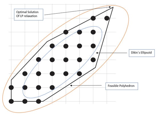
Figure 1. Ellipsoidal rounding using a pair of Dikin ellipses.

3. Experimental Design

This section describes the experimental design and shows the mathematical structure of the test problem considered, which is part of Karp’s list. The previous section found the variables related to geometric aspects. On this basis, a linear search established relationships between these variables. Additionally, two measures were related to the $B\&B$ tree, which were the number of explored nodes and the algorithm’s CPU time. Thus, the relationship searching work is fully experimental, and the results relate to the test problems only. They are not generalizable to other cases without re-running a similar experiment. The statistical model employed is a multiple regression model that uses the ANOVA test, using the F statistic to validate the overall model significance. The explained variables are the following:

• The solved instance CPU time, using the $B\&B$ algorithm.
• The number of nodes scanned by the $B\&B$ algorithm.

The explanatory variables studied were $x_i,i=1,2,3,4,5,6$ as follows:

• ${\lambda }_{max}\left(Q\right)$ is the maximum eigenvalue of the matrix $Q=A^{T}H{\left(xo\right)}^{-2}A$;
• ${\lambda }_{min}\left(Q\right)$ is the minimum eigenvalue of the matrix $Q=A^{T}H{\left(xo\right)}^{-2}A$;
• ${\mu }_{max}$ is the maximum eigenvalue of the matrix $A^{T}A$;
• ${\mu }_{min}$ is the minimum eigenvalue of the matrix $A^{T}A$;
• $h_{max}\left(x^0\right)=ma{x}_i\{b_i-{\alpha }_i^T{x}^0\}$ is the maximum slack to the center $x^0$;
• $h_{min}\left(x^0\right)=mi{n}_i\{b_i-{\alpha }_i^T{x}^0\}$ is the minimum slack to the center $x^0$.

We constructed two multiple regression models, named Model 1 and Model 2. The first uses the CPU time as the explained variable. The second model uses the number of nodes as the explained variable. The models are as follows:

Model 1: Number of nodes = ${\beta }_0+{\beta }_1{x}_1+{\beta }_2{x}_2+{\beta }_3{x}_3+{\beta }_4{x}_4+{\beta }_5{x}_5+{\beta }_6{x}_6$

Model 2: CPU time = ${\beta }_0+{\beta }_1{x}_1+{\beta }_2{x}_2+{\beta }_3{x}_3+{\beta }_4{x}_4+{\beta }_5{x}_5+{\beta }_6{x}_6$

3.1. Used Test Problems

3.1.1. The Set Covering Problem

This problem seeks to find the minimum number of variables with which to cover all sets at least once. [35,36] provided a formal definition. Let us look at this problem through an example. Suppose that we must cover with antennas a set of geographical areas in a city. Then, we define $x_j$ as a binary variable, i.e., 1 if an antenna is located in the area and 0 otherwise. Installing an antenna in area j has the cost $c_j\ge 0$ and $c_j\in R^n$. There are n geographical areas. Then, $j=1,\dots ,n$. Formally, the set covering problem is expressed as follows:

$$minz=\sum _{j=1}^n{c}_j{x}_j$$

(21)

subject to

$$\sum _{j=1}^n{x}_j\ge 1,\forall j$$

(22)

$$x_j=\{\begin{array}{c}1ifanantennaisintheareaj\\ 0otherwise\end{array}$$

(23)

$M_j$: areas served by an antenna located in area J.

3.1.2. The Set Packing Problem

Varizani [36] formulated the maximum set packing integer linear program as follows:

$$max=\sum _{s\in S}{x}_S$$

(24)

subject to

$$\sum _{s\in S}{x}_S\le 1\forall e\in U$$

(25)

$$x_S\in \{0,1\}s\in S$$

(26)

where U is the cover set.

3.1.3. The Multi-Dimensional Knapsack Problem

All coefficients are non-negative. More precisely, we can assume, without loss of generality, $c_j\ge 0,b_i\ge 0$ and ${\sum }_{j=1}^n{a}_{ij}\le b_i,\forall i\in M$ Furthermore, any MKP with at least one of the parameters $a_{ij}$ equal to 0 may be replaced by an equivalent MKP with positive parameters, i.e., both problems have the same feasible solutions [29].

$$z=max\sum _{j=1}^n{c}_j{x}_j$$

(27)

subject to

$$\sum _{j=1}^n{a}_{ij}{x}_j\le b_i\forall i\in M=\{1,\dots ,m\},$$

(28)

$$x_j\in \{0,1\}\forall j\in N=\{1,\dots ,n\},$$

(29)

3.1.4. The Multi-Demand Multi-Dimensional Knapsack Problem

This problem comes from OR-Library and Beasley documented it in 1990. There are nine data files: MDMKPC T1,…, MDMKPC T9. Each file has fifteen instances. In total, there are 90 test problems, which are the test problems of [29]. The MDMKP problem to solve is

$$z=max\sum _{j=1}^n{c}_j{x}_j$$

(30)

subject to

$$\sum _{j=1}^n{a}_{ij}{x}_j\le b_i\forall i=1,\dots ,m$$

(31)

$$\sum _{j=1}^n{a}_{ij}{x}_j\le b_i\forall i=m+1,m+2,\dots ,m+q$$

(32)

$$x_j\in \{0,1\}\forall j\in N=\{1,\dots ,n\},$$

(33)

MDMKP instances result from appropriately modifying the MKP instances resolved in each combination cost type (either positive or mixed), and q number of constraints = (q = 1, $q=m/2$ and $q=m$, respectively). Number of test problems ($K=15$), 6 cost coefficients $c_j,j=1,\dots ,n$. The first 3 correspond to the positive cost case for $q=1,q=m/2$ and $q=m\ge$ constraints, respectively. The last 3 correspond to the mixed cost case for $q=1,q=m/2$ and $q=m\ge$ constraints, respectively [29].

We took the test problems from two public libraries, MIPLIB and OR-Library. Table 1 shows problems from the MIPLIB library. There are binary and MIP programs, as well as other types of problems. The considered problems are knapsack, set covering, set packing, and other problems. The test problems from OR-Library correspond to the multi-dimensional knapsack problem and the multi-demand and multi-dimensional knapsack problem.

Table 1. List of problems studied from MIPLIB library.

Number	Instance	Constraints	Variables	Nonzeroes	Integers	Binaries	Constraint Classification	Version MIPLIB
1	opm2-z7-s2	31,798	2023	79,762	0	2023	Knapsack	2010
2	mine 90-10	6270	900	15407	0	900	Knapsack	2010
3	mine 166-5	8429	830	19412	0	830	Knapsack	2010
4	opm2-z6-s1	15,533	1350	41,844	0	1350	Knapsack	2017
5	opm2-z7-s8	31,798	2023	79,756	0	2023	Knapsack	2017
6	reblock67	2523	670	7495	0	670	Knapsack	2010
7	m100n500k4r	100	500	2000	0	500	Set covering	2010
8	iis-100-0-cov	3831	100	22,986	0	100	Set covering	2010
9	iis-pima-cobv	7201	768	71,941	0	768	Set covering	2010
10	iis-glass-cov	5375	214	63,918	0	214	Set covering	2017
11	iis-hc-cov	9727	297	142,971	0	297	Set covering	2010
12	glass-sc	6119	214	63,918	0	214	Set covering	2017
13	iis-bupa-cov	4803	345	38,392	0	345	Set covering	2017
14	reblock166	17,024	1660	39,442	0	1660	knapsack	2010
15	macrophage	3164	2260	9492	0	2260	Mip	2010
16	mik-250-20-75-1	195	270	9270	175	75	Mip	2017
17	mik-250-20-75-2	195	270	9270	175	75	Mip	2017
18	mik-250-20-75-3	195	270	9270	175	75	Mip	2017
19	mik-250-20-75-4	195	270	9270	175	75	Mip	2017
20	toll-like	4408	2883	13,224	0	2883	Knapsack	2017
21	mas76	12	151	1640	0	150	Knapsack	2017
22	mas74	13	151	1706	0	150	Set covering	2017
23	cod105	1024	1024	57,344	0	1024	Knapsack	2017
24	reblock115	4735	1150	13,724	0	1150	Mip	2017
25	neos5	63	63	2016	0	53	MIB	2017
26	pg5_34	225	2600	7700	0	100	Mip	2017
27	gen-ip036	46	29	1303	29	0	Mip	2017
28	mik-250-20-75-5	195	270	9270	175	750	Mip	2017
29	rmine6	8429	830	19,412	0	830	Kna	2017
30	mik-250-1-100.1	195	251	-	150	100	Set covering	2017
31	sp98ic	825	10,894	316,317	0	10,894	Mip	2017
32	neos13	20,852	1827	253,842	0	1815	Set covering	2017
33	sp7ic	1033	12,497	316,629	0	12,497	Set covering	2017
34	cv08r139-94	2398	1864	6456	0	1864	Set covering	2017

4. Results

Table 1 shows the problems solved using the MIPLIB library. These were inequality-type constraint problems. They included set covering, set packing, knapsack multi-dimensional, knapsack multi-dimensional and multi-demand, general integer, binary, and integer. It should be noted that some resolution times were lengthy.

4.1. MIPLIB Library Test Problem Results

Table 2 and Table 3 show the results of the nodes and CPU times obtained by solving the problems optimally with different threads for instances of the MIPLIB library. The most time-consuming problem was mas74, which took 25,447 s to solve with two threads.

Table 2. Nodes explored vs. different threads of Cplex (nodes) of MIPLIB library.

N°	Problem	Cplex 2 Thread Nodes 2	Cplex 4 Thread Nodes 4	Cplex 8 Thread Nodes 8	Cplex 12 Thread Nodes 12
1	opm2-z7-s1	941	1120	1672	2178
2	mine 90-10	28,157	26,957	29,068	76,974
3	mine 166-5	837	1051	1142	449
4	opm2-z6-s7	749	1418	1046	890
5	opm2-z7-s8	3382	3130	2933	3881
6	reblock67	107,994	91,053	79,944	125,561
7	m100n500k4r1	152,665	46,190	69,232	85,296
8	iis-100-0-cov	223,353	217,678	148,831	148,153
9	iis-pima-cov	22,172	31,780	42,218	20,296
10	iis-glass-cov	79,065	142,796	80,250	67,054
11	iis-hc-cov	160,515	149,142	134,323	177,704
12	glass-sc	499,757	507,667	561,998	501,703
13	iis-bupa-cov	353,578	377,314	295,739	382,852
14	reblock166	70,248	80,192	48,870	72,225
15	macrophage	101	50	49	76
16	mik-250-20-75-1	31,408	15,160	10,350	11,222
17	mik-250-20-75-2	4185	4336	6462	7590
18	mik-250-20-75-3	5570	12,734	14,604	18,770
19	mik-250-20-75-4	145,575	56,777	85,056	59,346
20	toll-like	25,252	114,548	290,787	149,336
21	mas76	180,932	232,596	327,231	2,440,166
22	mas74	3,717,795	3,296,023	3,167,109	2,440,166
23	cod 105	83	49	47	47
24	reblock 155	1,418,057	1,518,810	2,315,210	1,544,191
25	neos 5	288,450	306,724	167,241	932,326
26	pg5 _ 34	2534	1738	3891	4182
27	mik-250-20-75-5	6030	14,242	15,572	9705
28	gen-ip036	1,668,103	1,715,837	1,646,320	2,105,963
29	mik-250-1-100.1	49,763	69,329	30,172	36,646
30	rmine 6	137843	150,624	187,319	223,924
31	sp98ic	27,739	47,291	46,401	46,401
32	neos 13	6221	3926	11,199	9622
33	sp97ic	823,181	580,500	1,001,882	1,001,882
34	cvs08r139-94	374,311	200,833	231,599	248,878

Table 3. CPU time explored vs. different threads of Cplex (seconds) of MIPLIB library.

N°	Problem	Cplex 2 Thread CPU Time 2	Cplex 4 Thread CPU Time 4	Cplex 8 Thread CPU Time 8	Cplex 12 Thread CPU Time 12
1	opm2-z7-s1	42	42	68	88
2	mine 90-10	68	30	25	61
3	mine 166-5	3	2	2	5
4	opm2-z6-s7	11	12	16	13
5	opm2-z7-s8	94	53	65	78
6	reblock67	156	67	48	80
7	m100n500k4r1	68	12	11	18
8	iis-100-0-cov	1329	444	305	327
9	iis-pima-cov	420	222	399	236
10	iis-glass-cov	1413	675	974	660
11	iis-hc-cov	3369	1879	1837	2226
12	glass-sc	5758	5983	12,613	18,354
13	iis-bupa-cov	3807	3202	5354	14,624
14	reblock166	175	99	58	101
15	macrophage	3	3	5	9
16	mik-250-20-75-1	7	2	2	6
17	mik-250-20-75-2	2	2	2	6
18	mik-250-20-75-3	2	2	1	6
19	mik-250-20-75-4	25	6	7	10
20	toll-like	662	439	3922	749
21	mas76	28	22	37	37
22	mas74	25,447	8395	19,801	19,142
23	cod 105	24	18	23	27
24	reblock 155	13,023	3219	6575	3647
25	neos 5	45	18	10	68
26	pg5 _ 34	12	6	8	13
27	mik-250-20-75-5	2	2	2	6
28	gen-ip036	213	216	189	430
29	mik-250-1-100.1	9	7	3	8
30	rmine 6	315	166	175	223
31	sp98ic	280	121	126	132
32	neos 13	76	76	92	95
33	sp97ic	11,082	2090	4132	7607
34	cvs08r139-94	2947	664	618	781

High CPU times coincide with the number of highly scanned nodes, which is a sign of the consistency of the results. However, the average CPU time per node scanned is 0.017 s, with a standard deviation of 0.0631. This gives a coefficient of variation of 3.7, which indicates that these results are highly dispersed. The average number of restrictions of the instances is 5850.82 and the average number of variables is 1521.11, while the standard deviation is 8390.56 and 2711.22, respectively. This gives coefficients of variation of 1.43 and 1.78, respectively, for constraints and variables. Comparing these dispersions with the CPU time/node results, it can be concluded that the instances are less dispersed than the resolution results.

Table 4 shows the calculated predictor geometric values, which are ${\lambda }_{min}\left(Q\right)$, ${\lambda }_{max}\left(Q\right)$, ${\mu }_{min}$, ${\mu }_{max}$, $h_{min}\left(x^0\right)$, and $h_{max}\left(x^0\right)$. It is observed that there is a group of high values of ${\lambda }_{max}\left(Q\right)$, ${\mu }_{max}$, and $h_{max}\left(x^0\right)$. However, no relationship is observed with the values of nodes visited, nor with CPU time.

Table 4. Calculated predictor geometric values from MIPLIB library.

Number	Instance	${\mathit{\lambda }}_{\mathit{max}}\left(\mathit{Q}\right)$	${\mathit{\lambda }}_{\mathit{min}}\left(\mathit{Q}\right)$	${\mathit{\mu }}_{\mathit{max}}$	${\mathit{\mu }}_{\mathit{min}}$	${\mathit{h}}_{\mathit{max}}\left({\mathit{x}}^0\right)$	${\mathit{h}}_{\mathit{min}}\left({\mathit{x}}^0\right)$
1	opm2-z7-s2	3,813,267.004	113.603	70,946,050,355.772	8.62939	3629.4604	0.00159
2	mine 90-10	2,612,605.489	57.883	295,100,968,602.422	6.70572	132,272.5031	0.000756306
3	mine 166-5	3,758,044.729	92.091	141,842,115,832.794	6.78679	293,878.6923	0.000567547
4	opm2-z6-s1	1,775,288.429	88.694	47,211,835,995.616	6.49874	2867.0993	0.002310646
5	opm2-z7-s8	5,697,695.777	113.294	70,896,040,857.244	8.61121	1200.2889	0.001615675
6	reblock67	1,051,736.618	26.380	5,573,004,555.561	2.76883	10,809.5003	0.001093823
7	m100n500k4r	10,548.397	253.667	86.709	1.99999	0.9785	0.021469971
8	iis-100-0-cov	55,742.524	10.122	1947.445	6.85897	4.9443	0.007242645
9	iis-pima-cobv	24,068.284	8.000	5569.004	2.00000	8.8993	0.006447786
10	iis-glass-cov	25,658.219	8.108	6918.311	3.87444	9.8836	0.006246341
11	iis-hc-cov	50,325.597	8.000	21,423.850	2.00000	13.8957	0.004458005
12	glass-sc	31,716.750	8.095	7730.676	3.86798	9.8953	0.00561613
13	iis-bupa-cov	16,840.575	8.000	3007.781	2.00000	6.9048	0.007710287
14	reblock166	19,423,492.776	93.083	150,648,772,421.079	6.78679	147,052.3746	0.000250464
15	macrophage	148.269	8343	80.902	2.19282	0.7500	0.24999999
16	mik-250-20-75-1	1096.500	0.002	7,346,325,551.737	2.00000	4020.9388	0.039778441
17	mik-250-20-75-2	1081.635	0.002	7,205,424,894.960	2.00000	4022.4788	0.039345742
18	mik-250-20-75-3	1048.319	0.002	7,023,485,477.638	2.00000	3987.9096	0.03950111
19	mik-250-20-75-4	1097.668	0.002	7,352,045,046.721	2.00000	3914.2160	0.0394924
20	toll-like	262.448	8.651	145.128	2.36627	0.7500	0.2499990
21	mas76	12,157.691	5.96 × 10${}^{-17}$	33,588,731,506.825	2.00000	923,076,932,681.455	0.099256344
22	mas74	6215.015	1.7496 × 10${}^{-15}$	29,517,476,806.172	1.99999	928,571,434,175.472	0.132292728
23	cod105	25,090.545	12,658.788	3138.000	2.00000	0.9911	0.008888355
24	reblock115	3,002,050.102	19.452	2,736,204,400.753	2.00061	11,185.8540	0.000635524
25	neos5	17.163	13.142	1026.000	18.00000	19.4834	0.296536577
26	pg5-34	1585.108	8.000	3,389,781.036	1.99999	153.8032	0.143846007
27	gen-ip036	1047.146	0.002	7,026,695,879.081	2.00000	3866.8373	0.03958145
28	mik-250-20-75-5	8.999	0.002	11,172.450	2.37624	282.1130	0.344303931
29	rmine6	8.002	2.0829 × 10${}^{-6}$	4,983,686,994.101	1.99999	99,999.3836	0.496593313
30	mik-250-1-100.1	160,625.526	59.917	4,144,778.202	3.02445	1144.7464	0.004304036
31	sp98ic	15,501,447	14.717	2,405,591.684	1.99999	2135.0939	0.039243544
32	neos13	21,435,625,658.174	213.202	39,262,984.240	1.99999	25.1548	1.10633E-05
33	sp7ic	17,032.281	14.417	3,028,596.227	1.99999	3240.2613	0.037956414
34	cv08r139-94	30,771.085	200.813	143.127	1.99999	14.9229	0.016345049

The results of Table 4 were obtained through the development of ellipses as explained in Section 2. It should be noted that the main difficulty in these calculations is found in the calculation of the analytical center (Expression 7). This is because a nonlinear problem must be solved, which was completed using Newton’s method, and it is not very efficient. Only those problems in which the calculation of these values took less than an hour were included.

Table 4 shows very high $h_{max}\left(x^0\right)$ values, which coincides in instances 21 and 22 with low values of restrictions and variables.

Table 5 shows the results of the MIPLIB library Model 1 (nodes), for resolutions with different threads. When compared to other experiments with two, four, and eight threads, the correlation values were similar. When looking at the explanatory variables’ found values, the $x_1,x_3$, and $x_4$ values were similar for all experiments. Table 5 shows that nodes versus the MIPLIB library with two, four, and eight instances of threads have a statistical F test value that shows they are statistically significant at a 95% confidence level. The experiment with 12 nodes is significant with a 90% confidence level. All threads show a good fit, with correlation coefficient values ranging from a 0.61 maximum value to a 0.541 minimum. Variables ${\lambda }_{min}\left(Q\right)$ and $h_{max}\left(x^0\right)$ are related to the polyhedron ellipsoid minimum width through Proposition 4. The ${\lambda }_{min}\left(Q\right)$ values are similar for all threads. This is the same as with the explanatory variable $x_5=h_{max}\left(x^0\right)$ coefficients. The regression coefficients show negative values for almost all variables, except for $x_3=u_{max}$. This has positive coefficient values for all threads. We also observe that all the explanatory variables’ coefficients are negative. This shows an inverse relationship with the $B\&B$ number of nodes. For example, the higher the ${\lambda }_{min}\left(Q\right)$ value, the greater the number of nodes generated, and vice versa. Additionally, we see that the correlation between different threads’ coefficient values is slightly different. The highest value is 0.611 and the lowest is 0.541. We must note that this last value was seen in the regression with 12 threads, showing a test value of $F=1.939$. This indicates that the experiment is not statistically significant.

Table 5. Model 1 (node) results for resolutions with different threads in the MIPLIB library.

Regression Statistics	2 Thread Nodes	4 Thread Nodes	8 Thread Nodes	12 Thread Nodes
Multiple correlation coefficient	0.611	0.602	0.553	0.541
test F	2.783	2.662	2.063	1.939
Remarks	34	34	34	34
Variable $X_1$ = ${\lambda }_{max}\left(Q\right)$	−9.986 × 10${}^{-6}$	−9.141 × 10${}^{-6}$	−1.240 × 10${}^{-5}$	−8.797 × 10${}^{-6}$
Variable $X_2$ = ${\lambda }_{min}\left(Q\right)$	−18.197	−16.941	−23.072	−17.103
Variable $X_3$ = ${\mu }_{max}$	1.820 × 10${}^{-6}$	1.625 × 10${}^{-6}$	1.553 × 10${}^{-6}$	1.191 × 10${}^{-6}$
Variable $X_4$ = ${\mu }_{min}$	−8.746 × 10${}^{-7}$	−7.899 × 10${}^{-7}$	−9.315 × 10${}^{-7}$	−1.329 × 10${}^{-6}$
Variable $X_5$ = $h_{max}\left(x^0\right)$	−10,190.000	−8273.803	−20,718.455	13,965.216
Variable $X_6$ = $h_{min}\left(x^0\right)$	626,257.256	730,807.629	517,075.177	1,069,004.67

Figure 2 shows the CPU time results for different MIPLIB library problems. We used the Cplex software with 2, 4, 8 and 12 threads. The two-threaded resolution offered the lowest CPU time. Figure 2 data are shown in Table 2. Figure 3 shows the Cplex software results of the nodes scanned for the MIPLIB library problems with 2, 4, 8, and 12 threads. The two-thread resolution offered the fewest visited nodes in most cases. Figure 3 data are shown in Table 3. In both figures, the great dispersion of values can be observed between the different problems solved. It can also be seen that the values that give high numbers correspond to the same resolved instances and that the different threads show similar results.

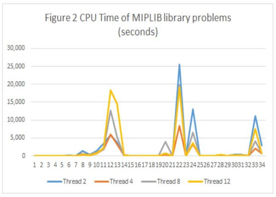
Figure 2. CPU time for MIPLIB library problems.

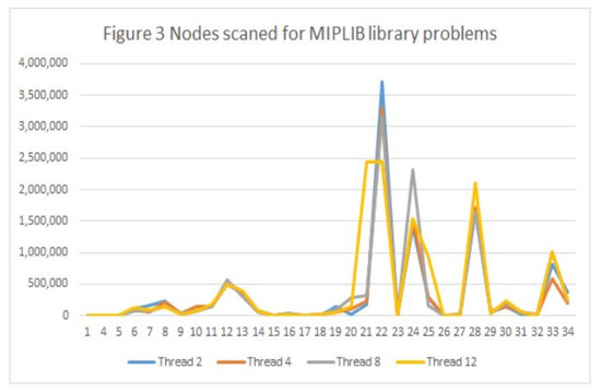
Figure 3. Nodes scanned for MIPLIB library problems.

Table 6 shows the results of the MIPLIB library Model 2 (CPU times), for resolutions with different threads. Taking other experiments with two, four, and eight threads, the correlation values were similar, except for the runs with 12 threads, which showed a value of R = 0.38. Table 6 shows that nodes versus the MIPLIB library with two, four, and eight instances of threads had a statistical F-test value demonstrating statistical significance at a 95% confidence level. The experiment with 12 nodes was significant at a 90% confidence level. All threads show a good fit, with correlation coefficient values ranging from a 0.63 maximum value to a 0.38 minimum. When looking at the explanatory variables’ found values, the x1, x3, and x4 values are similar for all experiments. The ${\lambda }_{min}\left(Q\right)$ found values are similar for all threads. The same is true for all explanatory variables, while the regression coefficients show negative values for all variables. We also observed that all the explanatory variables’ coefficients were negative. This showed an inverse relationship with the $B\&B$ number of nodes. For example, the higher the ${\lambda }_{min}\left(Q\right)$ value, the greater the CPU time, and vice versa. Additionally, we observed that the correlations between different threads’ coefficient values were slightly different. The highest value was 0.63, and the lowest was 0.38. We must note that this last value was seen in the regression with 12 threads, which showed a test value of F = 0.804. This indicates that the experiment was not statistically significant.

Table 6. Model 2 (CPU time) results for resolutions with different threads in MIPLIB library.

Regression Statistics	2 Thread Time	4 Thread Time	8 Thread Time	12 Thread Time
Multiple correlation coefficient	0.58	0.63	0.579	0.38
test F	2.474	3.130	2.355	0.804
Remarks	34	34	34	34
Variable $X_1$ = ${\lambda }_{max}\left(Q\right)$	−1.961 × 10${}^{-7}$	−4.445 × 10${}^{-8}$	−8.248 × 10${}^{-8}$	−1.159 × 10${}^{-7}$
Variable $X_2$ = ${\lambda }_{min}\left(Q\right)$	−0.34	−0.08	−0.15	−0.20
Variable $X_3$ = ${\mu }_{max}$	−1.913 × 10${}^{-9}$	−4.851 × 10${}^{-10}$	−1.137 × 10${}^{-9}$	−1.357 × 10${}^{-9}$
Variable $X_4$ = ${\mu }_{min}$	−1.837 × 10${}^{-8}$	−5.067 × 10${}^{-9}$	−9.012 × 10${}^{-9}$	−1.318 × 10${}^{-8}$
Variable $X_5$ = $h_{max}\left(x^0\right)$	−160.39	−23.83	−59.59	−56.69
Variable $X_6=h_{min}\left(x^0\right)$	−11,127.64	−2828.07	−3790.14	−7251.32

The multiple linear regression model for the best coefficient F according to the data in Table 5 and Table 6 is as follows.

Model 1: Number of nodes = 244,916.2219 − 9.986 × 10${}^{-6}$$x_1$− 18.197 $x_2$ + 1.820 × 10${}^{-6}$$x_3$− 8.746 × 10${}^{-7}$$x_4$ − 10,190.00 $x_5$ + 626,257 $x_6$

Model 2: CPU time = 220,408 + −4.445 × 10${}^{-8}$$x_1$− 0.08 $x_2$− 4.851 × 10${}^{-10}$$x_3$− 5.067 × 10${}^{-9}$$x_4$− 23.83 $x_5$− 2828.07 $x_6$

4.2. OR-Library Problems with MDMKP Problem Results

We solved a set of 30 problems divided into two sets of 15 problems each. We named them $Ct1$ and $Ct2$, respectively. Table 7 shows the number of nodes of each instance of the set $Ct1$ and $Ct2$ for different threads. Table 8 shows the CPU times in seconds for each instance of the set $ct1$ and $Ct2$ for different threads.

Table 7. Nodes vs. different Cplex threads of the multi-demand multi-dimensional knapsack problem (MDMKP OR-Library) set Ct1 and set Ct2 (nodes).

Set	Problem	Cplex 2 Thread	Cplex 4 Thread	Cplex 8 Thread	Cplex 12 Thread
		Nodes 2	Nodes 4	Nodes 8	Nodes 12
Ct1	p1	46	23	31	44
Ct1	p2	13	8	7	23
Ct1	p3	23	14	14	27
Ct1	p4	6	3	2	5
Ct1	p5	35	14	16	20
Ct1	p6	148	51	62	83
Ct1	p7	16	8	9	17
Ct1	p8	81	21	24	44
Ct1	p9	45	25	25	41
Ct1	p10	7	5	4	7
Ct1	p11	6	5	5	9
Ct1	p12	6	4	5	10
Ct1	p13	14	9	12	18
Ct1	p14	10	7	6	225
Ct1	p15	19	13	15	20
Ct2	p1	2165	1315	754	656
Ct2	p2	436	226	182	243
Ct2	p3	35	20	23	11
Ct2	p4	246	107	82	104
Ct2	p5	976	461	427	432
Ct2	p6	5023	2196	2545	5700
Ct2	p7	1368	639	541	440
Ct2	p8	3730	1467	1798	1414
Ct2	p9	6001	2914	9229	20,732
Ct2	p10	2641	827	1660	1522
Ct2	p11	1137	559	453	476
Ct2	p12	407	120	133	145
Ct2	p13	33	18	17	27
Ct2	p14	1130	415	411	445
Ct2	p15	3483	3113	3851	645

Table 8. CPU times vs. different Cplex threads of the multi-demand multi-dimensional knapsack problem (MDMKP OR-Library) sets Ct1 and Ct2 (CPU time in seconds).

Problem	Cplex 2 Thread	Cplex 4 Thread	Cplex 8 Thread	Cplex 12 Thread
	CPU Time 2	CPU Time 4	CPU Time 8	CPU Time 12
Ct1	p1	294,370	370,529	354,355	391,377
Ct1	p2	82,096	105,689	83,213	141,773
Ct1	p3	150,846	166,753	155,003	223,589
Ct1	p4	23,424	28,788	1,385,711	28,982
Ct1	p5	177,854	190,111	176,672	171,314
Ct1	p6	1,060,425	901,951	1,096,551	931,373
Ct1	p7	101,832	101,978	109,418	128,464
Ct1	p8	611,902	317,520	321,045	509,262
Ct1	p9	362,827	422,673	380,613	490,323
Ct1	p10	34,761	49,796	41,538	41,412
Ct1	p11	37,643	53,346	58,842	45,170
Ct1	p12	33,891	40,987	68,945	44,145
Ct1	p13	90,914	107,400	131,613	115,225
Ct1	p14	64,117	74,449	58,948	125,946
Ct1	p15	124,365	163,650	183,902	155,928
Ct2	p1	12,090,448	13,819,244	11,527,542	10,447,674
Ct2	p2	2,909,347	3,608,101	3,045,452	3,623,566
Ct2	p3	2,681,96	330,824	423,069	81,786
Ct2	p4	1,610,790	1,656,464	1,385,711	14,631,259
Ct2	p5	6,097,867	7,033,626	6,156,821	6,904,771
Ct2	p6	18,649,806	18,544,436	18,656,819	18,649,806
Ct2	p7	6,323,089	6,616,805	6,210,114	6,160,737
Ct2	p8	16,071,919	15,531,813	16,578,618	16,089,911
Ct2	p9	25,154,953	23,455,342	24,639,302	28,994,168
Ct2	p10	13,818,283	11,907,287	15,849,302	15,051,050
Ct2	p11	6,560,371	7,598,282	7,379,091	6,779,751
Ct2	p12	1,855,148	1,779,310	2,112,043	1,670,868
Ct2	p13	181,362	218,802	218,258	223,567
Ct2	p14	7,086,563	7,259,420	7,398,144	7,571,377
Ct2	p15	13,782,664	14,672,784	13,406,243	9,236,575

The estimation of Models 1 and 2 was performed with the 30 results obtained from the instances of Ct1 and Ct2. The regression results of Model 1 are shown in Table 9, and the results of Model 2 are shown in Table 10. The first notable result is that the set regression coefficients are values higher than 0.86 for Model 1 and 0.57 for Model 2. This is a medium–high correlation. It can be observed that in Model 1, the values of the correlation coefficient are high and that the F-test shows critical values lower than 1% for all the threads, which indicates that the experiment is statistically significant for all threads. Regarding Model 2, the experiments with two and four threads show critical values lower than 1%, while the results of experiments resolved with 8 and 12 threads present critical values higher than 5%, which makes them less reliable. This is curious since it would be expected that with more threads, the estimate would be more reliable. Finally, the most reliable model estimating the complexity of solving an integer programming model is Model 1, since the explained variable is the number of nodes visited by the $B\&B$, while Model 2 uses the CPU time and this depends on the computer used.

Table 9. Model 1 OR-Library problem results with MDMKP problems. Sets Ct1 and Ct2 (nodes).

Problem	Model 1	Model 1	Model 1	Model 1
	Nodes 2 Thread	Nodes 4 Tthread	Nodes 8 Thread	Nodes 12 Thread
Multiple correlation coefficient	0.7905	0.7860	0.7996	0.8126
Remark	30	30	30	30
Test F	6.38	6.19	6.790	7.45
Critical value of F	0.0004	0.0005	0.0003	0.0001
Intercept	−4.20141 × 10${}^{14}$	−4.63514 × 10${}^{14}$	−3.5531 × 10${}^{14}$	−5.12549 × 10${}^{14}$
Variable $X_1$ = ${\lambda }_{max}\left(Q\right)$	−8365.365	−8091.3780	−8516.669	−12,128.824
Variable $X_2$ = ${\lambda }_{max}\left(Q\right)$	4,476,702.826	8,589,483.231	−1,099,153.01	−2,331,837.54
Variable $X_3$ = ${\lambda }_{min}\left(Q\right)$	0.0428	0,0415	0,0444	0,0530
Variable $X_4$ = ${\mu }_{max}$	2.1007 × 10${}^{14}$	2.31757 × 10${}^{14}$	1.77655 × 10${}^{14}$	2.563 × 10${}^{14}$
Variable $X_5$ = ${\mu }_{min}$	−6563.823	−4033.059	−8197.559	−8861.325
Variable $X_6$ = $h_{max}\left(x^0\right)$	−692,266.948	−2,125,303.665	−200,762.974	303,964.749

Table 10. Model 2 OR-Library problem results with MDMKP problems. Sets Ct1 and Ct2 (CPU time).

Problem	Model 2	Model 2	Model 2	Model 2
	CPU Time 2 Thread	CPU Time 4 Thread	CPU Time 8 Thread	CPU Time 12 Thread
Multiple correlation coefficient	0.762	0.628	0.578	0.591
Remark	30	30	30	30
Test F	5.31	2.50	1.92	2.06
Critical value of F	0.0014	0.05	0.119	0.097
Intercept	−64,363,757,062	−21,401,703,335	−78,486,829,134	−3173 × 10${}^{11}$
Variable $X_1$ = ${\lambda }_{max}\left(Q\right)$	−1.901	−0.204	−1.661	−7.636
Variable $X_2$ = ${\lambda }_{max}\left(Q\right)$	269.798	3365.801	7322.201	3134.783
Variable $X_3$ = ${\lambda }_{min}\left(Q\right)$	9.826 × 10${}^{-6}$	2.690 × 10${}^{-6}$	7.498 × 10${}^{-6}$	2.457 × 10${}^{-5}$
Variable $X_4$ = ${\mu }_{max}$	32,181,877,396	10,700,850,993	39243410216	1.586 × 10${}^{11}$
Variable $X_5$ = ${\mu }_{min}$	−2.0594	−0.0214	−0.3841	−3.0742
Variable $X_6$ = $h_{max}\left(x^0\right)$	411.355	41.793	946.729	1542.990

The multiple linear regression model for the best coefficient F according to the data in Table 9 and Table 10 is as follows.

Model 1: Number of nodes = −3.5531 × 10${}^{14}$− 8516.669 $x_1$ 1,099,153.01 $x_2$ + 0.0444 $x_3$ +1.776 $x_4$ − 8197.559 $x_5$− 200,762.974 $x_6$.

Model 2: CPU time = − 64,363,757,062 + −1.901 $x_1$ + 269.798 $x_2$ + 9.826 × 10${}^{-6}$$x_3$ + 32,181,877,396 $x_4$− 2.0594 $x_5$ + 411.355 $x_6$.

4.3. Estimated Multiple Linear Regression Model Validation

To confirm the developed models, we first calculated the determination coefficient values corresponding to the correlation coefficient square $R^2$. Second, we performed an F-test value analysis of variance and obtained the corresponding critical value

$$R^2=\frac{cov(y,y_1)}{sd\left(y\right)sd\left(y_1\right)}$$

(34)

where y is the observed value and $y_1$. The typically used multiple correlation coefficient is $\rho$ = $\sqrt{R^2}$.

Table 11 summarizes the implemented regression models. Each case shows the regression coefficient and its corresponding F-test value. Table 11 shows that one model only has a linear regression coefficient above 0.5. It is Model 2 (CPU time), solved with 12 treads. Accordingly, the F-test value is low, with a high statistical type I error. Model 1 (nodes) shows linear regression values above 0.5, with nine of them above 0.6. Therefore, we conclude that the used explanatory variables are adequate to explain the $B\&B$ algorithm’s number of nodes and CPU time.

Table 11. Multiple correlation coefficients for problems of MIPLIB library.

Regression Statistics	2 Thread Nodes	4 Thread Nodes	8 Thread Nodes	12 Thread Nodes
Model 1 Miplib
Multiple correlation	0.611	0.602	0.553	0.541
coefficient
test F	2.783	2.662	2.063	1.939
Model 2 Miplib
Multiple correlation	0.58	0.63	0.579	0.38
coefficient
test F	2.474	3.130	2.355	0.804
Model 1 MDMKP
Multiple correlation	0.790	0.786	0.799	0.812
coefficient
Test F	6.38	6.19	6.790	7.45
Model 2 MDMKP
Multiple correlation	0.762	0.628	0.578	0.591
coefficient
Remark	30	30	30	30
Test F	5.31	2.50	1.92	2.06

4.4. Reliability and Generality Level

To estimate the experiments’ reliability and show their generality level, we conducted a reliability analysis, as shown in Table 12. We considered reliability in terms of two values: the multiple linear correlation coefficient Rho and the F-statistic. The former measures the estimate quality determined by the explanatory variables from $x_1$ to $x_6$. The latter measures the performed experiments’ reliability. Both variables complement each other, as the experiments must be reliable and the estimation must have a high correlation. We provide Table 12 to show the Rho and F results. The first block shows the 95% and 90% confidence intervals of the MIPLIB public library problem instances for the Rho coefficient and the ANOVA test F-value. The Rho and F values are random variables, in an experimental sense, as they are the results of conducted experiments. We applied multiple linear regressions between the explained variable nodes and the explanatory variables $x_1$ to $x_6$, and between the explained variable CPU time and the explanatory variables $x_1$ to $x_6$.

Table 12. Reliability of the statistical parameter estimation process.

Database	2 Thread	4 Thread	8 Thread	12 Thread	Media	Standard	95% Confidence	95% Confidence	95% Confidence	90% Confidence	90% Confidence	90% Confidence
MIPLIB	Nodes	Nodes	Nodes	Nodes		Deviation	Interval	Interval	Interval	Interval	Interval	Interval
							Left Limit	Right Limit	Width (%)	Left Limit	Right Limit	Width (%)
Coefficient $\rho$	0.611	0.602	0.553	0.541	0.576	0.0348	0.528	0.625	16.8	0.539	0.613	12.8
Statistic F	2.78	2.66	2.06	1.93	2.36	0.422	1.774	2.949	49.7	1.91	2.81	38.1
Database	2 thread	4 thread	8 thread	12 thread	Media	Standard	95% confidence	95% confidence	95% confidence	90% confidence	90% confidence	90% confidence
MIPLIB	CPU Time	CPU Time	CPU Time	CPU Time		deviation	interval	interval	interval	interval	interval	interval
							left limit	right limit	width (%)	left limit	right limit	width (%)
Coefficient $\rho$	0.58	0.63	0.579	0.38	0.542	0.110	0.388	0.696	56.78	0.424	0.66	43.5
Statistic F	2	3.13	2.355	0.804	2.191	0.985	0.821	3.56	125.032	1.14	3.24	95.79
Database	2 thread	4 thread	8 thread	12 thread	Media	Standard	95% confidence	95% confidence	95% confidence	90% confidence	90% confidence	90% confidence
OR-Library	nodes	nodes	nodes	nodes		deviation	interval	interval	interval	interval	interval	interval
							left limit	right limit	width (%)	left limit	right limit	width (%)
Coefficient $\rho$	0.709	0.786	0.799	0.812	0.776	0.046	0.712	0.841	16.6	0.727	0.826	12.7
Statistic F	6.38	6.19	6.79	7.45	6.70	0.557	5.927	7.487	23.1	6.1	7.29	17.7
Database	2 thread	4 thread	8 thread	12 thread	Media	Standard	95% confidence	95% confidence	95% confidence	90% confidence	90% confidence	90% confidence
OR-Library	CPU Time	CPU Time	CPU Time	CPU Time		deviation	interval	interval	interval	interval	interval	interval
							left limit	right limit	width (%)	left limit	right limit	width (%)
Coefficient $\rho$	0.762	0.628	0.578	0.591	0.639	0.084	0.523	0.757	36.5	0.55	0.729	28.0
Statistic F	5.0	2.5	1.92	2.06	2.94	1.594	0.731	5.164	150.367	1.24	4.64	115.2

We ran a total of 34 instances of the MIPLIB library corresponding to the set covering problem and other similar problem structures, and 30 instances of the OR-Library solving the MDMKP problem. We solved each problem set of 34 and 30 instances using RAM types with different numbers of operating system threads. Each thread generated one result, and these constituted the sample, whose size was 4. As usual, we assumed that the variables Rho and F followed an exponential distribution with unknown mean and variance. Thus, we used Student’s t-distribution to find the critical values needed to construct confidence intervals for the means of both variables, from the MIPLIB and OR-Library instances’ results. The results in Table 12 show that the average value for the Rho correlation coefficient for the explained variable nodes was 0.576 for MKIPLIB instances and 0.7776 for MDMKP instances. Both values show that the number of explanatory variables has a good capacity to estimate the number of nodes visited by the $B\&B$ algorithm.

The 95% confidence interval for Rho in the MIPLIB library instances, when the explained variable is the number of nodes, has a width of 16.8% with respect to the mean. This implies that with 95% probability, the Rho value will be between 0.528 and 0.625. For MDMKP instances, when the explained variable is the number of nodes, the confidence interval width is 16.6% of the mean. These values show that the explanatory variables from $x_1$ to $x_6$ are good predictors for the variable nodes visited by the $B\&B$. The confidence interval indicates that with 95% probability, the Rho values are between 0.712 and 0.841.

The average value for the Rho correlation coefficient, when the explained variable was the CPU time, was 0.542 for MIPLIB instances and 0.639 for MDMKP instances. Both values show a good capability to estimate the CPU time variable. The confidence interval for this variable is 95%, with a width of 23.1% with respect to the mean for MIPLIB instances, and 14.9% with respect to the mean for MDKMKP instances. The 90% confidence interval shows a width of 12.8% with respect to the mean; this is narrower than the previous one and with a lower confidence level. Table 11 shows that the number of visited nodes is an explained variable with a better estimation capacity, which confirms the use of the B&B node tree as a measure of computational effort.

Regarding the F-statistical analysis, Table 12 shows that its variability is low when the explained variable is the number of nodes. The variation coefficient is 0.17 for MIPLIB instances and 0.08 for MDKP instances. When the explained variable is the CPU time, the values of the variation coefficient are 0.44 for MIPLIB and 0.54 for MDMKP instances. This analysis confirms that the number of nodes estimation, using the variables $x_1$ to $x_6$, is highly reliable. The CPU time estimation, with the same variables, is moderately reliable.

5. Discussion

We compared this work’s results with other researchers’ findings. We found that the only comparable published result is that of Hendel et al., published in 2021 [20]. There is a substantive difference from our work. Hendel et al. presented estimation methods that drew on the results of $B\&B$ algorithm execution, whereas our estimators are applicable before the execution of $B\&B$. Hendel et al.’s estimation methods implemented four predictors for the tree size using SCIP integer linear programming software [21]. These predictors estimated the gap between the number of nodes and the unknown final tree during the $B\&B$ algorithm’s execution. The prediction used one explanatory variable only, which was the number of leaves of the tree. A leaf is an end node that no longer branches. The used estimation methods included the tree weight, leaf frequency, Weighted Backtrack Estimator (WBE), and Sum of Subtree Gaps (SSG). Each of them uses a series with double exponential smoothing (DES). They used a level value and a trend value. The software, during the $B\&B$ algorithm’s execution, delivered the models’ data feedings. Hendel et al. [20] applied this to the MIPLIb 2017 library danoint instance. The results showed that the methods were unsuccessful until the execution was partially completed. After this point, the estimation improved, with good results after 80% execution. The prediction methods improved with greater data availability.

Our linear regression method uses geometric variables to estimate the tree size and the CPU time. It is comparable to Hendel et al.’s estimates with few iterations. Our method has 60% reliability given by the coefficient of determination. This % is higher than that of the methods in [20], for estimates up to 66% algorithm execution. In addition, our method to predict the $B\&B$ tree and CPU time to compute the explanatory variables is mathematically simple. It implies calculating Q matrix eigenvalues and other low-complexity calculations. Therefore, these complexity measures can be embedded into available software to predict the resolution time a priori. This is a topic that has great practical importance for available software efficiency. However, few researchers have examined the area, and there is a restricted volume of scientific production. We found no more than 10 publications, and most are outdated.

Finally, this study has some limitations. The first is that the results are valid for the data obtained with the tested problems. This is a limited sample that allows us to see a trend. It is not generalizable to a larger context, without the risk of extrapolation errors. Another limitation is that, for some problems, obtaining the analytical solution presents computational complications. This is because solutions are obtained via a nonlinear method, a Newton-type method. For many problems, our algorithm to obtain the analytical center took longer than ten hours to deliver a solution. The 10-h limitation is important because this study provides problem complexity indicators, and if the analytical center calculation takes a long time, it is no longer feasible to use it for these purposes.

6. Conclusions

In this work, we investigated integer programming based on the flatness theorem and conditioning in integer programming. It was a theoretical and applied work. We developed the measures and then implemented and tested them as $B\&B$ tree predictors. Within the integer programming context, we developed geometric measurements to estimate the CPU time and number of nodes visited by the $B\&B$ algorithm, based on the concept of conditioning in integer programming. The results showed high values for multiple correlation coefficients. The used explanatory variables came from one of the dimensions proposed for the width of the relaxed polyhedron ellipsoid constructed with the problem’s constraints. The explanatory variables correspond to expressions associated with a Dikin ellipse matrix within the polyhedron that replicates the shape of the polyhedron. Here, the analytical center was the analytical polyhedron center. One limitation of this work is the analytical center calculation. This is because solving a nonlinear problem requires a large amount of CPU time. In some problems, results exceed the ten-hour limit. The calculation of the center of the polyhedron is typical of the interior point methods for linear programming, such as the Karmakar algorithm and the ellipsoidal method, which use analysis techniques and nonlinear programming methodology. However, this is a bottleneck when we wish to obtain $B\&B$ effort estimation measures that need to be calculated quickly. Thus, one line of future work is to study how to speed up the calculation of these indices, so that they can be incorporated into linear optimization software. To achieve this, other centers of the polyhedron can be explored, such as the center developed by the method of the central path. This can be used directly as a feasible center of the Dikin ellipse, or it can be used to approximate the analytic center, under certain conditions. Its solution no longer requires solving a nonlinear problem, but a classic simplex.

References

- Karp, R.M. Complexity of computer computation. In Reducibility among Combinatorial Problems; Springer: Berlin/Heidelberg, Germany, 1972; pp. 85–103. [Google Scholar]
- Skiena, S. The Algorithm Design Manual; Springer: New York, NY, USA, 1997; pp. 32–58. [Google Scholar]
- Crescenzi, P.; Kann, V.; Halldórsson, M.; Karpinski, M.; Woeginger, G. A compendium of NP optimization problems. Braz. J. Oper. Prod. Manag. Available online: http://www.nada.kth.se/~viggo/problemlist/compendium.html (accessed on 12 June 2023).
- Garey, M.; Johnson, D. Computers and Intractability: A Guide to the Theory of NP-Completeness; W.H. Freeman: New York, NY, USA, 1979. [Google Scholar]
- Fréville, A. The multidimensional 0–1 knapsack problem: An overview. Eur. J. Oper. Res. 2004, 155, 1–21. [Google Scholar] [CrossRef]
- Derpich, I.; Herrera, C.; Sepulveda, F.; Ubilla, H. Complexity indices for the multidimensional knapsack problem. Cent. Eur. J. Oper. Res. 2021, 29, 589–609. [Google Scholar] [CrossRef]
- Knuth, D. Estimating the efficiency of backtrack programs. Math. Comput. 1975, 29, 122–136. [Google Scholar] [CrossRef]
- Purdom, P.W. Tree size by partial backtracking. SIAM J. Comput. 1978, 7, 481–491. [Google Scholar] [CrossRef]
- Chen, P.C. Heuristic sampling: A method for predicting the performance of tree searching programs. SIAM J. Comput. 1992, 21, 295–315. [Google Scholar] [CrossRef]
- Belov, G.; Esler, S.; Fernando, D.; Le Bodic, P.; Nemhauser, G.L. Estimating the Size of Search Trees by Sampling with Domain Knowledge. In Proceedings of the Twenty-Sixth International Joint Conference on Artificial Intelligence (IJCAI-17), Melbourne, Australia, 19–25 August 2017; pp. 473–479. [Google Scholar]
- Pierre Le Bodic, P.; Nemhauser, G.L. An Abstract Model for Branching and its Application to Mixed Integer Programming. Math. Program. 2015, 166, 369–405. [Google Scholar] [CrossRef]
- Lelis, L.H.; Otten, L.; Dechter, R. Predicting the size of depth-first branch and bound search trees. In Proceedings of the Twenty-Third International Joint Conference on Artificial Intelligence, Beijing, China, 3–9 August 2013; pp. 594–600. [Google Scholar]
- Ozaltın, Y.; Hunsaker, B.; Schaefer, A.J. Predicting the solution time of branch-andbound algorithms for mixed-integer programs. INFORMS J. Comput. 2011, 23, 392–403. [Google Scholar] [CrossRef]
- Alvarez, M.; Louveaux, Q.; Wehenkel, L. A Supervised Machine Learning Approach to Variable Branching in Branch-and-Bound. Technical Report, Universite de Liege. 2014. Available online: https://orbi.uliege.be/handle/2268/167559 (accessed on 12 June 2023).
- Benda, F.; Braune, R.; Doerner, K.F.; Hartl, R.F. A machine learning approach for flow shop scheduling problems with alternative resources, sequence-dependent setup times, and blocking. OR Spectr. 2019, 41, 871–893. [Google Scholar] [CrossRef]
- Lin, J.C.; Zhu, J.L.; Wang, H.G.; Zhang, T. Learning to branch with Tree-aware Branching Transformers. Knowl.-Based Syst. 2022, 252, 109455. [Google Scholar] [CrossRef]
- Kilby, P.; Slaney, J.; Sylvie Thiebaux, S.; Walsh, T. Estimating Search Tree Size. In Proceedings of the Twenty-First National Conference on Artificial Intelligence and the Eighteenth Innovative Applications of Artificial Intelligence Conference, Boston, MA, USA, 16–20 July 2006; pp. 1–7. [Google Scholar]
- Fischetti, M.; Monaci, M. Exploiting Erraticism in Search. Oper. Res. 2014, 62, 114–122. [Google Scholar] [CrossRef]
- Hendel, G.; Anderson, D.; Le Bodic, P.; Pfetschd, M.E. Estimating the Size of Branch-and-Bound Trees. INFORMS J. Comput. 2021, 34, 934–952. [Google Scholar] [CrossRef]
- Bestuzheva, K.; Besançon, M.; Wei-Kun, C.; Chmiela, A.; Donkiewicz, T.; van Doornmalen, J.; Eifler, L.; Gaul, O.; Gamrath, G.; Gleixner, A.; et al. The SCIP Optimization Suite 8.0. 2021. Available online: https://optimization-online.org/2021/12/8728/ (accessed on 12 June 2023).
- Renegar, J.; Belloni, A.; Freund, R.M. A geometric analysis of Renegar’s condition number, and its interplay with conic curvature. Math. Program. 2007, 119, 95–107. [Google Scholar]
- Vera, J. On the complexity of linear programming under finite precision arithmetic. Math. Program. 1998, 80, 91–123. [Google Scholar] [CrossRef]
- Cai, Z.; Freund, R.M. On two measures of problem instance complexity and their correlation with the performance of SeDuMi on second-order cone problems. Comput. Optim. Appl. 2006, 34, 299–319. [Google Scholar] [CrossRef]
- Vera, J.; Derpich, I. Incorporando condition measures in the context of combinatorial optimization. SIAM J. Optim. 2006, 16, 965–985. [Google Scholar] [CrossRef]
- Lenstra, H.W., Jr. Integer programming with a fixed number of variables. Math. Oper. Res. 1983, 8, 538–548. [Google Scholar] [CrossRef]
- Koch, T.; Achterberg, T.; Andersen, E.; Bastert, O.; Berthold, T.; Bixby, R.E.; Danna, E.; Gamrath, G.; Gleixner, A.M.; Heinz, S.; et al. MIPLIB 2010: Mixed Integer Programming Library version 5. Math. Prog. Comp. 2011, 3, 103–163. [Google Scholar] [CrossRef]
- Gleixner, A.; Hendel, G.; Gamrath, G.; Achterberg, T.; Bastubbe, M.; Berthold, T.; Christophel, P.; Jarck, K.; Koch, T.; Linderoth, J.; et al. Miplib 2017: Data-Driven Compilation of the 6th Mixed-Integer Programming Library. Math. Program. Comput. 2017, 13, 443–490. [Google Scholar] [CrossRef]
- Beasley, J.E. OR-Library: Distributing test problems by electronic mail. J. Oper. Res. Soc. 1990, 41, 1069–1072. [Google Scholar] [CrossRef]
- Khintcine, A. A quantitative formulation of Kronecker’theory pf approximation. Izv. Ross. Akad. Nauk. Seriya Mat. 1948, 12, 113–122. (In Russian) [Google Scholar]
- Freund, R.M.; Vera, J.R. Some characterizations and properties of the “distance to ill-posedness” and the condition measure of a conic linear system. Math. Program. 1999, 86, 225–260. [Google Scholar] [CrossRef]
- Jhon, F. Extremum problems with inequalities as subsidiary conditions. In Studies and Essays; Intersciences: New York, NY, USA, 1948; pp. 187–204. [Google Scholar]
- Schrijver, A. Chapter 14: The ellipsoid method for polyhedra more generally. In Theory of Linear and Integer Programming; Wiley Interscience Series; John Wiley & Sons: Hoboken, NJ, USA, 1986; pp. 172–189. [Google Scholar]
- Nesterov, Y.; Nemirosky, A. Acceleration and parallelization of the path-following interior point method for a linearly constrainde convex quadratic problem. Siam J. Optim. 1991, 1, 548–564. [Google Scholar] [CrossRef]
- Elhedhli, S.; Naom-Sawaya, J. Improved branching disjunctions for branch-and-bound: An analytic center approach. Eur. J. Oper. Res. 2015, 247, 37–45. [Google Scholar] [CrossRef]
- Micciancio, D. The shortest vector in a lattice is hard to approximate to within some constants. SIAM J. Comput. 2001, 30, 2008–2035. [Google Scholar] [CrossRef]
- Vazirani, V. Approximation Algorithms; Springer-Verlag: Berlin, Germany, 2001; ISBN 3-540-65367-8. [Google Scholar]
Disclaimer/Publisher’s Note: The statements, opinions and data contained in all publications are solely those of the individual author(s) and contributor(s) and not of MDPI and/or the editor(s). MDPI and/or the editor(s) disclaim responsibility for any injury to people or property resulting from any ideas, methods, instructions or products referred to in the content. |
© 2023 by the authors. Licensee MDPI, Basel, Switzerland. This article is an open access article distributed under the terms and conditions of the Creative Commons Attribution (CC BY) license (https://creativecommons.org/licenses/by/4.0/).