Abstract
Higher accuracy in cluster failure prediction can ensure the long-term stable operation of cluster systems and effectively alleviate energy losses caused by system failures. Previous works have mostly employed BP neural networks (BPNNs) to predict system faults, but this approach suffers from reduced prediction accuracy due to the inappropriate initialization of weights and thresholds. To address these issues, this paper proposes an improved arithmetic optimization algorithm (AOA) to optimize the initial weights and thresholds in BPNNs. Specifically, we first introduced an improved AOA via multi-subpopulation and comprehensive learning strategies, called MCLAOA. This approach employed multi-subpopulations to effectively alleviate the poor global exploration performance caused by a single elite, and the comprehensive learning strategy enhanced the exploitation performance via information exchange among individuals. More importantly, a nonlinear strategy with a tangent function was designed to ensure a smooth balance and transition between exploration and exploitation. Secondly, the proposed MCLAOA was utilized to optimize the initial weights and thresholds of BPNNs in cluster fault prediction, which could enhance the accuracy of fault prediction models. Finally, the experimental results for 23 benchmark functions, CEC2020 benchmark problems, and two engineering examples demonstrated that the proposed MCLAOA outperformed other swarm intelligence algorithms. For the 23 benchmark functions, it improved the optimal solutions in 16 functions compared to the basic AOA. The proposed fault prediction model achieved comparable performance to other swarm-intelligence-based BPNN models. Compared to basic BPNNs and AOA-BPNNs, the MCLAOA-BPNN showed improvements of 2.0538 and 0.8762 in terms of mean absolute percentage error, respectively.
Keywords:
arithmetic optimization algorithm; multi-subpopulation; comprehensive learning; BP neural network; failure prediction MSC:
68T20; 90C26
1. Introduction
In recent years, due to the rapid development of computer technology, computer systems have been widely applied in various industries within the national economy, greatly promoting socioeconomic development. At the same time, higher requirements have been placed on the sustainable and stable operation of computer systems, and people are increasingly concerned about the availability of computer systems [1,2,3,4,5]. Currently, providing continuous and stable services in control cluster systems is an urgent issue in computer cluster technology.
Previous work has mostly focused on load balancing [6,7], resource scheduling [4,8], fault tolerance [9,10], and other aspects of cluster systems. However, recently, limited research has been conducted on improving system stability through fault prediction. Control cluster fault prediction aims to predict node failures at an early stage, enabling proactive resource scheduling and enhancing the availability of the cluster system. Pinto et al. [11] designed a distributed computing system for Hadoop clusters and used SVM for cluster fault prediction. Mukwevho et al. [12] analyzed three fault-tolerant techniques and achieved fault prediction through proactive methods. Das et al. [13] employed log analysis for fault prediction. However, most of these fault prediction approaches required building custom models according to specific requirements and were not widely applicable, and while neural-network-based fault prediction can be widely applied, it suffers from issues such as slow convergence and susceptibility to local optima due to sensitivity to initial weights and thresholds. Fortunately, swarm intelligence approaches can effectively adjust these parameters. The novel research field successfully combines machine learning and swarm intelligence approaches and proved to be able to obtain outstanding results in different areas [14,15]. Therefore, in this work, we design a novel intelligent algorithm and employ it to find the optimal parameters in the neural network prediction model.
The arithmetic optimization algorithm (AOA) is a new metaheuristic algorithm proposed by Abualigah et al. in 2021, which primarily utilizes basic arithmetic operators to perform exploration (multiplication and division) and exploitation (subtraction and addition) [16]. The algorithm’s main advantages lie in its simplicity, ease of programming, and fewer parameters [17], which have led researchers to apply it in various fields, including engineering design [18,19,20], cloud computing [21], and image processing [22], to name a few [23,24,25]. However, the AOA faces challenges in dealing with complex optimization problems, particularly regarding issues of local optima and slow convergence. Recently, improved versions of the AOA have emerged as a trend. For example, Li et al. [18] employed 10 chaotic maps to modify the control parameters and improve the exploration and exploitation stages during the iteration process. However, this approach did not modify the mathematical model, which implies that it may still encounter local optima when faced with complex optimization problems. Çelik [19] employed information exchange [26,27], Gaussian distribution [26], and quasi-opposition [28,29] to propose an information-exchanged Gaussian AOA with quasi-opposition learning (IEGQO-AOA), which improved the convergence performance without significantly increasing the computational complexity of the algorithm. Gölcük et al. [23] employed highly disruptive polynomial mutation and local escaping operators to propose an improved AOA for training feedforward neural networks. These methods [19,23] employed mutation factors to improve the exploration performance of the AOA, enabling it to escape local optima. However, mutation factors may generate solutions that deviate from the optimal solution, thus reducing the convergence speed. Kaveh et al. [25] improved population diversity and convergence performance by modifying the mathematical model in the exploration and exploitation stage of the AOA and applied the improved AOA to structural optimization. Some research works have improved the performance of the AOA by combining it with other meta-heuristic algorithms, such as the sine cosine algorithm (SCA) [20], the salp swarm algorithm (SSA) [21], and the aquila optimizer (AO) [30]. It is worth noting that the aforementioned algorithms improved the global optimization performance by introducing mutation factors, modifying the control parameters, or incorporating other algorithms.
Swarm intelligence algorithms consist of two main phases, namely exploration and exploitation [31,32,33,34]. The purpose of exploration is to search the regions where the global optimum may exist. Exploitation aims to further refine and precisely search the promising regions identified during exploration. It is well known that the key to optimizing performance in swarm intelligence lies in the search capabilities of exploration and exploitation, as well as the balance and transition between these two phases. However, the AOA utilizes multiplication and division operators in the exploration phase and addition and subtraction operators in the exploitation phase, and it revolves around a single elite individual without involving information sharing among individuals. These limitations greatly restrict the exploration and exploitation performance of the algorithm. In addition, a linear mechanism does not accurately reflect the complex optimization process; therefore, it fails to facilitate a smooth transition from the exploration phase to the exploitation phase.
Motivated by the aforementioned analysis, we proposed a novel improved AOA via multi-subpopulation (MS) and comprehensive learning (CL) strategies for global optimization (MCLAOA). Subsequently, the MCLAOA was combined with a BP neural network (BPNN) to form the MCLAOA-BPNN model for cluster fault prediction. Firstly, we proposed the novel MCLAOA. Specifically, the MS was applied in the exploration phase, where we divided the population into several subpopulations, and each subpopulation revolved around its own sub-elite. This strategy alleviated the weakness of a single elite in terms of exploration performance and enhanced population diversity. The CL was used in the exploitation phase to increase the information sharing among individuals and sped up the convergence of the algorithm. In addition, to ensure a smooth transition from the exploration phase to the exploitation phase, a nonlinear math optimizer accelerated (MOA) with a tangent function was employed instead of the standard MOA. After obtaining the high-performance MCLAOA, we combined it with the BPNN to form the MCLAOA-BPNN cluster fault prediction model. The model utilized MCLAOA to obtain the best initial weights and thresholds for BPNN, thereby improving prediction accuracy and providing the foundation for resource scheduling and sustainable operation of cluster systems.
In this work, the main contributions are summarized as follows:
- (1)
- To enhance the accuracy of cluster fault prediction, we attempted to design a new optimization algorithm and combined it with BPNN to form the MCLAOA-BPNN cluster fault prediction model. The model utilized MCLAOA to optimize the initial weights and thresholds of BPNN.
- (2)
- To address the lack of individual information sharing in both the exploration and exploitation phases, we proposed the MCLAOA. This approach employed the MS and CL strategies to modify the mathematical models of the exploration and exploitation phases, thereby improving the optimization performance.
- (3)
- To ensure a smooth transition from the exploration phase to the exploitation phase for the MCLAOA, we designed a nonlinear MOA with tangent functions to replace the linear mechanism in the standard AOA.
- (4)
- Experimental results over 23 benchmark functions, CEC2020 benchmark problems, and two engineering examples showed that the proposed MCLAOA has much stronger merit. In addition, the MCLAOA-BPNN had better prediction accuracy compared to other algorithms.
The remainder of this paper is structured as follows: The standard AOA is introduced in Section 2, and the proposed MCLAOA is presented in Section 3. In Section 4, results and analysis of the proposed algorithm are presented using 23 benchmark functions, CEC2020 benchmark problems, and two engineering design problems. Section 5 presents the MCLAOA-BPNN model for cluster fault prediction and compares it with other models. At last, the conclusion of this paper is provided in Section 6.
2. Arithmetic Optimization Algorithm (AOA)
Inspired by the arithmetic operators, the AOA is proposed as a new intelligent algorithm. The basic principle of AOA is shown in Figure 1, which is mainly divided into the exploration phase and the exploitation phase [16].
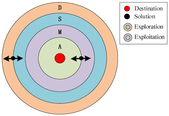
Figure 1.
Updating toward or away from destination.
2.1. Math Optimizer Accelerated (MOA)
Before optimization, the is designed to determine whether the population is performing the exploration phase or the exploitation phase. Here, given a random number between 0 and 1, the global exploration phase is executed if , otherwise, the local exploitation phase is executed. The MOA can be formulated as:
where t and T are the current iteration and the maximum number of iterations, respectively. and represent the maximum value and minimum value of the accelerated function.
2.2. Exploration Phase
In this phase, the AOA mainly adopts division and multiplication search strategy to find better candidate solutions, and the mathematical model is as follows:
where represents the position of the dimension of the individual, and is the dimension in the best solution of all individuals. ∂ is a small integer number that prevents the denominator from being 0. is a parameter representing the step size factor of the current iteration, denotes the step size of the dimension, and is a random number in [0,1]. and represent the upper and lower bound value of the dimension, respectively. is the control parameter that regulates the search process, and is a sensitive parameter. and are set to 0.5 and 5, respectively, according to the literature [16].
2.3. Exploitation Phase
This phase performs the local exploitation. Additive and subtractive operators are adopted to search for the optimal solution. Specifically, given a random number between 0 and 1, if , the subtractive operator is employed to search for the optimal solution, otherwise, the additive operator is employed to update the population position, which can be expressed as follows:
3. Proposed Method
From the mathematical model of AOA, it can be seen that all individuals perform expansion or reduction operations around the elite () in the exploration phase, which affects the search ability of the AOA. The exploitation phase employs a fixed step factor () without memory retention, which can lead to a lack of information exchange between individuals and reduce convergence effectiveness. In addition, the MOA with a linear mechanism cannot solve complex optimization problems. To deal with the above shortcomings, an improved AOA was proposed to solve the global optimization problem by MS strategy and CL strategy. Compared with the standard AOA, three operators, MS, CL and nonlinear MOA with tangent function, were introduced in this paper. The specific mathematical model is as follows.
3.1. Multi-Subpopulation (MS) Strategy
Global search refers to identifying the optimal region for the target within a larger search space to prevent the algorithm from getting trapped in local optima [35,36]. However, according to Equation (2), it is known that all individuals explore the search space based on the and a fixed step size factor (), which reduces population diversity and exploration performance. Therefore, we propose the MS strategy to improve the exploration performance of AOA, as shown in Figure 2.
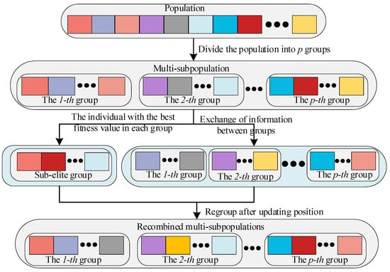
Figure 2.
The flowchart of the MS strategy.
To be specific, first a population size is given, which is divided into p subpopulations. Second, all individuals are evaluated for fitness, and the individual with the minimum fitness value in each group is selected as the sub-elite, forming a sub-elite group. Then, all individuals except for the sub-elite group are rearranged into p groups to explore the search space. Finally, each sub-elite is randomly assigned to different groups. Here, the sub-elite group can be expressed as Equation (6),
where p is the number of sub-elite groups, q represents the number of individuals contained in each sub-population, denotes the inverse function of fitness evaluation, and represents the position of the sub-elite individual in the sub-elite group. By introducing the MS strategy, the diversity of the population can be ensured, the exploration ability can be increased in the search space, and the algorithm can be prevented from falling into local optima.
3.2. Comprehensive Learning (CL) Strategy
After finding some promising solutions during the exploration phase, local exploitation means attempting to delve deeper into these solutions to find better ones [35,36]. However, according to Equations (4) and (5), it can be seen that the position update rule during the exploration phase involves upper and lower bounds without any information exchange between individuals. That is, all individuals only affect the convergence rate by increasing or decreasing a fixed step factor. Inspired by the CL particle swarm optimizer (CLPSO) [37], the CL strategy is used during the exploitation phase. On the one hand, the CL strategy can preserve individual historical information and facilitate information sharing. On the other hand, the population does not learn from all dimensions of a single individual, but rather from different dimensions of the entire population. The learning probability for each dimension is determined based on a probability value [37]. The learning probability for the individual can be described as follows:
where is population size. The pseudo-code of the MCLAOA is shown in Algorithm 1.
| Algorithm 1 Pseudo-code of the CL strategy |
|
1: for i = 1: 2: Generate random number r 3: Compute the learning probability value () using Equation (7). 4: Give the index of two random individuals, and . 5: if 6: if 7: 8: Else 9: 10: End if 11: Else 12: 13: End if 14: End for |
3.3. Improved AOA with MS and CL (MCLAOA)
Based on the above analysis, the MS and CL strategies were introduced into the standard AOA to increase population diversity and improve the convergence performance. For the the MCLAOA, the MS strategy was only applied in the exploration phase, while the CL strategy was only applied in the exploitation phase. The specific details of these improvements will be introduced in the following subsection.
Exploration phase: In this phase, considering that expanding or shrinking by a certain proportion always limits the exploration performance of AOA, inspired by the teaching-learning-based optimization (TLBO) [38], we introduced the teaching phase of TLBO. Specifically, half of the subpopulations adopted the exploration phase of AOA, and the rest adopted the teaching phase.
For the first half of the subpopulation specifically, the MS strategy was introduced in Section 3.1. We employed multiple sub-elites to replace a single elite, increasing the diversity of solutions generated and preventing premature convergence due to local optima issues. We applied Equation (6) to Equation (2), and the modified Equation (2) can be described as:
where represents the position of the dimension of the individual in the group.
For the second half of the population,
where is the average value of all individuals, and denotes the teacher factor ().
Exploitation phase: The standard AOA cannot retain memory during the exploitation phase, which lead to slow convergence. The CL strategy was introduced into Equation (5), individuals can exchange information, speeding up the algorithm’s convergence to the global optimum. Therefore, the specific modification is shown in Equation (10):
where defines the value of the individual in the dimension, which determines whether the individual learns in its own or other individuals’ different dimensions. For choosing its own or other individual’s dimension, it depends on the learning probability in Equation (7). If the random number r is greater than , it is learned from its own dimension , otherwise it occurs from another individual’s dimension .
Modified MOA: The parameter , which varies linearly with the number of iterations, cannot reflect the real optimization problem. Therefore, this paper modifies MOA using non-linear parameters with a tangent function, as shown in Figure 3. The tangent function is introduced into Equation (1), and its modified can be expressed as:
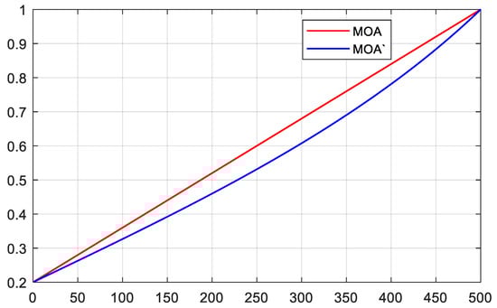
Figure 3.
The MOA with the increase of iterations.
As can be seen from Figure 3, compared with the original , can better balance and transition the exploration and exploitation.
In summary, the MS and teaching strategies were applied in the exploration phase. The MS improved population diversity and enabled faster global search. Furthermore, the search method in the exploration phase is limited by a step factor determined by the upper and lower bounds, which constrains the algorithm’s search capability. Therefore, we introduced the teaching phase of TLBO [38], where collective information from all individuals was used to mitigate this limitation. The CL strategy was applied in the exploitation phase of the algorithm, accelerating the convergence to the global optimum through information exchange among individuals. This strategy addressed the slow convergence issue caused by the addition and subtraction operators. In addition, we designed Equation (11) to effectively balance and smoothly transition between exploration and exploitation. We denote the improved AOA as MCLAOA. The detailed flowchart of the proposed MCLAOA is described in Figure 4. For clarity, the main contributions of this paper are highlighted, including , the exploration phase, and the exploitation phase. In addition, the pseudo-code of MCLAOA is shown in Algorithm 2.
| Algorithm 2 Pseudo-code of the proposed MCLAOA |
|
1: Initialize: population size , position , parameters and , the maximum number of iterations T, p group (sub-population). 2: Update: 3: While 4: Calculate the Fitness Function for the given solutions. 5: Find the best solution (Determined best so far). 6: Update the MOA’ value and MOP value using Equations (11) and (3). 7: for i = 1: 8: for j = 1 to Positions do 9: Generate a random value between [0, 1] (, , and ) 10: if then 11: %%%Exploration phase%%% 12: For the first half of the subpopulation, 13: if then 14: (1) Apply the Division math operator (D “÷”) 15: Update the solutions’ positions using the first rule in Equation (8). 16: Else 17: (2) Apply the Division math operator (M “ ×”) 18: Update the solutions’ positions using the first rule in Equation (8). 19: End if 20: For the second half of the subpopulation, 21: Update the solutions’ positions using Equation (9). 22: Else 23: %%%Exploitation phase%%% 24: Generate random number r 25: Compute the learning probability value () using Equation (7). 26: Decide whether is its own or another individual. 27: if then 28: (1) Apply the Subtraction math operator (S “-”). 29: Update the solutions’ positions using the first rule in Equation (10). 30: Else 31: (2) Apply the Addition math operator (A “+”). 32: Update the solutions’ positions using the second rule in Equation (10). 33: End if 34: End if 35: End for j 36: End for i 37: 38: End While 39: Output: Return the best solution . |
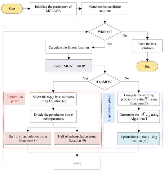
Figure 4.
Flowchart of the proposed MCLAOA.
3.4. Computational Complexity
Compared to the standard AOA, the proposed MCLAOA mainly introduces the MS strategy, CL strategy, and the modified MOA. Considering that the MS strategy involves sub-elite groups, it is necessary to conduct a fitness evaluation ranking, denoted as . The computational complexity of the CL strategy is , where D is the dimension. The computational complexity of the modified MOA is almost unchanged compared to the original MOA. Therefore, the computational complexity of the proposed MCLAOA is . If T is much greater than 1, then .
4. Results and Analysis
The experiments were conducted using MATLAB2017b, and they were run on a PC with Intel Core i7-10700 2.90GHz and 16GB RAM. To examine the performance of the proposed MCLAOA, the 23 benchmark functions and 2 engineering design problems were employed. Among them, 23 benchmark functions [16] are shown in Table 1.

Table 1.
23 benchmark functions.
To verify the advanced performance of the proposed MCLAOA, comparisons were made with several algorithms, including (1) some versions of AOA, such as the AOA [16], the chaotic AOA (CAOA) [18], (2) advanced metaheuristic algorithms, such as the reptile search algorithm (RSA) [39], the whale optimization algorithm (WOA) [40], and the grasshopper optimization algorithm (GOA) [41], (3) the classical metaheuristic algorithm and particle swarm optimization (PSO) [42], and (4) the winner of CEC competition, the L-SHADE [43]. For some versions of AOA, the AOA was employed to validate the effectiveness of MCLAOA, while the CAOA was employed to test the strong competitiveness of MCLAOA compared to the versions of AOA. It is worth noting that the CAOA [18] has been proven to outperform some advanced algorithms, including the HHO [44], the EO [45], and the WHO [46], in certain optimization problems. For advanced and classical metaheuristic algorithms, these comparative algorithms can confirm that the MCLAOA achieves state-of-the-art performance and outperforms classical algorithms of the same type. For the winner of CEC competition, once it is confirmed that the MCLAOA outperforms the LSHADE, it can be classified as a high-performance optimizer. All algorithms were set with parameters as shown in Table 2. For the sake of fairness in comparison, the maximum function evaluation with a population size of and 100,000 was selected for 23 benchmark functions. All algorithms were independently run 30 times on each test function. To compare the superiority and inferiority of these algorithms, the evaluation indicators used were the average () and standard deviation () as well as the best optimal value (), and convergence curves were used to indicate the convergence performance of the algorithms. Box plots were adopted to verify the stability of the algorithms. The Wilcoxon rank-sum test and Friedman rank test were employed to reflect the statistical significance of the algorithms [47]. Next, experimental analysis was conducted on 23 benchmark functions.
Table 2.
The parameter setting of the algorithms.
4.1. Results Comparisons Using 23 Benchmark Functions
The 23 benchmark functions [16] are a classic function benchmark for evaluating optimization algorithms which can be divided into three types: unimodal functions (–), multimodal functions (–), and fixed-dimension multimodal functions (–). For details on the 23 benchmark functions, please refer to Table 1. The experimental results of all algorithms with , , and are shown in Table 3, and the best results of each function are marked in bold type.
Table 3.
Numerical results of MCLAOA with other algorithms using 23 benchmark functions.
4.1.1. Unimodal Functions and Exploitation
The unimodal functions (–) have only one global solution and no local solution, which is used to test the exploitation ability of the algorithm. It can be seen from Table 3 that the proposed MCLAOA has stronger advantages in terms of value compared to other comparison algorithms, except for and . For –, both the MCLAOA and the CAOA achieve convergence with an value of 0, while the RSA also converges to 0. However, the AOA fails to converge to 0 in terms of the metric. These results indicate that the exploitation performance of MCLAOA has been significantly improved. This is attributed to the introduction of the CL strategy which modifies the mathematical model of the exploitation phase and enhances the convergence to the optimal solution by sharing information among individuals.
4.1.2. Multimodal Functions and Exploration
The multimodal function contains multiple local optimal solutions, which are used to test the algorithm’s ability to escape from poor local optima and obtain the near-global optimum. For multimodal functions (–) with a dimension of 30, the value of the proposed MCLAOA ranks first except for and . Compared with high-dimension multimodal functions (–), fixed-dimension multimodal functions (–) have only a few local minima, and the dimension of the function is small and fixed. It is worth noting that the values of all algorithms converge to the global optimum for –, and for –, all algorithms except RSA also converge to the global optimum. These results demonstrate their ability to converge to the global optimum. However, when considering and values together, the proposed MCLAOA exhibits superior performance, indicating its ability to converge more stably to the global optimum. Therefore, it can be seen from the experimental results of multimodal functions that the proposed MCLAOA has good global exploration performance. The MS strategy divides the population into p subpopulations by introducing p sub-elites instead of a single elite. This strategy enhances the global search capability. Additionally, we introduce a teaching phase to half of the subpopulations, which alleviates the limitations of expansion or shrinkage step size factor in the exploration phase of AOA. As a result, the proposed MCLAOA outperforms other algorithms, especially in , –.
4.1.3. Convergence Behavior Analysis
To observe the convergence of the proposed MCLAOA and comparison algorithms, we record and save the fitness of the best solution for each iteration to draw the convergence curve. The convergence results of all algorithms on 23 benchmark functions are shown in Figure 5. It can be seen from Figure 5 that only the CAOA, the RSA, and the MCLAOA show a clear downward trend on –, and the proposed MCLAOA shows a more obvious decrease for and compared to the CAOA and the RSA. For multimodal functions –, the proposed MCLAOA achieves a significantly faster convergence to the global optimum compared to the other seven comparison algorithms. All algorithms can converge to the global optimum for and , but the convergence curve of the proposed MCLAOA drops faster than the AOA and the CAOA. Moreover, the proposed MCLAOA ranks first in convergence performance on – among all comparison algorithms, indicating its good exploitation performance. In summary, the proposed MCLAOA has achieved advanced performance. Compared with the basic AOA and the improved version CAOA, the proposed MCLAOA has improved convergence performance. In addition, since the comparison algorithms are meta-heuristic algorithms with randomness, in this paper, we employ Box plots to analyze the stability of the results. Box plots of the result of a global minimum of the MCLAOA, the AOA, the CAOA, the RSA, the WOA, the GOA, the PSO and the L-SHADE for , , , and are shown in Figure 6. It can be observed from Figure 6 that the proposed MCLAOA outperforms other algorithms in the stability of the results during the running of the algorithm.
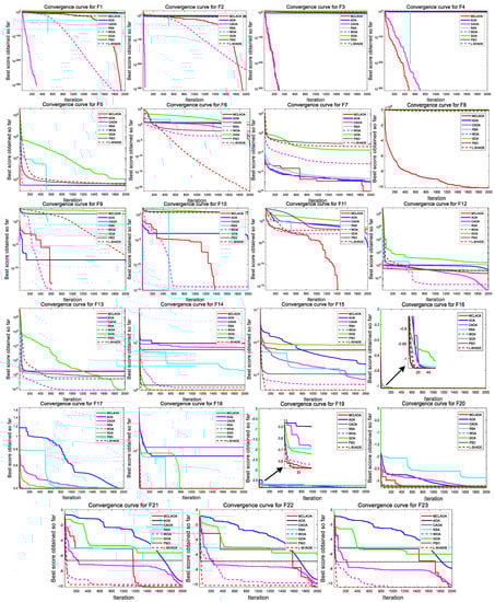
Figure 5.
Convergence curves for 23 benchmark functions. Better viewed in color with zoom-in.
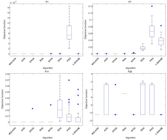
Figure 6.
Box plots of the result of a global minimum for functions , , , and .
Based on the above analysis, the proposed MCLAOA shows strong advantages in terms of convergence accuracy, convergence speed and robustness.
4.2. Statistical Analysis
It is worth mentioning that statistical analysis is very important for the statistical authenticity of results in the field of optimization algorithms. In this paper, the Wilcoxon rank-sum test and the Friedman test are employed.
The statistical results of 23 benchmark functions are shown in Table 4. From the data results in Table 4, it can be observed that the proposed MCLAOA performs better than other comparison algorithms in most functions among the 23 benchmark functions. The number of functions in which the performance is improved compared to the basic AOA and improved CAOA is 16 and 9, respectively.
Table 4.
Statistical results over 23 benchmark functions.
In order to compare the results of each run and determine the significance of the results, a non-parametric pair-wise Wilcoxon rank-sum test has been employed. The tests were conducted at a significance level of 5%. For the Wilcoxon rank-sum test, the best-performing algorithm was chosen in each test function and compared to other algorithms. That is, if the best algorithm is MCLAOA, pair-wise comparisons are made between MCLAOA and AOA, MCLAOA and CAOA, MCLAOA and RSA, etc. Note that since the best algorithm cannot be compared with itself; N/A is written for the best algorithm in each function to indicate that it is not applicable. The results are presented in Table 5. It is evident from Table 5 that these results are statistically significant, as the p-values are significantly less than 0.05 for almost all functions.
Table 5.
p-values of the Wilcoxon rank-sum test over 23 benchmark functions.
In order to calculate the ranking of each algorithm with statistical significance, we conducted a Friedman rank test for all tested algorithms over 23 benchmark functions, and the test results are shown in the last two rows of Table 3. The proposed MCLAOA algorithm ranked first among all algorithms with a Friedman value of 2.1034. Through a series of experiments, it has been verified that the proposed MCLAOA can be regarded as an advanced optimizer with statistically significant results.
4.3. Scalability Analysis
This section uses scalability analysis to verify the reliability of the proposed MCLAOA. Considering that the dimensions of fixed-dimension multimodal functions (–) are fixed and cannot be changed, this paper selects one function from unimodal functions and multimodal functions, respectively, for analysis, namely and . In the process of scalability analysis, the dimension ranges from 100 to 500, with a step size of 100. The termination condition (i.e., with ) and parameter settings are consistent with the above experimental conditions, and each function is independently executed 30 times at each dimension. The experimental results are shown in Figure 7, where the x-axis represents the dimension and the y-axis represents the average fitness value obtained from 30 independent runs at each dimension. It is worth noting that the red dashed box represents the enlarged content.
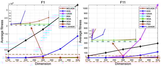
Figure 7.
Scalability analysis for functions.
From Figure 7, it can be seen that for , almost all algorithms can converge to the global optimum in all dimensions, except for the GOA, the PSO, and the L-SHADE. For , the average fitness of MCLAOA, RSA, and WOA are very close as the dimension increases. At dimension 500, the average fitness of MCLAOA is slightly lower than the RSA and the WOA, which is determined by their mathematical models. However, compared to the AOA and the CAOA, the MCLAOA performs the best in all dimensions, which strongly proves that the proposed MCLAOA has been greatly improved. These results demonstrate that the proposed MCLAOA is reliable, especially compared to the AOA and the CAOA, and exhibits excellent performance even when facing high-dimensional optimization problems.
4.4. Results Comparisons Using CEC2020 Benchmark Problems
To further verify the strong competitiveness and optimization applicability of the proposed MCLAOA, we selected a more complex functional benchmark (CEC2020 benchmark problems [48]) and advanced comparison algorithm (the slime mould algorithm, SMA [49] and the hybridizing TLBO with GOA, TLGOA [50]). Due to space limitations, the detailed description and experimental results of CEC2020 are represented in the Appendix A. These CEC2020 benchmark problems can be divided into four types: unimodal functions (), basic functions (–), hybrid functions (–), and composition functions (–). For details on the CEC2020 benchmark problems with a dimension of 10, please refer to Table A1. The parameter settings of SMA and TLGOA are consistent with the original literature [49,50]. Among all the algorithms, the maximum function evaluation with a population size of and for CEC2020 benchmark problems, and they were independently run 30 times. Similar to the 23 benchmark functions, we also adopt , , and as evaluation metrics to assess the optimization performance of all algorithms. The experimental results are shown in Table A2, and the best results are marked in bold type.
From Table A2, it can be observed that the MCLAOA shows the best performance in terms of values on , , , and . The TLGOA performs the best on , , and . The SMA exhibits the best performance on , , and . Furthermore, compared to the standard AOA, the MCLAOA demonstrates significantly better values, indicating its effectiveness in improving optimization performance. It is worth noting that the Friedman rank test for the MCLAOA in Table A2 is 2.3000, ranking first. The p-values corresponding to the Wilcoxon rank-sum test in Table A3 are almost all significantly smaller than 0.05. These results demonstrate that the experimental results obtained from Table A2 are statistically significant. Therefore, the proposed MCLAOA also demonstrates promising performance on more complex benchmark problems.
In summary, we comprehensively analyzed the optimization performance of MCLAOA from several aspects, including accuracy, convergence curve, box plots, statistical analysis, and scalability analysis. These results also lay the foundation for the application of the algorithm to solve more complex optimization problems.
4.5. Engineering Design Problem
To date, we have analyzed the performance of the proposed MCLAOA on unconstrained function benchmarks. Next, we will discuss optimization problems under complex constraint conditions in real-world scenarios. In this paper, two engineering examples, three-bar truss design and a pressure vessel design, are employed to analyze the proposed MCLAOA.
4.5.1. Three-Bar Truss Design Problem
The objective of the three-bar truss design problem is to minimize the weights of the bar structures under certain constraints [16]. The three-bar truss design mainly involves two optimization parameters: the cross-sections with and . There are three constraint conditions, and the mathematical model is shown in the following equations. Here, we compare the proposed MCLAOA with some existing optimization algorithms, and the experimental results are shown in Table 6. The experimental results demonstrate that the proposed MCLAOA exhibits strong competitiveness.
Table 6.
Comparative results for the three-bar truss design problem.
Take ,
Min. ,
Subject to
where
4.5.2. Pressure Vessel Design Problem
The objective of the pressure vessel design problem is to determine the total cost of a cylindrical pressure vessel and minimize the result [16]. The pressure vessel design involves four design variables: the inner radius (R), the thickness of the head (), thickness of the shell (), and the length of the cylindrical part without examining the head (L). There are four constraints, and the mathematical model can be represented by the following equations. Here, we will compare the proposed MCLAOA with some existing optimization algorithms in terms of pressure vessel design, and the experimental results are shown in Table 7. It can be clearly seen that the proposed MCLAOA has significant advantages in solving the pressure vessel design problem.
Table 7.
Comparative results for the pressure vessel design problem.
Take ,
Min. ,
Subject to
5. Application of MCLAOA-BPNN for Cluster Fault Prediction
Due to the rapid development of computer technology, computer systems are widely used in various industries of the national economy [54,55]. Most current software systems can be viewed as cluster systems, which are parallel or distributed systems composed of a large number of independent computers [56]. As the number of nodes in cluster systems continues to increase, the frequency of node failures also increases, which will seriously affect normal usage. In recent years, although existing research work [57,58] in cluster system fault prediction has achieved good results, further improvement is needed in terms of prediction accuracy and efficiency. Therefore, this paper proposed MCLAOA to optimize BPNN parameters and design an MCLAOA-BPNN control cluster fault prediction method.
5.1. Control Cluster System
To meet the demand of uninterrupted and reliable running of multiple computing jobs, a high-availability control cluster system is constructed. The network architecture of the system is shown in Figure 8. The high-availability cluster for multiple computing jobs consists of one central monitoring station and m computing units. Among them, the central monitoring station is responsible for simulating two virtual computers (A and B are backups of each other), completing the monitoring of the high-availability cluster. Each computing unit is responsible for simulating n virtual computers, completing the simulation of computing jobs, dynamic task allocation, migration, and other high availability cluster equipment functions. However, to ensure the sustainable operation of the cluster system, cluster fault prediction is crucial. Therefore, this paper designed a cluster fault prediction method based on BPNN, and used the proposed MCLAOA to optimize the parameters in the BPNN, thus improving the accuracy of cluster fault prediction.
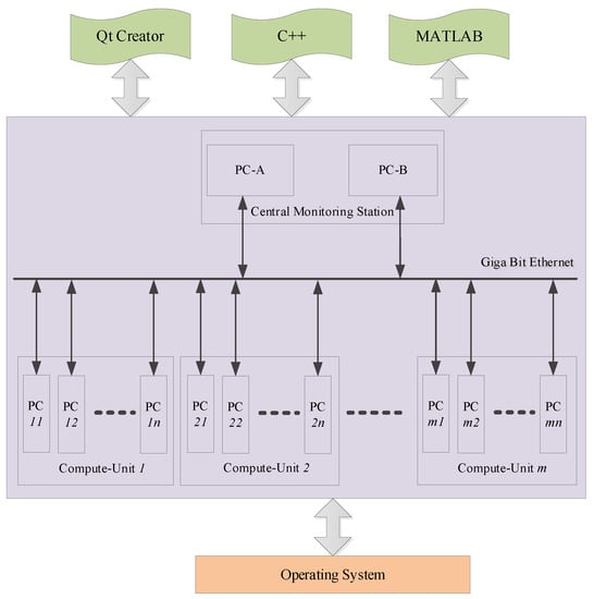
Figure 8.
The network architecture of high-availability control cluster system.
For implementation details, the functions that control the cluster system were implemented using C++. Qt Creator was utilized to showcase these functions via a graphical interface, which also allowed for fault injection to observe the resource information of each PC. The proposed MCLAOA-BPNN was executed on MATLAB, providing fault prediction for the entire cluster system.
5.2. Cluster Fault Prediction Based on MCLAOA-BPNN
5.2.1. BP Neural Network
The computation process of the BPNN consists of a forward computation process and a backward computation process, which includes the input layer, the hidden layer, and the output layer. The BPNN inputs the data from the input layer, processes the data in the hidden layer, and then calculates the difference between the processed data and the true data. If the obtained result does not meet the set error value, it enters the backpropagation process. During backpropagation, the weights and thresholds in each layer of neurons constantly change until the set error value or the predetermined number of training times is reached. The main process of BPNN is as follows:
- Step 1:
- Parameter initialization: the number of nodes in the input layer, the hidden layer, and the output layer, as well as the initial weights and thresholds of each neuron.
- Step 2:
- Forward propagation.
- Step 3:
- Calculation of the error value between the output data and the expected data.
- Step 4:
- Update of the weights and thresholds.
- Step 5:
- Check whether the error value meets the set value. If not, return to Step 4 and update the weights and thresholds until the set error value is reached or the maximum training times are reached.
5.2.2. MCLAOA Optimizes BPNN
During the training process of BPNN, the initial weights and thresholds are randomly generated, which will affect the prediction performance of the model. Therefore, this paper adopts the proposed MCLAOA to optimize the weights and thresholds in BPNN, called MCLAOA-BPNN. The flowchart of the proposed MCLAOA-BPNN cluster fault prediction method is shown in Figure 9, where the red dashed box is the proposed MCLAOA, and the blue dashed box is the MCLAOA-BPNN fault prediction model proposed in this chapter. The specific implementation process is as follows:
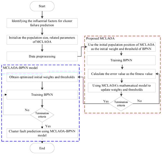
Figure 9.
The flowchart of the MCLAOA-BPNN cluster fault prediction.
- Step 1:
- Analyze the cluster system, determine the fault prediction indicators that affect the cluster system based on the network structure of the cluster system, and construct feature vectors.
- Step 2:
- Initialize the weights and thresholds of BPNN, the parameters of MCLAOA, and read the initial index data of the cluster system as the initial sample data.
- Step 3:
- Pre-process the sample data.
- Step 4:
- Use the MCLAOA to optimize the weights and thresholds of the BPNN and construct the MCLAOA-BPNN fault prediction model.
- Step 5:
- Check whether the termination condition is met. If the termination condition is met, the optimal weights and thresholds are output. Otherwise, skip to Step 4.
- Step 6:
- The optimized weights and thresholds are used as the weights and thresholds of the MCLAOA-BPNN model.
5.3. Experimental Results and Analysis
The high-availability cluster system constructed in this paper has a total of 42 nodes, including 2 central nodes and 40 computing nodes, i.e., . The operating system is Ubuntu 16.04. For the proposed MCLAOA-BPNN fault prediction model, all experiments were performed on MATLAB 2017b, and they were run on a PC with Intel Core i7-10700 2.90 GHz and 16 GB RAM.
We used six main factors that affect cluster performance as sample data, including CPU consumption, memory usage, operating system processes load, net traffic, I/O operations, and number of processes. To simulate faulty behavior, we injected node failures, program errors, network faults, and performance anomalies to obtain fault data. In the data collection process, we collected sample data from 50 moments, normalized the sample data, and used 40 moments as training data and 10 moments as testing data. All data were collected from our own and benchmark (https://ieee-dataport.org/open-access/big-data-machine-learning-benchmark-spark, accessed on 6 June 2019) [59].
5.3.1. Evaluation Criteria
To better evaluate the results of the data, we employed mean absolute error (), root mean square error (), and mean absolute percentage error () as evaluation metrics for the model [60]. The can provide a measure of the overall accuracy of the predictions. The gives more weight to larger errors. The provides a relative measure of the prediction accuracy. The and the are mainly used to measure the degree of difference between predicted values and true values, where the smaller the value, the higher the prediction accuracy of the model. The represents the degree of fluctuation in the difference, where the smaller the value, the more stable the prediction results. The formulas for calculating the , the , and the are as follows:
,
,
,
where N denotes the number of observations, represents the predicted value and is the true value.
5.3.2. Compared Algorithms and Parametric Setup
To evaluate the performance of the proposed MCLAOA-BPNN model, we compared it with the basic BPNN model and swarm-optimized BPNN models (such as the PSO [42], the AOA [16], the CAOA [18], and the sine cosine algorithm (SCA) [61]). In all experiments, the parameter settings were as follows: all population sizes were 50, the number of iterations was 500, and other parameters were set to default values. Additionally, based on the influencing factors, the input layer of the cluster fault prediction model in this paper was set to 6 and the output layer was set to 1. However, the number of hidden layers was not specified, but it is crucial for prediction accuracy. Therefore, we trained the MCLAOA-BPNN cluster fault prediction model with a range of hidden layer numbers (5–12), and the average value of 10 test results for is shown in Table 8, with the best results marked in bold type. It can be seen from Table 8 that the model’s hidden layer was set to 7. Therefore, the final architecture is determined to be a three-layer MCLAOA-BPNN with a configuration of 6-7-1. Furthermore, Figure 10 demonstrates that the proposed model has converged after six epochs, where one epoch refers to the number of training iterations, representing one forward propagation and one backward propagation of the BPNN.
Table 8.
Network training MAE for different numbers of hidden layer nodes.
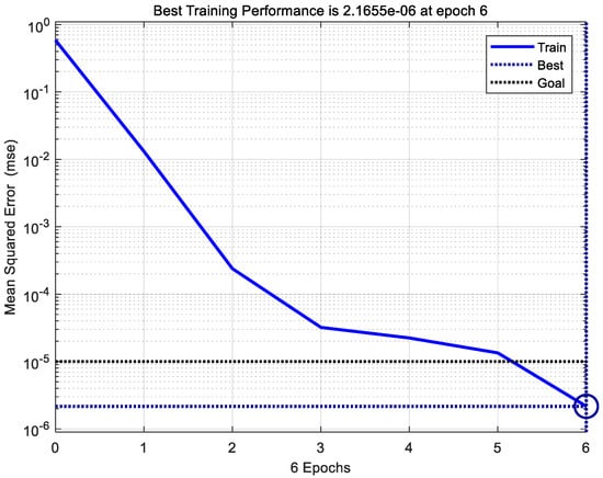
Figure 10.
Number of training samples.
5.3.3. Comparison with other BPNN Models
To verify that the proposed model is highly competitive, we compared MCLAOA-BPNN with other fault prediction models, including the BPNN [62], the PSO-BPNN [42], the AOA-BPNN [16], the CAOA-BPNN [18], and the SCA-BPNN [61]. The errors between the predicted values and true values of different prediction models on different sample data are shown in Figure 11. It can be seen from Figure 11 that the prediction accuracy of BPNN has been improved by swarm-optimized BPNN. The proposed MCLAOA-BPNN shows significant performance, especially compared to the AOA-BPNN and the CAOA-BPNN.
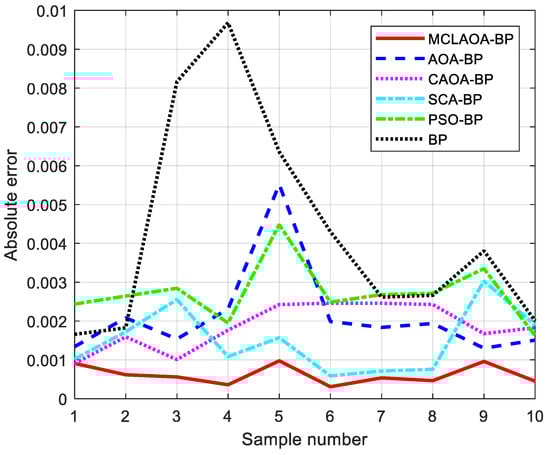
Figure 11.
Comparison of predicted absolute error curves of each model.
In order to clearly observe results, , , and were employed, as shown in Table 9. From Table 9, it can be seen that compared with the AOA-BPNN and the CAOA-BPNN, the proposed MCLAOA-BPNN improves 1.526/1.236, 1.783/1.283, and 0.8762/0.6111 in terms of , , and . Compared with the basic BPNN and the other swarm-optimized BPNN, the proposed MCLAOA-BPNN’s prediction accuracy also ranks first. These results demonstrate that our model can better perform cluster fault prediction.
Table 9.
Predictive results evaluation.
6. Conclusions
In the fault prediction of control cluster systems, the improper setting of initial weights and thresholds in a traditional BPNN can lead to low accuracy. To address this issue, this paper proposes a new swarm intelligence algorithm called MCLAOA and utilizes MCLAOA to optimize the initial weights and thresholds of BPNN, constructing the MCLAOA-BPNN control cluster fault prediction model. To validate the effectiveness of the proposed MCLAOA, 23 benchmark functions, CEC2020 benchmark problems, and two engineering examples were employed. Furthermore, we compared the proposed MCLAOA-BPNN with other swarm-intelligence-based BPNN models to demonstrate its high prediction accuracy.
The following points present the specific experimental results.
- From the last two rows of Table 1, it can be observed that the Friedman rank test of MCLAOA is 2.1034, ranking first. According to the statistical results of the 23 benchmark functions in Table 4, it can be observed that the MCLAOA has improved convergence performance in 16 and 13 functions compared to the basic AOA and LSHADE, respectively.
- The convergence curve and box plots prove that MCLAOA has a faster convergence speed and better robustness.
- Scalability analysis confirms that the MCLAOA has strong and stable performance.
- According to the experimental results of , , and , compared with the basic BPNN/AOA-BPNN, the MCLAOA-BPNN improved by 3.696/1.526, 4.423/1.783, 2.0538/0.8762. Furthermore, the MCLAOA-BPNN outperforms other swarm-intelligence-based BPNN models.
The main limitations of the proposed MCLAOA are as follows: To ensure convergence speed, the MS strategy is only applied in the exploration phase of AOA. Once the algorithm falls into a local optimum during the exploitation phase, it lacks the ability to escape from it. As a result, it exhibits poor performance in handling more complex practical application scenarios such as image processing, engineering design, and other issues. Furthermore, a large number of iterations can increase the computational cost of the fault prediction model. In the future, we plan to introduce mutation operators to enhance the algorithm’s ability to escape local optima. We will also design a convergence monitoring technique to determine whether the desired value has been achieved, whether the expected value is reached, and if so, whether it can terminate iterations and reduce unnecessary losses. Moreover, the proposed MCLAOA can be extended to handle structural optimization, feature selection, etc.
Author Contributions
Conceptualization, T.X. and Z.G.; Methodology, T.X. and Y.Z.; Software, T.X. and Z.G.; Validation, Z.G.; Writing—original draft, T.X.; Writing—review and editing, Z.G. and Y.Z.; Visualization, Y.Z.; Funding acquisition, Y.Z. All authors have read and agreed to the published version of the manuscript.
Funding
This work is supported by the National Natural Science Foundation of China (No.62072235).
Data Availability Statement
The data used to support the findings of this study are available from the corresponding author upon request.
Conflicts of Interest
The authors declare no conflict of interest.
Nomenclature
The following symbols are used in this manuscript:
| t | Current iteration number |
| T | Maximum iteration number |
| Maximum value of the accelerated function | |
| Minimum value of the accelerated function | |
| ∂ | A small integer |
| Upper bound value of the dimension | |
| Lower bound value of the dimension | |
| Control parameter | |
| Sensitive parameter | |
| Step factor | |
| Population size | |
| p | Subpopulation size |
| q | Number of individuals in each subpopulation |
| Inverse function of fitness evaluation | |
| Teacher factor | |
| D | Dimension |
| m | Number of compute-units |
| n | Number of PCs in each compute-unit |
| N | Number of observations |
Appendix A
Table A1.
CEC2020 benchmark problems.
Table A1.
CEC2020 benchmark problems.
| Type | No. | Description | |
|---|---|---|---|
| Unimodal functions | Shifted and Rotated Bent Cigar Function (CEC 2017 ) | 100 | |
| Basic functions | Shifted and Rotated Schwefel’s Function (CEC 2014 ) | 1100 | |
| Shifted and Rotated Lunacek bi-Rastrigin Function (CEC 2017 ) | 700 | ||
| Expanded Rosenbrock’s plus Griewangk’s Function (CEC2017 ) | 1900 | ||
| Hybrid functions | Hybrid Function 1 () (CEC 2014 ) | 1700 | |
| Hybrid Function 2 () (CEC 2017 ) | 1600 | ||
| Hybrid Function 3 () (CEC 2014 ) | 2100 | ||
| Composition functions | Composition Function 1 () (CEC 2017 ) | 2200 | |
| Composition Function 2 () (CEC 2017 ) | 2400 | ||
| Composition Function 3 () (CEC 2017 ) | 2500 |
Table A2.
Numerical results of MCLAOA with other algorithms using CEC2020 benchmark problem.
Table A2.
Numerical results of MCLAOA with other algorithms using CEC2020 benchmark problem.
| Function | Criteria | MCLAOA | AOA | CAOA | RSA | WOA | GOA | SMA | TLGOA |
|---|---|---|---|---|---|---|---|---|---|
| 4.7251E+08 | 6.5860E+09 | 3.9179E+08 | 1.8028E+10 | 2.3351E+05 | 2.2205E+09 | 8.5186E+03 | 5.8672E+06 | ||
| 5.2285E+08 | 2.4988E+09 | 5.0399E+08 | 2.7575E+09 | 5.7869E+05 | 1.7592E+09 | 4.0192E+03 | 1.2834E+07 | ||
| 1.3534E+07 | 1.2835E+09 | 1.2241E+03 | 4.5193E+09 | 1.3832E+04 | 1.4507E+04 | 289.6965 | 1.3823E+06 | ||
| 1.3909E+03 | 1.7983E+03 | 1.8092E+03 | 2.3823E+03 | 2.1676E+03 | 2.1102E+03 | 1.5779E+03 | 1.9750E+03 | ||
| 130.6380 | 183.0234 | 154.0381 | 194.0336 | 287.2063 | 393.2515 | 226.7420 | 283.4210 | ||
| 1.2222E+03 | 1.4506E+03 | 1.4609E+03 | 1.9660E+03 | 1.6097E+03 | 1.2672E+03 | 1.2337E+03 | 1.5287E+03 | ||
| 764.4841 | 804.0515 | 795.0880 | 802.4801 | 779.2079 | 8.8384E+02 | 721.4592 | 726.2413 | ||
| 17.0783 | 6.9201 | 11.4560 | 13.2465 | 26.5078 | 67.9737 | 5.3659 | 8.0244 | ||
| 730.7717 | 794.3927 | 765.6510 | 765.6002 | 741.4918 | 8.1811E+02 | 711.5759 | 711.7954 | ||
| 6.6057E+03 | 9.5217E+03 | 1.6702E+04 | 5.5289E+05 | 2.3003E+04 | 8.5273E+06 | 2.6294E+03 | 1.9512E+03 | ||
| 4.0780E+03 | 7.6283E+03 | 1.2394E+04 | 7.6822E+05 | 4.3024E+04 | 1.6047E+07 | 1.5176E+03 | 50.5600 | ||
| 2.3001E+03 | 2.0331E+03 | 1.9303E+03 | 9.4937E+03 | 2.1231E+03 | 3.1979E+05 | 1.9041E+03 | 1.9075E+03 | ||
| 4.2807E+03 | 4.9853E+04 | 4.2818E+03 | 4.5244E+05 | 1.3354E+05 | 3.2091E+04 | 9.4876E+03 | 3.2977E+03 | ||
| 2.2491E+03 | 2.8177E+04 | 1.0096E+03 | 1.3636E+05 | 2.1080E+05 | 5.5254E+04 | 6.7329E+03 | 5.6970E+03 | ||
| 2.2322E+03 | 1.1207E+04 | 3.1850E+03 | 4.4142E+04 | 5.1664E+03 | 2.7526E+03 | 1.9067E+03 | 1.8024E+03 | ||
| 1.8286E+03 | 1.9828E+03 | 1.9183E+03 | 2.0728E+03 | 1.8357E+03 | 3.0539E+03 | 1.6663E+03 | 1.8319E+03 | ||
| 124.5011 | 138.4976 | 144.2710 | 93.7524 | 117.3325 | 331.0472 | 69.1540 | 132.5534 | ||
| 1.6122E+03 | 1.7364E+03 | 1.6192E+03 | 1.9127E+03 | 1.6397E+03 | 2.4461E+03 | 1.6065E+03 | 1.6400E+03 | ||
| 4.1952E+03 | 5.6449E+03 | 6.2259E+03 | 1.7514E+05 | 3.2918E+04 | 6.9666E+03 | 2.8949E+03 | 2.7665E+03 | ||
| 1.7962E+03 | 2.3694E+03 | 2.6621E+03 | 1.7081E+05 | 3.2594E+04 | 7.5302E+03 | 1.7753E+03 | 410.4163 | ||
| 2.1461E+03 | 2.3547E+03 | 2.3133E+03 | 7.8506E+03 | 4.2554E+03 | 2.4166E+03 | 2.1203E+03 | 2.1776E+03 | ||
| 2.3265E+03 | 2.9057E+03 | 2.5958E+03 | 2.9702E+03 | 2.3315E+03 | 5.7708E+03 | 2.3266E+03 | 2.3581E+03 | ||
| 38.6359 | 315.3173 | 117.4490 | 240.2314 | 15.3485 | 1.9670E+03 | 166.5267 | 237.6234 | ||
| 2.3060E+03 | 2.2885E+03 | 2.3035E+03 | 2.5197E+03 | 2.2393E+03 | 2.4165E+03 | 2.2000E+03 | 2.3045E+03 | ||
| 2.7189E+03 | 2.7927E+03 | 2.7211E+03 | 2.8507E+03 | 2.7519E+03 | 3.0282E+03 | 2.7475E+03 | 2.7426E+03 | ||
| 103.1237 | 88.3431 | 137.8636 | 44.4965 | 77.6254 | 52.7887 | 47.5504 | 102.2214 | ||
| 2.5337E+03 | 2.5774E+03 | 2.5000E+03 | 2.7494E+03 | 2.5045E+03 | 2.9284E+03 | 2.5000E+03 | 2.4563E+03 | ||
| 2.9229E+03 | 3.2008E+03 | 2.9648E+03 | 2.9232E+03 | 2.9583E+03 | 2.9573E+03 | 2.9688E+03 | 2.9410E+03 | ||
| 49.2665 | 145.6641 | 35.1046 | 23.0547 | 31.1292 | 62.4765 | 55.9072 | 29.2071 | ||
| 2.8138E+03 | 2.9688E+03 | 2.8996E+03 | 3.0303E+03 | 2.9011E+03 | 2.8886E+03 | 2.8979E+03 | 2.8986E+03 | ||
| Friedman rank test rank | 2.3000 | 5.6000 | 4.3000 | 7.4000 | 4.7000 | 6.6000 | 2.6000 | 2.5000 | |
| 1 | 6 | 4 | 8 | 5 | 7 | 3 | 2 | ||
Note: The best results of each function were marked in bold type in terms of .
Table A3.
p-values of the Wilcoxon rank-sum test over CEC2020 benchmark problem.
Table A3.
p-values of the Wilcoxon rank-sum test over CEC2020 benchmark problem.
| Function | MCLAOA | AOA | CAOA | RSA | WOA | GOA | SMA | TLGOA |
|---|---|---|---|---|---|---|---|---|
| 3.0199E-11 | 3.0199E-11 | 5.9706E-05 | 3.0199E-11 | 3.0199E-11 | 3.0199E-11 | N/A | 3.0199E-11 | |
| N/A | 6.7220E-10 | 1.7769E-10 | 3.0199E-11 | 4.0772E-11 | 1.1737E-09 | 4.7138E-04 | 2.6099E-10 | |
| 3.3384E-11 | 3.0199E-11 | 3.0199E-11 | 3.0199E-11 | 3.0199E-11 | 3.0199E-11 | N/A | 0.0170 | |
| 3.0199E-11 | 4.9752E-11 | 1.4643E-10 | 3.0199E-11 | 3.0199E-11 | 3.0199E-11 | 0.8534 | N/A | |
| 6.5277E-08 | 7.3891E-11 | 1.0702E-09 | 3.0199E-11 | 1.4643E-10 | 5.5727E-10 | 8.8829E-06 | N/A | |
| 5.0912E-06 | 9.9186E-11 | 3.8249E-09 | 3.0199E-11 | 9.5139E-06 | 3.0199E-11 | N/A | 1.7294E-07 | |
| 0.0163 | 4.1127E-07 | 5.5999E-07 | 3.0199E-11 | 3.0199E-11 | 7.0881E-08 | 0.0032 | N/A | |
| N/A | 5.5727E-10 | 8.8910E-10 | 3.0199E-11 | 0.1453 | 3.3384E-11 | 6.1210E-10 | 0.3871 | |
| N/A | 5.8737E-04 | 0.4463 | 2.2273E-09 | 0.7958 | 3.0199E-11 | 0.0657 | 0.7845 | |
| N/A | 7.3891E-11 | 2.2539E-04 | 3.3384E-11 | 1.1058E-04 | 0.0905 | 2.6806E-04 | 0.0281 |
Note: N/A represents the best algorithm in terms of optimization performance among all the algorithms for the corresponding function.
References
- Saxena, D.; Gupta, I.; Singh, A.K.; Lee, C.N. A fault tolerant elastic resource management framework toward high availability of cloud services. IEEE Trans. Netw. Serv. Manag. 2022, 19, 3048–3061. [Google Scholar] [CrossRef]
- Somasekaram, P.; Calinescu, R.; Buyya, R. High-availability clusters: A taxonomy, survey, and future directions. J. Syst. Softw. 2022, 187, 111208. [Google Scholar] [CrossRef]
- Reisizadeh, A.; Prakash, S.; Pedarsani, R.; Avestimehr, A.S. Coded computation over heterogeneous clusters. IEEE Trans. Inf. Theory 2019, 65, 4227–4242. [Google Scholar] [CrossRef]
- Wael, K.; Jingwei, H. Cluster resource scheduling in cloud computing: Literature review and research challenges. J. Supercomput. 2022, 78, 6898–6943. [Google Scholar]
- Arunarani, A.; Manjula, D.; Sugumaran, V. Task scheduling techniques in cloud computing: A literature survey. Future Gener. Comput. Syst. 2019, 91, 407–415. [Google Scholar] [CrossRef]
- Jena, U.K.; Das, P.K.; Kabat, M.R. Hybridization of meta-heuristic algorithm for load balancing in cloud computing environment—ScienceDirect. J. King Saud Univ. Comput. Inf. Sci. 2022, 34, 2332–2342. [Google Scholar]
- Ghomi, E.J.; Rahmani, A.M.; Qader, N.N. Load-balancing Algorithms in Cloud Computing: A Survey. J. Netw. Comput. Appl. 2017, 88, 50–71. [Google Scholar] [CrossRef]
- Luo, Q.; Hu, S.; Li, C.; Li, G.; Shi, W. Resource Scheduling in Edge Computing: A Survey. IEEE Commun. Surv. Tutorials 2021, 23, 2131–2165. [Google Scholar] [CrossRef]
- Amin, A.A.; Hasan, K.M. A review of Fault Tolerant Control Systems: Advancements and applications. Measurement 2019, 143, 58–68. [Google Scholar] [CrossRef]
- Abbaspour, A.; Mokhtari, S.; Sargolzaei, A.; Yen, K.K. A Survey on Active Fault-Tolerant Control Systems. Electronics 2020, 9, 1513. [Google Scholar] [CrossRef]
- Pinto, J.; Jain, P.; Kumar, T. Hadoop Distributed Computing Clusters for Fault Prediction. In Proceedings of the 2016 International Computer Science and Engineering Conference (ICSEC), Chiang Mai, Thailand, 14–17 December 2016; pp. 1–6. [Google Scholar]
- Mukwevho, M.A.; Celik, T. Toward a Smart Cloud: A Review of Fault-Tolerance Methods in Cloud Systems. IEEE Trans. Serv. Comput. 2021, 14, 589–605. [Google Scholar] [CrossRef]
- Das, D.; Schiewe, M.; Brighton, E.; Fuller, M.; Cerny, T.; Bures, M.; Frajtak, K.; Shin, D.; Tisnovsky, P. Failure Prediction by Utilizing Log Analysis: A Systematic Mapping Study; Association for Computing Machinery: New York, NY, USA, 2020. [Google Scholar]
- Bacanin, N.; Stoean, R.; Zivkovic, M.; Petrovic, A.; Rashid, T.A.; Bezdan, T. Performance of a novel chaotic firefly algorithm with enhanced exploration for tackling global optimization problems: Application for dropout regularization. Mathematics 2021, 9, 2705. [Google Scholar] [CrossRef]
- Malakar, S.; Ghosh, M.; Bhowmik, S.; Sarkar, R.; Nasipuri, M. A GA based hierarchical feature selection approach for handwritten word recognition. Neural Comput. Appl. 2020, 32, 2533–2552. [Google Scholar] [CrossRef]
- Abualigah, L.; Diabat, A.; Mirjalili, S.; Abd Elaziz, M.; Gandomi, A.H. The arithmetic optimization algorithm. Comput. Methods Appl. Mech. Eng. 2021, 376, 113609. [Google Scholar] [CrossRef]
- Yıldız, B.S.; Patel, V.; Pholdee, N.; Sait, S.M.; Bureerat, S.; Yıldız, A.R. Conceptual comparison of the ecogeography-based algorithm, equilibrium algorithm, marine predators algorithm and slime mold algorithm for optimal product design. Mater. Test. 2021, 63, 336–340. [Google Scholar] [CrossRef]
- Li, X.D.; Wang, J.S.; Hao, W.K.; Zhang, M.; Wang, M. Chaotic arithmetic optimization algorithm. Appl. Intell. 2022, 52, 16718–16757. [Google Scholar] [CrossRef]
- Çelik, E. IEGQO-AOA: Information-Exchanged Gaussian Arithmetic Optimization Algorithm with Quasi-opposition learning. Knowl. Based Syst. 2023, 260, 110169. [Google Scholar] [CrossRef]
- Abualigah, L.; Ewees, A.A.; Al-qaness, M.A.; Elaziz, M.A.; Yousri, D.; Ibrahim, R.A.; Altalhi, M. Boosting arithmetic optimization algorithm by sine cosine algorithm and levy flight distribution for solving engineering optimization problems. Neural Comput. Appl. 2022, 34, 8823–8852. [Google Scholar] [CrossRef]
- Mohamed, A.A.; Abdellatif, A.D.; Alburaikan, A.; Khalifa, H.A.E.W.; Elaziz, M.A.; Abualigah, L.; AbdelMouty, A.M. A novel hybrid arithmetic optimization algorithm and salp swarm algorithm for data placement in cloud computing. Soft Comput. 2023, 27, 5769–5780. [Google Scholar] [CrossRef]
- Rajagopal, R.; Karthick, R.; Meenalochini, P.; Kalaichelvi, T. Deep Convolutional Spiking Neural Network optimized with Arithmetic optimization algorithm for lung disease detection using chest X-ray images. Biomed. Signal Process. Control. 2023, 79, 104197. [Google Scholar] [CrossRef]
- Gölcük, İ.; Ozsoydan, F.B.; Durmaz, E.D. An improved arithmetic optimization algorithm for training feedforward neural networks under dynamic environments. Knowl. Based Syst. 2023, 263, 110274. [Google Scholar] [CrossRef]
- Shirazi, M.I.; Khatir, S.; Benaissa, B.; Mirjalili, S.; Wahab, M.A. Damage assessment in laminated composite plates using modal Strain Energy and YUKI-ANN algorithm. Compos. Struct. 2023, 303, 116272. [Google Scholar] [CrossRef]
- Kaveh, A.; Hamedani, K.B. Improved arithmetic optimization algorithm and its application to discrete structural optimization. Structures 2022, 35, 748–764. [Google Scholar] [CrossRef]
- Salimi, H. Stochastic fractal search: A powerful metaheuristic algorithm. Knowl. Based Syst. 2015, 75, 1–18. [Google Scholar] [CrossRef]
- Mirjalili, S. Dragonfly algorithm: A new meta-heuristic optimization technique for solving single-objective, discrete, and multi-objective problems. Neural Comput. Appl. 2016, 27, 1053–1073. [Google Scholar] [CrossRef]
- Guha, D.; Roy, P.; Banerjee, S. Quasi-oppositional symbiotic organism search algorithm applied to load frequency control. Swarm Evol. Comput. 2017, 33, 46–67. [Google Scholar] [CrossRef]
- Truong, K.H.; Nallagownden, P.; Baharudin, Z.; Vo, D.N. A quasi-oppositional-chaotic symbiotic organisms search algorithm for global optimization problems. Appl. Soft Comput. 2019, 77, 567–583. [Google Scholar] [CrossRef]
- Mahajan, S.; Abualigah, L.; Pandit, A.K.; Altalhi, M. Hybrid Aquila optimizer with arithmetic optimization algorithm for global optimization tasks. Soft Comput. 2022, 26, 4863–4881. [Google Scholar] [CrossRef]
- Lalama, Z.; Boulfekhar, S.; Semechedine, F. Localization optimization in wsns using meta-heuristics optimization algorithms: A survey. Wirel. Pers. Commun. 2022, 122, 1197–1220. [Google Scholar] [CrossRef]
- Gad, A.G. Particle swarm optimization algorithm and its applications: A systematic review. Arch. Comput. Methods Eng. 2022, 29, 2531–2561. [Google Scholar] [CrossRef]
- Rahman, M.A.; Sokkalingam, R.; Othman, M.; Biswas, K.; Abdullah, L.; Abdul Kadir, E. Nature-inspired metaheuristic techniques for combinatorial optimization problems: Overview and recent advances. Mathematics 2021, 9, 2633. [Google Scholar] [CrossRef]
- Dhal, K.G.; Sasmal, B.; Das, A.; Ray, S.; Rai, R. A Comprehensive Survey on Arithmetic Optimization Algorithm. Arch. Comput. Methods Eng. 2023, 30, 3379–3404. [Google Scholar] [CrossRef] [PubMed]
- Zhang, H.; Gao, Z.; Zhang, J.; Liu, J.; Nie, Z.; Zhang, J. Hybridizing extended ant lion optimizer with sine cosine algorithm approach for abrupt motion tracking. EURASIP J. Image Video Process. 2020, 2020, 4. [Google Scholar] [CrossRef]
- Gao, Z.; Zhuang, Y.; Chen, C.; Wang, Q. Hybrid modified marine predators algorithm with teaching-learning-based optimization for global optimization and abrupt motion tracking. Multimed. Tools Appl. 2023, 82, 19793–19828. [Google Scholar] [CrossRef]
- Liang, J.J.; Qin, A.K.; Suganthan, P.N.; Baskar, S. Comprehensive learning particle swarm optimizer for global optimization of multimodal functions. IEEE Trans. Evol. Comput. 2006, 10, 281–295. [Google Scholar] [CrossRef]
- Rao, R.V.; Savsani, V.J.; Vakharia, D. Teaching–learning-based optimization: A novel method for constrained mechanical design optimization problems. Comput. Aided Des. 2011, 43, 303–315. [Google Scholar] [CrossRef]
- Abualigah, L.; Abd Elaziz, M.; Sumari, P.; Geem, Z.W.; Gandomi, A.H. Reptile Search Algorithm (RSA): A nature-inspired meta-heuristic optimizer. Expert Syst. Appl. 2022, 191, 116158. [Google Scholar] [CrossRef]
- Mirjalili, S.; Lewis, A. The whale optimization algorithm. Adv. Eng. Softw. 2016, 95, 51–67. [Google Scholar] [CrossRef]
- Saremi, S.; Mirjalili, S.; Lewis, A. Grasshopper optimisation algorithm: Theory and application. Adv. Eng. Softw. 2017, 105, 30–47. [Google Scholar] [CrossRef]
- Kennedy, J.; Eberhart, R. Particle Swarm Optimization. In Proceedings of the ICNN’95-International Conference on Neural Networks, Perth, WA, Australia, 27 November–1 December 1995; pp. 1942–1948. [Google Scholar]
- Tanabe, R.; Fukunaga, A.S. Improving the Search Performance of SHADE Using Linear Population Size Reduction. In Proceedings of the 2014 IEEE Congress on Evolutionary Computation (CEC), Beijing, China, 6–11 July 2014; pp. 1658–1665. [Google Scholar]
- Heidari, A.A.; Mirjalili, S.; Faris, H.; Aljarah, I.; Mafarja, M.; Chen, H. Harris hawks optimization: Algorithm and applications. Future Gener. Comput. Syst. 2019, 97, 849–872. [Google Scholar] [CrossRef]
- Faramarzi, A.; Heidarinejad, M.; Stephens, B.; Mirjalili, S. Equilibrium optimizer: A novel optimization algorithm. Knowl. Based Syst. 2020, 191, 105190. [Google Scholar] [CrossRef]
- Naruei, I.; Keynia, F. Wild horse optimizer: A new meta-heuristic algorithm for solving engineering optimization problems. Eng. Comput. 2022, 38, 3025–3056. [Google Scholar] [CrossRef]
- Derrac, J.; García, S.; Molina, D.; Herrera, F. A practical tutorial on the use of nonparametric statistical tests as a methodology for comparing evolutionary and swarm intelligence algorithms. Expert Syst. Appl. 2011, 1, 3–18. [Google Scholar] [CrossRef]
- Yue, C.T.; Price, K.V.; Suganthan, P.N.; Liang, J.J.; Ali, M.Z.; Qu, B.Y.; Awad, N.H.; Biswas, P.P. Problem Definitions and Evaluation Criteria for the CEC 2020 Special Session and Competition on Single Objective Bound Constrained Numerical Optimization. In Proceedings of the 2020 Genetic and Evolutionary Computation Conference Companion, Cancún, Mexico, 8–12 July 2020. [Google Scholar]
- Li, S.; Chen, H.; Wang, M.; Heidari, A.A.; Mirjalili, S. Slime mould algorithm: A new method for stochastic optimization. Future Gener. Comput. Syst. 2020, 111, 300–323. [Google Scholar] [CrossRef]
- Zhang, H.; Gao, Z.; Ma, X.; Zhang, J.; Zhang, J. Hybridizing teaching-learning-based optimization with adaptive grasshopper optimization algorithm for abrupt motion tracking. IEEE Access 2019, 7, 168575–168592. [Google Scholar] [CrossRef]
- Zheng, R.; Jia, H.; Abualigah, L.; Liu, Q.; Wang, S. An improved arithmetic optimization algorithm with forced switching mechanism for global optimization problems. Math. Biosci. Eng 2022, 19, 473–512. [Google Scholar] [CrossRef]
- Yang, Y.; Gao, Y.; Tan, S.; Zhao, S.; Wu, J.; Gao, S.; Zhang, T.; Tian, Y.C.; Wang, Y.G. An opposition learning and spiral modelling based arithmetic optimization algorithm for global continuous optimization problems. Eng. Appl. Artif. Intell. 2022, 113, 104981. [Google Scholar] [CrossRef]
- Faramarzi, A.; Heidarinejad, M.; Mirjalili, S.; Gandomi, A.H. Marine Predators Algorithm: A nature-inspired metaheuristic. Expert Syst. Appl. 2020, 152, 113377. [Google Scholar] [CrossRef]
- Catal, C. Software fault prediction: A literature review and current trends. Expert Syst. Appl. 2011, 38, 4626–4636. [Google Scholar] [CrossRef]
- Ahmed, Q.; Raza, S.A.; Al-Anazi, D.M. Reliability-based fault analysis models with industrial applications: A systematic literature review. Qual. Reliab. Eng. Int. 2021, 37, 1307–1333. [Google Scholar] [CrossRef]
- Agrawal, A. Concepts for distributed systems design. Proc. IEEE 1986, 74, 236. [Google Scholar] [CrossRef]
- Shafiq, M.; Alghamedy, F.H.; Jamal, N.; Kamal, T.; Daradkeh, Y.I.; Shabaz, M. Scientific programming using optimized machine learning techniques for software fault prediction to improve software quality. IET Software 2023, 1–11. [Google Scholar] [CrossRef]
- Tameswar, K. Towards Optimized K Means Clustering Using Nature-Inspired Algorithms for Software Bug Prediction. Available online: https://ssrn.com/abstract=4358066 (accessed on 14 February 2023).
- Jairson, R.; Germano, V. Big Data Machine Learning Benchmark on Spark. IEEE Dataport 2019. [Google Scholar] [CrossRef]
- Al-Musaylh, M.S.; Deo, R.C.; Li, Y.; Adamowski, J.F. Two-phase particle swarm optimized-support vector regression hybrid model integrated with improved empirical mode decomposition with adaptive noise for multiple-horizon electricity demand forecasting. Appl. Energy 2018, 217, 422–439. [Google Scholar] [CrossRef]
- Mirjalili, S. SCA: A sine cosine algorithm for solving optimization problems. Knowl.-Based Syst. 2016, 96, 120–133. [Google Scholar] [CrossRef]
- Rumelhart, D.E.; Hinton, G.E.; Williams, R.J. Learning representations by back-propagating errors. Nature 1986, 323, 533–536. [Google Scholar] [CrossRef]
Disclaimer/Publisher’s Note: The statements, opinions and data contained in all publications are solely those of the individual author(s) and contributor(s) and not of MDPI and/or the editor(s). MDPI and/or the editor(s) disclaim responsibility for any injury to people or property resulting from any ideas, methods, instructions or products referred to in the content. |
© 2023 by the authors. Licensee MDPI, Basel, Switzerland. This article is an open access article distributed under the terms and conditions of the Creative Commons Attribution (CC BY) license (https://creativecommons.org/licenses/by/4.0/).