Unit Distributions: A General Framework, Some Special Cases, and the Regression Unit-Dagum Models

Abstract

In this work, we propose a general framework for models with support in the unit interval, which is obtained using the technique of random variable transformations. For this class, the general expressions of distribution and density functions are given, together with the principal characteristics, such as quantiles, moments, and hazard and reverse hazard functions. It is possible to verify that different proposals already present in the literature can be seen as particular cases of this general structure by choosing a suitable transformation. Moreover, we focus on the class of unit-Dagum distributions and, by specifying two different kinds of transformations, we propose the type I and type II unit-Dagum distributions. For these two models, we first consider the possibility of expressing the distribution in terms of indicators of interest, and then, through the regression approach, relate the indicators and covariates. Finally, some applications using data on the unit interval are reported.

1. Introduction

In statistical literature, several authors have focused their attention on developing new and more flexible statistical distributions by using suitable transformation techniques (see, for example, [1,2,3]). Most of the obtained distributions deal with continuous random variables with unbounded support. Only in recent years has attention been devoted to filling the existing gap with respect to distributions with bounded support, in order to meet the need to describe empirical phenomena whose realizations cover limited ranges. Indeed, these kinds of data naturally arise in different contexts, such as rates, proportions, percentages, and so on, but just a few models, such as the widely used beta distribution model, the Kumaraswamy model [4], the Topp–Leone model [5], the arcsine model [6], the standard two-sided power model [7], and a few more (see [8,9]) were available in the past to describe them. Many others are very recent proposals. In particular, in the last decade, there have been many works in this field, for the most part, on models belonging to the class of so-called unit distributions. These models describe data with support in unit intervals and are often obtained by applying transformations to random variables. These include the unit-Burr III [10,11], unit-Lindley [12], unit-Gompertz [13], unit-Burr XII [14], unit inverse Gaussian [15], the arcsecant hyperbolic normal model [16], and logit slash [17], to name a few, as well as some new families of distributions [18,19].

The first aim of this work is to describe a general structure based on the random variable transformation technique, which includes most of the distributions for data on unit intervals already present in the literature. Moreover, other members of this class were obtained, considering different transformations. Particular attention is placed on building regression models, starting with unit distributions; this allows us to evaluate the impact of covariates on response variables with bounded support and consider alternative approaches to the most used regression models for unit data.

In a recent paper, [20] proposed a unified procedure to construct distribution functions in the (0,1) interval from the composition of two random variables with the same support, which turned out to be a special case of the $T-X$ family introduced by [21]. Our approach differs from the one just mentioned in that it does not require the knowledge of a second distribution function or a second quantile function. Furthermore, we envisaged a reparameterization and construction of the regression models on the indicators of interest.

The rest of the paper is organized as follows. In Section 2, we define the general class of distributions and derive the expressions for distribution and probability density functions. Quantiles, moments, and general expressions for the hazard and reverse hazard rate are given. A particular case of distributions belonging to the general class is described in Section 3, starting with the Dagum random variable and considering two particular kinds of transformations. The maximum likelihood estimation is discussed in Section 4. Section 5 is devoted to showing the possibility of employing the proposed models according to a regression perspective. Finally, in Section 6, two different examples of applications are shown.

2. General Framework

Many of the recently suggested distributions, proposed for modeling data belonging to the unit interval, can be described by resorting to a single probabilistic structure based on a simple technique of a random variable transformation.

To this end, let Y be a random variable (rv) with a distribution function (pdf) $F_Y(y;\mathit{\theta })$ and probability density function (df) $F_Y(y;\mathit{\theta })$, where $\mathit{\theta }$ is the parameter vector and $y\in S_Y\subset \Re$, $S_Y=[{\underline{S}}_Y,{\overline{S}}_Y]$. Let $C:S_Y⟼J_V$ be the application that identifies the transformation of Yrv in a new variable V, assuming values $V\in J_V=[{\underline{J}}_V,{\overline{J}}_V]$. In general, the distribution of V could also be characterized by a vector of parameters $\mathit{a}$, i.e., $V:=C(Y;\mathbf{a})$.

In the present paper, in order to simplify the discussion, we assume that the boundaries of the support of V are finite, i.e., ${lim}_{y\to {\underline{S}}_Y}C(y;\mathbf{a})={\underline{J}}_V>-\infty$ and ${lim}_{y\to {\overline{S}}_Y}C(y;\mathbf{a})={\overline{J}}_V<\infty$, and we assume that the function $C(y;\mathbf{a})$ is continuous, differentiable, and monotone over $S_Y$. Consequently, $C(y;\mathbf{a})$ is invertible and its inverse $C^{-1}(·)$ is differentiable on $J_V$:

$${\left(C^{-1}(v;\mathbf{a})\right)}^{\prime }=\frac{1}{C^{\prime }\left(C^{-1}(v;\mathbf{a})\right)}.$$

(1)

Knowing the distribution function of Y and considering the transformation $C(·)$, it is easy to obtain the distribution function of V and its characteristics, such as quantiles and moments. Moreover, it is typical in the literature to study the behavior of the hazard function $h_Y(y;\mathit{\theta })$ (hf) and the reverse hazard function (rhf) $r{h}_Y(y;\mathit{\theta })$, with the aim of evaluating the flexibility of a distribution. Therefore, in the following, we obtain some general expressions of characteristics and properties for distributions belonging to this class. In doing this, we distinguish two cases, depending on whether $C(·)$ is an increasing or a decreasing monotonic function.

(1)

$C(·)$ is an increasing monotonic function:

the $df$ of V is given by:

$$F_V(v;\mathit{\theta },\mathbf{a})=P(V\le v)=P\left(Y\le C^{-1}(v;\mathbf{a})\right)=F_Y\left(C^{-1}(v;\mathbf{a});\mathit{\theta }\right)$$

(2)

and, by (1), we can obtain the $pdf$ of V as

$$f_V(v;\mathit{\theta },\mathbf{a})=\frac{\partial F_Y\left(C^{-1}(v;\mathbf{a});\mathit{\theta }\right)}{\partial C^{-1}(v;\mathbf{a})}\times \frac{\partial C^{-1}(v;\mathbf{a})}{\partial v}=\frac{f_Y\left(C^{-1}(v;\mathbf{a});\mathit{\theta }\right)}{C^{\prime }\left(C^{-1}(v;\mathbf{a})\right)}.$$

(3)

Moreover, let $y\left(p\right)=F_Y^{-1}(y;\mathit{\theta })$ be the p-th quantile of Y, with $p\in (0,1)$. It is easy to verify that, from (2), the q-th quantile of V is as follows:

$$v(q;\mathit{\theta },\mathbf{a})=C\left(y(q;\mathit{\theta });\mathbf{a}\right),$$

(4)

with $q\in (0,1)$.

The general expressions for $hr$ and $rhr$ functions are, respectively, given by:

$$h_V(v;\mathit{\theta },\mathbf{a})=\frac{f_V(v;\mathit{\theta },\mathbf{a})}{1-F_V(v;\mathit{\theta },\mathbf{a})}=\frac{h_Y(C^{-1}(v;\mathbf{a});\mathit{\theta })}{C^{\prime }\left(C^{-1}(v;\mathbf{a})\right)}$$

(5)

$$r{h}_V(v;\mathit{\theta },\mathbf{a})=\frac{f_V(v;\mathit{\theta },\mathbf{a})}{F_V(v;\mathit{\theta },\mathbf{a})}=\frac{r{h}_Y(C^{-1}(v;\mathbf{a});\mathit{\theta })}{C^{\prime }\left(C^{-1}(v;\mathbf{a})\right)}.$$

(6)

(2)

$C(.)$ is a decreasing monotonic function.

In this case, with little algebra, we can determine the quantities previously considered. In particular, the df and pdf of V, respectively, are as follows:

$$F_V(v;\mathit{\theta },\mathbf{a})=1-F_Y\left(C^{-1}(v;\mathbf{a});\mathit{\theta }\right),$$

$$f_V(v;\mathit{\theta },\mathbf{a})=-\frac{f_Y\left(C^{-1}(v;\mathbf{a});\mathit{\theta }\right)}{C^{\prime }\left(C^{-1}(v;\mathbf{a})\right)}$$

and the quantile of order q is as follows:

$$v(q;\mathit{\theta },\mathbf{a})=C\left(y(1-q;\mathit{\theta });\mathbf{a}\right).$$

The hf and rhf are calculated accordingly.

We can use different methods, known in the literature, to determine the moment of order r.

We should note that most of the proposals in the literature can be thought of as particular cases of the comprehensive framework described earlier. For example, the most used transformations in the cases of positive rvs are as follows: $V=\frac{Y}{1+Y}$ and $V=e^{-Y}$. On the other hand, the most common transformation, when Y assumes a real value, is $V=\frac{1}{1+e^{-Y}}$, as in the case of the logit slash model. Moreover, $V=\frac{2}{e^{-Y}+e^Y}$ was used in the context of non-monotonic rv transformations to obtain the arcsecant hyperbolic normal model, which, strictly speaking, does not belong to the general framework proposed here, but it can be used in every case with small mathematical expedients. We should note that, in general, any distribution function $G(·)$ can be used to transform Yrv in a new variable $V=G\left(Y\right)$. Table 1 summarizes a classification of some unit distributions proposed in the literature, according to the used transformation.

Table 1. Unit distributions proposed in the literature according to the used transformation.

Distribution, Reference	$\mathit{C}(\mathit{Y};\mathit{a})$	${\mathit{f}}_{\mathit{V}}(\mathit{v};\mathit{\theta };\mathit{a})$	Parameter Space
Unit-Burr III, [10]	$Y/(1+Y)$	${\theta }_1{\theta }_2{\left[1+{\left(\frac{1}{v}-1\right)}^{{\theta }_2}\right]}^{-{\theta }_1-1}{\left(\frac{1}{v}-1\right)}^{{\theta }_2-1}\frac{1}{v^2}$	${\theta }_1,{\theta }_2>0$
Unit-Half-Normal, [22]	$Y/(1+Y)$	$\frac{2}{\theta {(1-v)}^2}\varphi \left(\frac{v}{\theta (1-v)}\right)$	$\theta >0$
Unit-modified Burr III, [23]	$Y/(1+Y)$	${\theta }_1{\theta }_2{v}^{-2}{\left(\frac{1-v}{v}\right)}^{{\theta }_2-1}{\left[1+{\theta }_3{\left(\frac{1-v}{v}\right)}^{{\theta }_2}\right]}^{-\frac{{\theta }_1}{{\theta }_3}-1}$	${\theta }_1,{\theta }_2,{\theta }_3>0$
Unit-Lindley, [12]	$Y/(1+Y)$	$\frac{{\theta }^2}{1+\theta }{(1-v)}^{-3}exp\left(-\frac{\theta v}{1-v}\right)$	$\theta >0$
Unit-Gompertz, [13]	$exp\{-Y\}$	${\theta }_1{\theta }_2{v}^{-({\theta }_2+1)}exp\left[-{\theta }_1(v^{-{\theta }_2}-1)\right]$	${\theta }_1,{\theta }_2>0$
Unit-Birnbaum-Saunders, [24,25]	$exp\{-Y\}$	$\frac{1}{2v{\theta }_1{\theta }_2\sqrt{2\pi }}\left[{\left(-\frac{{\theta }_2}{logv}\right)}^{1/2}+{(-\frac{{\theta }_2}{logv})}^{3/2}\right]exp\left[\frac{1}{2{\theta }_1^2}(\frac{logv}{{\theta }_2}+\frac{{\theta }_2}{logv}+2)\right]$	${\theta }_1,{\theta }_2>0$
Bounded Odd inv. Pareto exp., [26]	$exp\{-Y\}$	$\frac{{\theta }_1{\theta }_2{\theta }_3{v}^{{\theta }_3-1}{(1-v^{{\theta }_3})}^{{\theta }_1-1}}{{(1-(1-{\theta }_2)v^{{\theta }_3})}^{{\theta }_1+1}}$	${\theta }_1,{\theta }_2,{\theta }_3>0$
Unit-Burr XII, [14]	$exp\{-Y\}$	${\theta }_1{\theta }_2{v}^{-1}{(-logv)}^{{\theta }_2-1}{\left(1+{(-logv)}^{{\theta }_2}\right)}^{-{\theta }_1-1}$	${\theta }_1,{\theta }_2>0$
Log-Bilal, [27]	$exp\{-Y\}$	$\frac{6}{\theta }{v}^{2/\theta -1}\left(1-v^{1/\theta }\right)$	$\theta >0$
Unit-inverse Gaussian, [15]	$exp\{-Y\}$	$\sqrt{\frac{{\theta }_1}{2\pi }}\frac{1}{v{(-logv)}^{3/2}}exp\left[-\frac{{\theta }_1}{2{\left({\theta }_2\right)}^{2}logv}{(logv+{\theta }_2)}^2\right]$	${\theta }_1,{\theta }_2>0$
Unit-Burr III, [11]	$exp\{-Y\}$	${\theta }_1{\theta }_2\frac{{\left(log(1/v)\right)}^{-{\theta }_2-1}}{v{(1+{\left(log(1/v)\right)}^{-{\theta }_2})}^{{\theta }_1+1}}$	${\theta }_1,{\theta }_2>0$
Logit slash, [17]	$1/[1+exp\{-Y\left\}\right]$	$\frac{{\theta }_1}{v(1-v){\theta }_3}{\int }_0^1{t}^{{\theta }_1}\varphi \left(t\left[\frac{log\left(\frac{v}{1-v}\right)-{\theta }_2}{\theta 3}\right]\right)dt$	${\theta }_1,{\theta }_3>0;-\infty <{\theta }_2<\infty$

In many application contexts, researchers often focus on specific aspects when characterizing a distribution, such as quantiles, location measures (mode, median, mean), variability indicators, etc. For this reason, when possible, it is useful to express the distribution as a function of such characteristics. The utility derives from the fact that, with appropriate methodological tools, it is possible to construct regressive models on the characteristics of interest with the aim of inspecting the possible determinants of the phenomenon under investigation (see [28,29]). Each characteristic and/or indicator is, in general, a function of the vector of the distribution parameters, let us say $I=I\left(\mathit{\theta }\right)$, with reference to the unit’s distribution function (2). If $\mathit{\theta }$ is a vector of dimension p and the system

$$\begin{array}{c}\hfill I_j=I_j({\theta }_1,{\theta }_2,\dots ,{\theta }_p)forj=1,\dots ,p\end{array}$$

has a unique finite solution, say,

$$\begin{array}{c}\hfill {\theta }_j={\theta }_j(I_1,I_2,\dots ,I_p)forj=1,\dots ,p\end{array}$$

then the unit-distribution function

$$\begin{array}{c}\hfill F_V\left(v;I_1,I_2,\dots ,I_p\right)=F_V(v;{\theta }_1(I_1,I_2,\dots ,I_p),{\theta }_2(I_1,I_2,\dots ,I_p),\dots ,{\theta }_p(I_1,I_2,\dots ,I_p))\end{array}$$

represents a reparameterization in terms of indicators and/or characteristics of interest of the distribution in (2).

3. Two Kinds of Unit-Dagum Distributions

In this section, two different transformations of the widely used Dagum rv [30,31] will be described. Given the ability of the Dagum model in fitting real data, the resulting new models may potentially be more flexible than unit distributions that have already appeared in the literature.

The df and pdf of Dagum rv Y are given, respectively, by:

$$\begin{array}{c}\hfill F_{Da}(y;\beta ,\lambda ,\delta )={\left(1+\lambda y^{-\delta }\right)}^{-\beta },\end{array}$$

(7)

and

$$\begin{array}{c}\hfill f_{Da}(y;\beta ,\lambda ,\delta )=\beta \lambda \delta y^{-\delta -1}{\left(1+\lambda y^{-\delta }\right)}^{-\beta -1},\end{array}$$

(8)

with $y>0$ and $\beta ,\lambda ,\delta >0$. In particular, the vector of parameters of Dagum distribution (hereafter, $Da(\beta ,\delta ,\lambda )$) is $\mathit{\theta }=(\beta ,\lambda ,\delta )$, where $\lambda$ represents a scale parameter and $\beta$ and $\delta$ are shape parameters.

The Dagum model is positively skewed and it can be unimodal or zero-modal, depending on $\beta \delta >1$ or $\beta \delta \le 1$. In particular, the mode is given by

$$y_m={\lambda }^{\frac{1}{\delta }}{\left(\frac{\beta \delta -1}{\delta +1}\right)}^{\frac{1}{\delta }}.$$

(9)

It is easy to verify that the q-th quantile is

$$y\left(q\right)=F_{Da}^{-1}(q;\beta ,\lambda ,\delta )={\lambda }^{\frac{1}{\delta }}{(q^{-\frac{1}{\beta }}-1)}^{-\frac{1}{\delta }},$$

(10)

therefore, the expression of the median is explicit:

$$me={\lambda }^{\frac{1}{\delta }}{(2^{\frac{1}{\beta }}-1)}^{-\frac{1}{\delta }}.$$

(11)

It is also possible to obtain the expression of the r-th moment, as follows

$${\mu }_{Da}^r=E(Y^r;\beta ,\lambda ,\delta )=\beta {\lambda }^{\frac{r}{\delta }}B\left(\beta +\frac{r}{\delta },1-\frac{r}{\delta }\right),$$

(12)

which exists for $\delta >r$. Here, $B(·,·)$ indicates the complete beta function.

3.1. The First Kind of Unit-Dagum Distribution

In this section, we consider the hyperbolic secant transformation:

$$V:=C\left(Y\right)=\frac{2e^Y}{1+e^{2Y}}.$$

In particular, it is simple to verify that, for $Y>0$, it is a monotonic decreasing function with ${lim}_{y\to 0^{+}}C\left(y\right)=1$, ${lim}_{y\to +\infty }C\left(y\right)=0$ and $C^{\prime }\left(y\right)=\frac{2e^y\left(1-e^{2y}\right)}{{\left(1+e^{2y}\right)}^2}<0$. Furthermore, it is known that the inverse hyperbolic secant is given by $y=C^{-1}\left(v\right)=log\frac{1+\sqrt{1-v^2}}{v}$.

Taking into account the characteristics of the proposed transformation, the distribution function of the new rv V is given by

$$\begin{array}{ccc}\hfill F_{I-UDa}(v;\beta ,\lambda ,\delta )& =& 1-F_{Da}(log\frac{1+\sqrt{1-v^2}}{v};\beta ,\lambda ,\delta )\hfill \\ & =& 1-{\left\{1+\lambda {\left[log\frac{1+\sqrt{1-v^2}}{v}\right]}^{-\delta }\right\}}^{-\beta }\hfill \end{array}$$

(13)

with $v\in (0,1)$ and $\beta ,\lambda ,\delta >0$ (hereafter, $I-UDa(\beta ,\delta ,\lambda )$). From (1), after simple algebra, we obtain the first derivative of the inverse of $C(y;\mathit{a})$:

$${\left(C^{-1}(v;\mathbf{a})\right)}^{\prime }=\frac{-1}{v\sqrt{1-v^2}}$$

and, consequently, the pdf of $I-UDa(\beta ,\delta ,\lambda )$ rv:

$$\begin{array}{c}\hfill f_{I-UDa}(v;\beta ,\lambda ,\delta )=\frac{\beta \lambda \delta }{v\sqrt{1-v^2}}{\left[log\left(v^{*}\right)\right]}^{-\delta -1}{\left\{1+\lambda {\left[log\left(v^{*}\right)\right]}^{-\delta }\right\}}^{-\beta -1}\end{array}$$

(14)

where $v^{*}=\frac{1+\sqrt{1-v^2}}{v}$.

Figure 1 shows various behaviors of the pdf for the type I unit-Dagum model, according to different values of parameters.

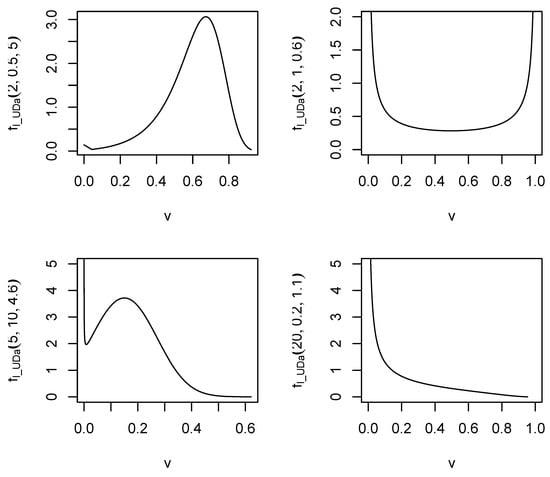
Figure 1. Pdf of the type I unit-Dagum model for different values of parameters.

The q-th quantile of the $I-UDa(\beta ,\delta ,\lambda )$ distribution, by (10), is

$$\begin{array}{c}\hfill v(q;\beta ,\lambda ,\delta )=\frac{2e^{{\lambda }^{\frac{1}{\delta }}{\left({(1-q)}^{-\frac{1}{\beta }}-1\right)}^{-\frac{1}{\delta }}}}{1+e^{2{\lambda }^{\frac{1}{\delta }}{\left({(1-q)}^{-\frac{1}{\beta }}-1\right)}^{-\frac{1}{\delta }}}}.\end{array}$$

(15)

In the following proposition, we show that the r-th moment of the type I unit-Dagum distribution can be expressed in terms of moments of the Dagum distribution.

Proposition 1.

The r-th moment of $V\sim I-UDa(\beta ,\delta ,\lambda )$ has the following expression:

$$\begin{array}{c}\hfill E\left[V^r\right]=\beta 2^r{\displaystyle \sum _{j=0}^{+\infty }}\left(\genfrac{}{}{0pt}{}{-r}{j}\right){\displaystyle \sum _{s=0}^{+\infty }}\frac{{(-1)}^s}{s!}{\left(2j+r\right)}^s{\lambda }^{s}B\left(\beta +\frac{s}{\delta },1-\frac{s}{\delta }\right).\end{array}$$

(16)

Proof. 

See Appendix A.1.    □

The hf and rhz are given, respectively, by 

$$\begin{array}{c}\hfill h{f}_{I-UDa}(v;\beta ,\lambda ,\delta )=\frac{\beta \lambda \delta }{v\sqrt{1-v^2}\left[log\left(v^{*}\right)\right]\left\{\lambda +{\left[log\left(v^{*}\right)\right]}^{\delta }\right\}}\end{array}$$

(17)

and

$$\begin{array}{c}\hfill rh{f}_{I-UDa}(v;\beta ,\lambda ,\delta )=\frac{\beta \lambda \delta {\left[log\left(v^{*}\right)\right]}^{-\delta -1}{\left\{1+\lambda {\left[log\left(v^{*}\right)\right]}^{-\delta }\right\}}^{-\beta -1}}{v\sqrt{1-v^2}\left[1-{\left\{1+\lambda {\left[log\frac{1+\sqrt{1-v^2}}{v}\right]}^{-\delta }\right\}}^{-\beta }\right]}\end{array}$$

(18)

The hazard rate function of the type I unit-Dagum model for some values of parameters is shown in Figure 2.

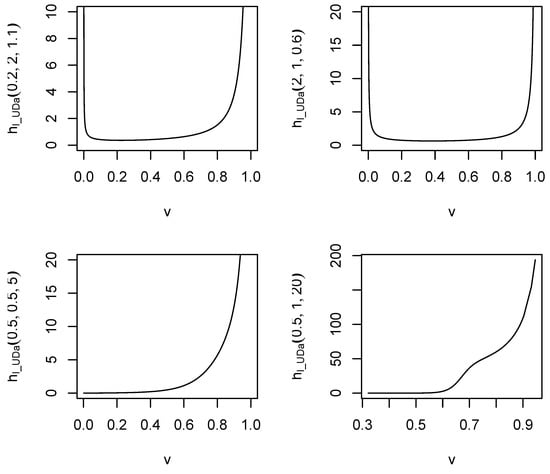
Figure 2. Hazard rate of the type I unit-Dagum model for different values of parameters.

We propose a possible reparametrization of the type I unit-Dagum distribution in terms of the median and the $q-th$ quantile. It is possible to verify that the system

$$\left\{\begin{array}{c}{\beta }_1=\frac{1}{\beta }\hfill \\ me=\frac{2e^{{\lambda }^{\frac{1}{\delta }}{\left[{0.5}^{-\frac{1}{\beta }}-1\right]}^{-\frac{1}{\delta }}}}{1+e^{2{\lambda }^{\frac{1}{\delta }}{\left[{0.5}^{-\frac{1}{\beta }}-1\right]}^{-\frac{1}{\delta }}}}\hfill \\ v\left(q\right)=\frac{2e^{{\lambda }^{\frac{1}{\delta }}{\left[{(1-q)}^{-\frac{1}{\beta }}-1\right]}^{-\frac{1}{\delta }}}}{1+e^{2{\lambda }^{\frac{1}{\delta }}{\left[{(1-q)}^{-\frac{1}{\beta }}-1\right]}^{-\frac{1}{\delta }}}}\hfill \end{array}\right.$$

(19)

presents the following unique solution:

$$\left\{\begin{array}{c}\beta =\frac{1}{{\beta }_1}\hfill \\ \lambda =\left[{0.5}^{-{\beta }_1}-1\right]{\left[log\left(\frac{1+\sqrt{1-m{e}^2}}{me}\right)\right]}^{{\delta }^{*}}={\lambda }^{*}\hfill \\ \delta =\frac{log\left[{0.5}^{-{\beta }_1}-1\right]-log\left[{(1-q)}^{-{\beta }_1}-1\right]}{log\left[log\left(\frac{1+\sqrt{1-v{\left(q\right)}^2}}{v\left(q\right)}\right)\right]-log\left[log\left(\frac{1+\sqrt{1-m{e}^2}}{me}\right)\right]}={\delta }^{*}\hfill \end{array}\right.$$

(20)

The corresponding distribution function is

$$\begin{array}{c}\hfill F_{R-I-UDa}(v;{\beta }_1,me,v\left(q\right))=1-{\left\{1+{\lambda }^{*}{\left[log\frac{1+\sqrt{1-v^2}}{v}\right]}^{-{\delta }^{*}}\right\}}^{-\frac{1}{{\beta }_1}}\end{array}$$

(21)

with ${\beta }_1>0$, $me\in (0,1)$ and $v\left(q\right)\in (0,1)$ for $q\in (0,1)$.

3.2. A Second Kind of Unit-Dagum Distribution

In this section, we consider the monotonic decreasing transformation $V:=C\left(Y\right)=e^{-Y}$, with ${lim}_{y\to 0^{+}}C\left(y\right)=1$, ${lim}_{y\to +\infty }C\left(y\right)=0$ and $C^{\prime }\left(y\right)=-e^{-y}<0$, $\forall y$. The inverse is given by $y=C^{-1}\left(v\right)=-log\left(v\right)$.

The distribution function of V is given by

$$\begin{array}{ccc}\hfill F_{II-UDa}(v;\beta ,\lambda ,\delta )& =& 1-F_{Da}(-logv;\beta ,\lambda ,\delta )\hfill \\ & =& 1-{\left\{1+\lambda {\left[-log\left(v\right)\right]}^{-\delta }\right\}}^{-\beta }\hfill \end{array}$$

(22)

with $v\in (0,1)$ and $\beta ,\lambda >0,\delta >0$ (hereafter, $II-UDa(\beta ,\delta ,\lambda )$). From (1), after simple algebra, we obtain the first derivative of the inverse of $C(y;\mathbf{a})$:

$${\left(C^{-1}(v;\mathbf{a})\right)}^{\prime }=-\frac{1}{v}$$

and, consequently, the pdf of $II-UDa(\beta ,\lambda ,\delta )$ rv:

$$\begin{array}{c}\hfill f_{II-UDa}(v;\beta ,\lambda ,\delta )=\frac{\beta \lambda \delta }{v}{\left[-log\left(v\right)\right]}^{-\delta -1}{\left\{1+\lambda {\left[-log\left(v\right)\right]}^{-\delta }\right\}}^{-\beta -1}.\end{array}$$

(23)

It is worth noting that the distribution in (23) can be viewed as an extension of the unit-Burr III obtained by [11], using the same transformation. Indeed, the Dagum model has one more parameter than Burr III, that is a scale parameter, thus, by putting $\lambda =1$, the unit-Burr III is obtained. Although the unit-Burr III is already studied in the literature, for the purposes of this work, as will be seen later, the  $\lambda$ parameter is essential for carrying out the reparameterization and building the regression model; therefore, here, we consider the type II unit-Dagum distribution, also considering the scale parameter.

Figure 3 shows various behaviors of the pdf for the type II unit-Dagum model according to different parameter values.

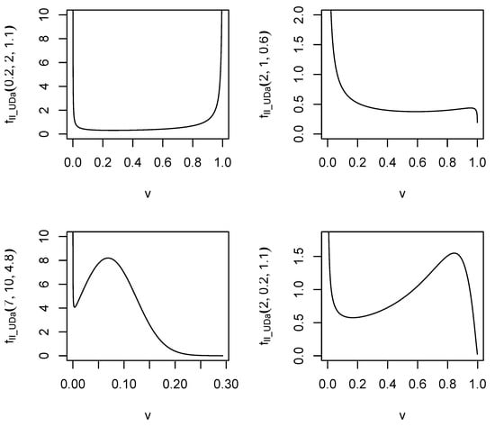
Figure 3. Pdf of II-UDa for different values of parameters.

The q-th quantile of the $II-UDa(\beta ,\delta ,\lambda )$ distribution, by (10), is

$$\begin{array}{c}\hfill v(q;\beta ,\lambda ,\delta )=e^{-{\lambda }^{1/\delta {\left[{(1-q)}^{-1\beta }-1\right]}^{-1/\delta }}}.\end{array}$$

(24)

It can be readily verified that the r-th moment of the type II unit-Dagum distribution coincides with the Laplace transform of the Dagum distribution and it can be expressed in terms of moments of the Dagum distribution.

Proposition 2.

The r-th moment of $V\sim II-UDa(\beta ,\delta ,\lambda )$ has the following expression:

$$\begin{array}{c}\hfill E\left[V^r\right]=\beta {\displaystyle \sum _{s=0}^{+\infty }}\frac{{(-r)}^s}{s!}{\lambda }^{\frac{s}{\delta }}B\left(\beta +\frac{s}{\delta },1-\frac{s}{\delta }\right).\end{array}$$

(25)

Proof. 

See Appendix A.2.    □

The hf and rhf are given, respectively, by 

$$h_{II-UDa}(v;\mathit{\theta },\mathbf{a})=\frac{\beta \lambda \delta {\left[-log\left(v\right)\right]}^{-\delta -1}}{v\{1+\lambda {[-log\left(v\right)]}^{-\delta }\}}$$

(26)

and

$$\begin{array}{c}\hfill rh{f}_{II-UDa}(v;\beta ,\lambda ,\delta )=\frac{\beta \lambda \delta {\left[-log\left(v\right)\right]}^{-\delta -1}{\{1+\lambda {[-log\left(v\right)]}^{-\delta }\}}^{-\beta -1}}{v[1-{\{1+\lambda {[-log\left(v\right)]}^{-\delta }\}}^{-\beta }]}\end{array}$$

(27)

The hazard rate function of the type II unit-Dagum model for some values of parameters is shown in Figure 4.

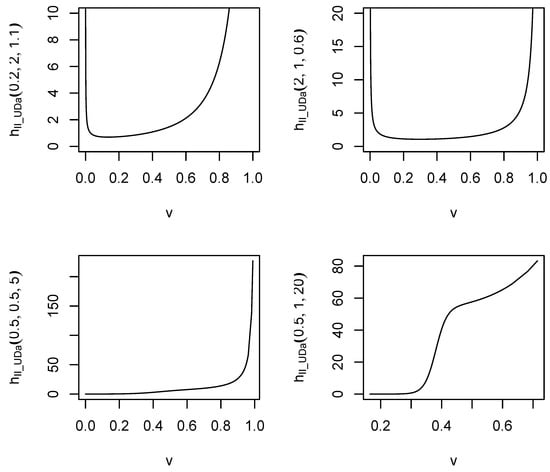
Figure 4. Hazard rate of II-UDa for different values of parameters.

It is easy to verify that a possible reparametrization of the type II unit-Dagum distribution in terms of the median and the $q-th$ quantile can be obtained as a solution of the following system:

$$\left\{\begin{array}{c}{\beta }_1=\frac{1}{\beta }\hfill \\ me=e^{-{\left[\frac{{0.5}^{-1/\beta }-1}{\lambda }\right]}^{-1/\delta }}\hfill \\ v\left(q\right)=e^{-{\left[\frac{{(1-q)}^{-1/\beta }-1}{\lambda }\right]}^{-1/\delta }}\hfill \end{array}\right.$$

(28)

that presents the following unique solution

$$\left\{\begin{array}{c}\beta =\frac{1}{{\beta }_1}\hfill \\ \lambda =\left[{0.5}^{-{\beta }_1}-1\right]·{\left[-log\left(me\right)\right]}^{\overline{\delta }}=\overline{\lambda }\hfill \\ \delta =\frac{log\left[{(1-q)}^{-{\beta }_1}-1\right]-log\left[{0.5}^{-{\beta }_1}-1\right]}{log\left[log\left(me\right)/log\left(v\right(q\left)\right)\right]}=\overline{\delta }\hfill \end{array}\right.$$

(29)

The corresponding distribution function is as follows:

$$\begin{array}{c}\hfill F_{R-II-UDa}(v;{\beta }_1,me,v\left(q\right))=1-{\left\{1+\overline{\lambda }{\left[-log\left(v\right)\right]}^{-\overline{\delta }}\right\}}^{-\frac{1}{{\beta }_1}}\end{array}$$

(30)

with ${\beta }_1>0$, $me\in (0,1)$ and $v\left(q\right)\in (0,1)$ for $q\in (0,1)$.

4. Inference

In this section, we use the maximum likelihood (ML) method to estimate the parameters of type I and type II unit-Dagum distributions under the hypothesis of homogeneity of the statistical units, i.e., assuming that there are no systematic factors (covariates), which make the observations heterogeneous. To this end, we first rewrite the probability density functions (14) and (23), in a single expression as follows

$$\begin{array}{ccc}& & f_{I-II-UDa}(v;\beta ,\lambda ,\delta )=\hfill \\ & & \beta \lambda \delta {\left[C^{-1}\left(v\right)\right]}^{-\delta -1}{\left\{1+\lambda {\left[C^{-1}\left(v\right)\right]}^{-\delta }\right\}}^{-\beta -1}\left\{-\frac{\partial C^{-1}\left(v\right)}{\partial v}\right\}\hfill \end{array}$$

(31)

where $C^{-1}\left(v\right)=log\frac{1+\sqrt{1-v^2}}{v}$ in the case of the type I unit-Dagum distribution or $C^{-1}\left(v\right)=-logv$ in the case of the type II unit-Dagum distribution. Let $\mathbf{v}=(v_1,\dots ,v_n)$ be a random sample of size n from (31), the log-likelihood function for $\mathit{\theta }=(\beta ,\lambda ,\delta )$ is as follows:

$$\begin{array}{ccc}\hfill {\ell }_{I-II-UDa}(\mathit{\theta };\mathbf{v})& \propto & nlog\left(\beta \lambda \delta \right)-(\delta +1){\displaystyle \sum _{i=1}^n}log{C}^{-1}\left(v_i\right)\hfill \\ & -& (\beta +1){\displaystyle \sum _{i=1}^n}log\left\{1+\lambda {\left[C^{-1}\left(v_i\right)\right]}^{-\delta }\right\}\hfill \end{array}$$

(32)

Differentiating ${\ell }_{I-II-UDa}(\mathit{\theta };\mathbf{v})$ with respect to $\beta$, $\lambda$, and $\delta$, respectively, we obtain the components of vector score $U\left(\mathit{\theta }\right)=(U_{\beta }\left(\mathit{\theta }\right),U_{\lambda }\left(\mathit{\theta }\right),U_{\delta }\left(\mathit{\theta }\right))$, where

$$\begin{array}{c}\hfill U_{\beta }\left(\mathit{\theta }\right)=\frac{\partial {\ell }_{I-II-UDa}(\mathit{\theta };\mathbf{v})}{\partial \beta }=\frac{n}{\beta }-{\displaystyle \sum _{i=1}^n}log\left\{1+\lambda {\left[C^{-1}\left(v_i\right)\right]}^{-\delta }\right\}\end{array}$$

(33)

$$\begin{array}{c}\hfill U_{\lambda }\left(\mathit{\theta }\right)=\frac{\partial {\ell }_{I-II-UDa}(\mathit{\theta };\mathbf{v})}{\partial \lambda }=\frac{n}{\lambda }-(\beta +1){\displaystyle \sum _{i=1}^n}\frac{{\left[C^{-1}\left(v_i\right)\right]}^{-\delta }}{1+\lambda {\left[C^{-1}\left(v_i\right)\right]}^{-\delta }}\end{array}$$

(34)

$$\begin{array}{ccc}\hfill U_{\delta }\left(\mathit{\theta }\right)& =& \frac{\partial {\ell }_{I-II-UDa}(\mathit{\theta };\mathbf{v})}{\partial \delta }=\frac{n}{\delta }-{\displaystyle \sum _{i=1}^n}log{C}^{-1}\left(v_i\right)\hfill \\ & +& (\beta +1)\frac{\lambda {\left[C\left(v_i\right)\right]}^{-\delta }log\left[C^{-1}\left(v_i\right)\right]}{1+\lambda {\left[C^{-1}\left(v_i\right)\right]}^{-\delta }}\hfill \end{array}$$

(35)

and setting the components of the score vector equal to zero, we obtain the system of likelihood equations, whose solution gives the ML estimates $\widehat{\mathit{\theta }}=(\widehat{\beta },\widehat{\lambda },\widehat{\delta })$ of the parameter vector $\mathit{\theta }=(\beta ,\lambda ,\delta )$. The system does not admit any explicit solution; therefore, the ML estimates $\widehat{\mathit{\theta }}$ can only be obtained by means of numerical procedures.

Confidence intervals and hypothesis tests for $\mathit{\theta }$ can be constructed using the usual asymptotic properties of the maximum likelihood estimators. In particular, we highlight that the expected Fisher information matrix of the parameter vector $\mathit{\theta }$ coincides with the expected Fisher information matrix of $\mathit{\theta }$ of the Dagum distribution (see Appendix A.3). This means that when constructing confidence intervals and hypothesis tests for the parameters of type I and II models of the unit-Dagum distribution, we can use the asymptotic variance and covariance matrix calculated in [32,33].

5. Unit-Dagum Regression Models

An important aspect to investigate is how heterogeneity among statistical units impacts possible measures of interest, such as median and extreme quantiles, simultaneously and directly. Given the particular nature of the dependent variable, this leads us to consider a regression approach where the response variable is defined on the unit interval.

The literature on this theme is wide and often deals with two different possibilities: properly transforming data to map the (0,1) interval to the real line and then using a common regression analysis, or choosing a suitable distribution and defining the relations among distribution parameters and covariates. Regarding the first kind of approach, various transformations are possible, and the logit is the most popular, but as [34] underlines, transformations can be inappropriate since the heteroscedasticity and skewness in data are not properly handled; moreover, the interpretation of results is possible only on the transformed scale. On the other hand, the second approach is nowadays preferred and widely explored, with different existing proposals based on various distributions and response variables. For example, when the attention is focused on the mean, the most popular distribution is the beta [35], but other possibilities are represented by simplex [36], log-Bilal [27], log-Lindley [37], log-weighted exponential [38], and unit gamma [39], to cite a few. When the focus is on the median or, in general, on the distribution quantiles, regression models can be based on Kumaraswamy [40], Johnson-t [41], log-extended exponential-geometric [42], L-logistic [43], or unit-type distributions (see, for example, [14,22,44]). Our proposal fits into the latter approach.

Specifically, given a sample of n observations, for each statistical unit i ($i=1,\dots ,n$), we observe the individual dependent variable value $v_i$ and the sets of individual covariates supposedly related to indicators and summarized in the vectors, ${\mathbf{x}}_{j,i}$, for $j=1,2,3$. The three sets of covariates ${\mathbf{x}}_{1,i}$, ${\mathbf{x}}_{2,i}$, and ${\mathbf{x}}_{3,i}$ are not necessarily the same, and, even if equal, their impact on the corresponding indicator may be different.

The vectors ${\mathbf{x}}_{ji}=(x_{ji1},x_{ji2},\dots ,x_{ji{p}_j})$ for $i=1,\dots ,n$, $j=1,2,3$, define the rows of three block $n\times p_j$ matrices ${\mathbf{X}}_j$ of $\mathbf{X}$. Each one refers to the $p_j$ covariates affecting the $j-th$ indicator $I_j$.

Each indicator, analogous to generalized linear models, is then related to the covariates, through an appropriate link function $h_j(·)$, as follows:

$$I_{j,i}=h_j({\mathbf{x}}_{j,i},{\gamma }_j).$$

(36)

The link functions are chosen to guarantee suitable restrictions on the parameter space, considering if $I_{j,i}$ is positive or varies on $(0,1)$. The elements of the vector ${\gamma }_j$$={({\gamma }_{j,1},{\gamma }_{j,2},\dots ,{\gamma }_{j,p_j})}^{\prime }$ are the unknown regression coefficients related to the $p_j$ individual characteristics to be estimated, applying the maximum likelihood method. By using the reformulation of unit-Dagum models in terms of indicators of interest, as shown in expressions (20) and (29), it is possible to relate the new parameters, such as the median and q-th quantile, to individual characteristics. In particular, observing that the solutions given in (20) and (29) are functions of the indicators of interest, i.e.,  ${\lambda }^{*}={\lambda }^{*}\left({\beta }_1,me,v\left(q\right)\right)$, ${\delta }^{*}={\delta }^{*}\left({\beta }_1,me,v\left(q\right)\right)$ for the type I unit-Dagum distribution and $\overline{\lambda }=\overline{\lambda }\left({\beta }_1,me,v\left(q\right)\right)$, $\overline{\delta }=\overline{\delta }\left({\beta }_1,me,v\left(q\right)\right)$ for the type II unit-Dagum distribution, and specifying the indicators of interest as functions of the covariates ${\beta }_{1,i}=h_1({\mathbf{x}}_{1,i},{\mathit{\gamma }}_1)$, $m{e}_i=h_2({\mathbf{x}}_{2,i},{\mathit{\gamma }}_2)$ and $v{\left(q\right)}_i=h_3({\mathbf{x}}_{3,i},{\mathit{\gamma }}_3)$, from  (21) and (30), for the i-th observation, we can rewrite the pdfs as functions of the regression coefficients ${\mathit{\gamma }}_1$, ${\mathit{\gamma }}_2$, and ${\mathit{\gamma }}_3$. Similar to what was done previously, we use a single structure to represent type I and type II unit-Dagum distributions, simultaneously, as follows:

$$\begin{array}{ccc}\hfill f_{R-I-II-UDa}(v_i;{\mathit{\gamma }}_1,{\mathit{\gamma }}_2,{\mathit{\gamma }}_3)& =& \frac{{\tilde{\lambda }}_i{\tilde{\delta }}_i}{{\tilde{\beta }}_{1,i}}{\left[C^{-1}\left(v\right)\right]}^{-{\tilde{\delta }}_i-1}{\left\{1+{\tilde{\lambda }}_i{\left[C^{-1}\left(v\right)\right]}^{-{\tilde{\delta }}_i}\right\}}^{-\frac{1}{{\tilde{\beta }}_{1,i}}-1}\hfill \\ & \times & \left\{-\frac{\partial C^{-1}\left(v\right)}{\partial v_i}\right\}\hfill \end{array}$$

(37)

where ${\tilde{\lambda }}_i={\lambda }_i^{*}$, ${\tilde{\delta }}_i={\delta }_i^{*}$ in the case of the type I unit-Dagum, and ${\tilde{\lambda }}_i={\overline{\lambda }}_i$, ${\tilde{\delta }}_i={\overline{\delta }}_i$ in the type II unit-Dagum distribution. Putting $\gamma ={({\gamma }_1^{{}^{\prime }},{\gamma }_2^{{}^{\prime }},{\gamma }_3^{{}^{\prime }})}^{{}^{\prime }}$, by (37), the i-th element of the log-likelihood function is

$$\begin{array}{ccc}\hfill \ell (\mathit{\gamma };\mathbf{v},\mathbf{X})& \propto & log\left({\tilde{\lambda }}_i\right)+log\left({\tilde{\delta }}_i\right)-log\left({\tilde{\beta }}_{1,i}\right)-({\tilde{\delta }}_i+1)log\left[C^{-1}\left(v_i\right)\right]\hfill \\ & -& \left(\frac{1}{{\tilde{\beta }}_{1,i}}+1\right)log\left(1+{\tilde{\lambda }}_i{\left[C^{-1}\left(v_i\right)\right]}^{-{\tilde{\delta }}_i}\right).\hfill \end{array}$$

(38)

Remembering that the parameters ${\tilde{\beta }}_{1,i}$, ${\tilde{\lambda }}_i$, and ${\tilde{\delta }}_i$ are functions of the vector $\mathit{\gamma }$ of the dimension $p=p_1+p_2+p_3$, the $j{r}_j-th$ equation of the likelihood system is given by

$$\begin{array}{ccc}\hfill \frac{\partial \ell (\gamma ;\mathbf{v},\mathbf{X})}{\partial {\gamma }_{j,r_j}}& =& \frac{1}{{\tilde{\lambda }}_i}\left(\frac{\partial {\tilde{\lambda }}_i}{\partial {\gamma }_{j,r_j}}\right)+\frac{1}{{\tilde{\delta }}_i}\left(\frac{\partial {\tilde{\delta }}_i}{\partial {\gamma }_{j,r_j}}\right)-\frac{1}{{\tilde{\beta }}_{1,i}}\left(\frac{\partial {\tilde{\beta }}_{1,i}}{\partial {\gamma }_{j,r_j}}\right)\hfill \\ & -& log\left[C^{-1}\left(v_i\right)\right]\left(\frac{\partial {\tilde{\delta }}_i}{\partial {\gamma }_{j,r_j}}\right)+\frac{1}{{\left({\tilde{\beta }}_{1,i}\right)}^2}\left(\frac{\partial {\tilde{\beta }}_{1,i}}{\partial {\gamma }_{j,r_j}}\right)log\left(1+{\tilde{\lambda }}_i{\left[C^{-1}\left(v_i\right)\right]}^{-{\tilde{\delta }}_i}\right)\hfill \\ & -& \left(\frac{1}{{\tilde{\beta }}_{1,i}}+1\right)\frac{\left(\frac{\partial {\tilde{\lambda }}_i}{\partial {\gamma }_{j,r_j}}\right)-{\tilde{\lambda }}_i\left(\frac{\partial {\tilde{\delta }}_i}{\partial {\gamma }_{j,r_j}}\right)log\left[C^{-1}\left(v_i\right)\right]}{{\left[C^{-1}\left(v_i\right)\right]}^{{\tilde{\delta }}_i}+{\tilde{\lambda }}_i}=0\hfill \end{array}$$

(39)

for $j=1,2,3$ and $r_j=1,2,\dots ,p_j$. The partial derivatives in system (39) are given in Appendix A.4.

The system of the likelihood equations does not admit any explicit solution; therefore, the ML estimates ${\widehat{\gamma }}_{j,r_j}$ for $j=1,2,3$ and $r_j=1,2,\dots ,p_j$ can only be obtained by means of numerical procedures. Under the usual regularity conditions, the known asymptotic properties of the maximum likelihood method ensure that $\sqrt{(}n)({\widehat{\mathit{\gamma }}}_n-\mathit{\gamma })\stackrel{d}{\to }N(\mathbf{0},{\Sigma }_{\mathit{\gamma }})$, where ${\Sigma }_{\mathit{\gamma }}={[{lim}_{n\to \infty }\mathbf{I}\left(\mathit{\gamma }\right)/n]}^{-1}$ is the $(p_1+p_2+p_3)\times (p_1+p_2+p_3)$ asymptotic variance–covariance matrix and $\mathbf{I}\left(\mathit{\gamma }\right)$ is the Fisher information matrix, given by $\mathbf{I}\left(\mathit{\gamma }\right)=-E\left(\mathbf{H}\right)$, where $\mathbf{H}$ is the Hessian matrix of the second partial derivatives of the log-likelihood function, i.e.,$\frac{{\partial }^2\ell (\mathit{\gamma };\mathbf{v},\mathbf{X})}{\partial {\gamma }_{j,r_j}{\gamma }_{h,r_h}}$. Elements of the $\mathbf{I}\left(\mathit{\gamma }\right)$ matrix are not reported here for space purposes, but are available upon request.

6. Applications

In order to show the potentiality of the proposed models, we consider two famous and widely used datasets, referred to data that fall into the unit interval and contained in the R package, betareg, namely household food expenditures and reading skills. In particular, the household food expenditure data regard the proportion of income spent on food for 38 households living in a large U.S. city and contain information on the perceived income and the number of persons living in the household. The reading skills dataset refers to the scores obtained in a test on reading accuracy involving 44 Australian children, including 19 dyslexic subjects and 25 non-dyslexic subjects. Moreover, the status of each child, and information regarding the nonverbal intelligent quotient (iq), are available.

These datasets were used by [34] to describe the implementation of the beta regression in the R system and to underline the advantage of this kind of regression with respect to the linear one when data belong to the unit interval. Therefore, as a further aim of this section, we will compare the performance of the unit-Dagum regression models with that of the widely used beta regression. Indeed, both methodologies give us the possibility to evaluate, among other aspects, the impact of some covariates on measures of central tendency, namely the mean in the case of the beta regression, and the median in the case of the unit-Dagum regression. It is worth noting that when data exhibit skewness, the median should be preferred as the centrality measure. Therefore, the proposed regression could be more appropriate in some cases.

6.1. Modeling Food/Income and Accuracy Data

In this section, we consider the proportion of income spent on food and the scores regarding reading accuracy. The corresponding empirical distributions are shown in Figure 5. To evaluate the adequacy of the proposed models in describing the considered data, the maximum likelihood estimates (MLEs) of the parameters for the I-UDa and II-Da densities reported in (14) and (23) are obtained, along with the corresponding standard errors and the values for the Akaike information criterion (AIC). Moreover, we compare the obtained results with the analogs for the beta and Kumuraswamy (KW) models, which are likely the most used models for data on bounded support. Table 2 presents the obtained results. Both the AIC values and the inspection of Figure 5 suggest that the proposed models better describe the considered data if compared with the beta and KW distributions. In particular, the lower value of the AIC for food expenditure data is obtained in correspondence with the type II unit-Dagum model, while, for reading skills data, the type I unit-Dagum reaches the lower result, far from the beta and KW ones. We should note that the chosen data are very different from each other in terms of the distribution shape, so these examples give us the possibility of testing the flexibilities of our models and their ability to properly reproduce different characteristics of the phenomena, such as unimodality, increasing density, presence of asymmetry, fat tails, and so on.

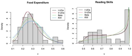
Figure 5. Empirical and fitted distributions for I-Da, II-Da, beta, and KW models.

Table 2. MLEs, corresponding standard errors (in brackets), and AIC values for I-Da, II-Da, beta, and KW models in food expenditure and reading skills data.

	I-UDa	II-UDa	Beta	KW
	Food Expenditures
$\beta$	0.484 (1.618)	0.410 (1.631)	6.070 (1.358)	2.954 (0.309)
$\lambda$	30,279.37 (34.380)	62.520 (6.985)	14.819 (3.398)	26.964 (8.700)
$\delta$	13.457 (1.326)	10.056 (1.360)
AIC	−67.337	−67.400	−66.693	−62.978
	Reading Skills
$\beta$	0.044 (1.661)	0.038 (1.670)	2.514 (0.578)	2.694 (0.589)
$\lambda$	529.384 (29.316)	0.004 (15.152)	0.675 (0.123)	0.665 (0.121)
$\delta$	24.287 (1.604)	14.917 (1.617)
AIC	−65.366	−64.134	−48.841	−49.218

6.2. Considering the Covariates: The Regression Models

In this section, we consider both type I and type II unit-Dagum distributions according to a regressive perspective and we compare their performances with results from the well-known beta regression.

To this end, we also take into account data regarding covariates and results reported in [34], corresponding with the best beta regression model for each dataset. We should note that, as can be viewed from Figure 5, both the income/food proportions and the reading accuracy scores show an asymmetric distribution; therefore, attention is placed on the median rather than the mean of the distribution, and it could be more appropriate to analyze the central tendency.

Food expenditure data

For the first dataset, information on household income and the number of people living in the household are available. Starting with the reparameterization data reported in (19) and (28), we consider the effect of these covariates on the median and 90th quantile, according to the regression models described in Section 5. Since both the indicators assume values in the unit interval, a logit-link function is used to relate the median and 90th quantiles to the covariates. Moreover, we consider an intercept term related to the ${\beta }_1$ indicator through a log-link function, which is suitable for positive indicators. The ML estimates of the coefficients, their standard errors, and results from the Wald test are reported in Table 3. In both models, we find that the median and 90th quantiles of the proportions spent on food decrease as income increases, while the number of persons living in a household shows a positive significant effect on the 90th quantile, ceteris paribus. Moreover, both models outperformed the beta regression in terms of AIC (−88.37 for beta regression), with the best results obtained for II-UDa regression. A comparison between empirical and fitted curves reported in Figure 6 confirms these results. In particular, here, two different curves are shown for each model. Indeed, through the regression approach and the resulting estimates, it is possible to consider the behaviors of density functions for different covariate values. The depicted curves refer to the median and $v\left(0.9\right)$ indicators for the I-Da and II-Da model, and to the mean and dispersion parameters for the beta model, when income and the number of persons are equal to the average level observed for $v\le 0.5$ and $v>0.5$, respectively (${\mu }_{inc}=60.65$; ${\mu }_{pers}=3.37$ vs. ${\mu }_{inc}=32.65$; ${\mu }_{pers}=6$). This allows us to evaluate the ability of the models to describe the right distribution tail, as well as the central tendency.

Table 3. MLEs, corresponding standard errors, and Wald test results for the I-Da and II-Da regression models for food expenditure data.

	I-UDa
	Estimate	SE	z	p-Value
	$I_1={\beta }_1$ (log-link)
Intercept	−0.333	0.506	−0.659	0.51
	$I_2=me$ (logit-link)
Intercept	−0.544	0.016	−33.974	$<0.001$
income	−0.009	0.001	−16.758	$<0.001$
	$I_3=v\left(0.9\right)$ (logit-link)
Intercept	−0.727	0.022	−33.362	$<0.001$
income	−0.008	0.000	−21.604	$<0.001$
persons	0.167	0.022	7.425	$<0.001$
	AIC = −92.29
	II-UDa
	Estimate	SE	z	p-Value
	$I_1={\beta }_1$ (log-link)
Intercept	−3.672	4.586	−0.801	0.423
	$I_2=me$ (logit-link)
Intercept	−0.552	0.015	−36.371	$<0.001$
income	−0.009	0.000	−18.971	$<0.001$
	$I_3=v\left(0.9\right)$ (logit-link)
Intercept	−0.724	0.014	−50.203	$<0.001$
income	−0.008	0.000	−25.635	$<0.001$
persons	0.160	0.015	10.351	$<0.001$
	AIC = −97.25

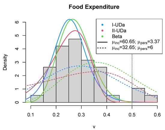
Figure 6. Empirical and fitted distributions for I-Da, II-Da, and beta models. The solid lines and the dotted lines refer to the average values of covariates obtained, respectively, for $v\le 0.5$ and $v>0.5$.

Reading skills data

In the reading skills dataset, in addition to information regarding the presence of dyslexia, z scores for the nonverbal intelligent quotient (iq) test are available. Therefore, we can consider the effects of these characteristics on the median and 90th quantiles of reading accuracy scores, by specifying a logit-link function to relate indicators and covariates. In particular, as suggested by [34], we consider an interaction term between iq and dyslexia. Once again, we relate an intercept term to ${\beta }_1$, using a log-link function. Similar to that obtained by [34] for regression on the mean indicator, we find a significant main and interaction effect on the median for dyslexia and iq, for both I-Da and II-Da models. Specifically, results reported in Table 4 confirm the positive effect of iq and the negative effect for dyslexia and the interaction term. Moreover, we also find a significant negative effect of dyslexia on the 90th quantile.

Table 4. MLEs, corresponding standard errors, and Wald test results for the I-Da and II-Da regression models for reading skills data.

	I-UDa
	Estimate	SE	z	p-Value
	$I_1={\beta }_1$ (log-link)
Intercept	−0.9626	0.9008	−1.069	0.285
	$I_2=me$ (logit-link)
Intercept	1.593	0.175	9.107	$<0.001$
dyslexia	−1.119	0.167	−6.707	$<0.001$
iq	0.504	0.093	5.389	$<0.001$
dyslexia × iq	−0.512	0.094	−5.451	$<0.001$
	$I_3=v\left(0.9\right)$ (logit-link)
Intercept	2.69045	0.03643	73.85	$<0.001$
Dyslexia	−1.914	0.03643	−52.544	$<0.001$
	AIC = −139.32
	II-UDa
	Estimate	SE	z	p-Value
	$I_1={\beta }_1$ (log-link)
Intercept	−0.7247	0.80705	−0.898	0.369
	$I_2=me$ (logit-link)
Intercept	1.60156	0.18082	8.857	$<0.001$
dyslexia	−1.1376	0.17224	−6.605	$<0.001$
iq	0.49774	0.09663	5.151	$<0.001$
dyslexia × iq	−0.5047	0.09701	−5.202	$<0.001$
	$I_3=v\left(0.9\right)$ (logit-link)
Intercept	2.69356	0.03759	71.648	$<0.001$
dyslexia	−1.9168	0.03768	−50.873	$<0.001$
	AIC = −137.41

In this case, the model with the best performance in terms of AIC is the I-Da one, but both of the proposed models show lower values than the beta regression (AIC = −117.8). Figure 7 shows the comparisons among empirical and fitted distributions for dyslexic and non-dyslexic subjects, considering an average iq level that is equal to −0.653 for dyslexic subjects and 0.4966 for control subjects.

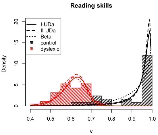
Figure 7. Empirical and fitted distributions for I-Da, II-Da, and beta models. Different curves refer to dyslexic and non-dyslexic subjects, considering the average iq level for each group.

7. Concluding Remarks

In this paper, we show that many of the existing proposals on probability distributions for data in the unit interval can be viewed as particular cases of a general class of models, obtained using the techniques of rv transformations. In the present paper, expressions on the distribution and density functions of the class are given and the principal characteristics are furnished. Through the proper transformation choice, it is possible to obtain new distribution functions on bounded support, whose characteristics are easy to derive. Indeed, two new distributions are proposed, starting with the Dagum model, and considering two different transformations. The resulting models are particularly flexible, as is evident by choosing different sets of parameter values and by looking at the behavior of their densities and hazard functions.

We also considered the possibility of reparameterizing the distributions in order to express them in terms of the indicators of interest. In particular, we obtained models that depend on the median and quantile; this gave us the opportunity to relate these quantities to covariates, according to a regressive perspective. Given the particular nature of the involved variables, this led us to consider the regression approach, where the response variable was defined on the unit interval. Therefore, the proposed methodology can be considered as an alternative to other approaches that are often employed when the response variable represents proportions, rates, or percentages. Furthermore, considering regression on the median could be more appropriate in the presence of asymmetry. The applications on two different datasets allowed us to evaluate the behaviors of the suggested models and compare their performances with the most widely used approach in this context, namely the beta regression. The obtained findings are encouraging since both models seem to be very competitive.

Appendix A.1. Proof of Proposition 1

First, in the following expression

$$\begin{array}{ccc}\hfill E\left[V^r\right]& =& {\int }_0^1{v}^r\frac{\beta \lambda \delta }{v\sqrt{1-v^2}}{\left[log\left(\frac{1+\sqrt{1-v^2}}{v}\right)\right]}^{-\delta -1}\hfill \\ & & {\left\{1+\lambda {\left[log\left(\frac{1+\sqrt{1-v^2}}{v}\right)\right]}^{-\delta }\right\}}^{-\beta -1}dv\hfill \end{array}$$

putting $z={\left\{1+\lambda {\left[log\left(\frac{1+\sqrt{1-v^2}}{v}\right)\right]}^{-\delta }\right\}}^{-1}$, with $dv=-\frac{v\sqrt{1-v^2}}{\lambda \delta }{\left[log\left(\frac{1+\sqrt{1-v^2}}{v}\right)\right]}^{\delta +1}{\left\{1+\lambda {\left[log\left(\frac{1+\sqrt{1-v^2}}{v}\right)\right]}^{-\delta }\right\}}^{2}dz$, after algebra, we obtain

$$\begin{array}{c}\hfill E\left[V^r\right]=\beta {\int }_0^1{\left(2e^{{\lambda }^{\frac{1}{\delta }}{\left(\frac{z}{1-z}\right)}^{\frac{1}{\delta }}}\right)}^r{\left(1+e^{2{\lambda }^{\frac{1}{\delta }}{\left(\frac{z}{1-z}\right)}^{\frac{1}{\delta }}}\right)}^{-r}{z}^{\beta -1}dz.\end{array}$$

Now, using Newton’s Binomial theorem, we can write

$$\begin{array}{c}\hfill {\left(\frac{2e^{{\lambda }^{\frac{1}{\delta }}{\left(\frac{z}{1-z}\right)}^{\frac{1}{\delta }}}}{1+e^{2{\lambda }^{\frac{1}{\delta }}{\left(\frac{z}{1-z}\right)}^{\frac{1}{\delta }}}}\right)}^r=2^r\frac{e^{-r{\lambda }^{\frac{1}{\delta }}{\left(\frac{z}{1-z}\right)}^{\frac{1}{\delta }}}}{{\left(1+e^{-2{\lambda }^{\frac{1}{\delta }}{\left(\frac{z}{1-z}\right)}^{\frac{1}{\delta }}}\right)}^r}=2^r{\displaystyle \sum _{j=0}^{+\infty }}\left(\genfrac{}{}{0pt}{}{-r}{j}\right)e^{-(2j+r){\lambda }^{\frac{1}{\delta }}{\left(\frac{z}{1-z}\right)}^{\frac{1}{\delta }}}\end{array}$$

substituting this last result in the rth moment, we obtain

$$\begin{array}{c}\hfill E\left[V^r\right]=\beta 2^r{\displaystyle \sum _{j=0}^{+\infty }}\left(\genfrac{}{}{0pt}{}{-r}{j}\right){\int }_0^1{e}^{-(2j+r){\lambda }^{\frac{1}{\delta }}{\left(\frac{z}{1-z}\right)}^{\frac{1}{\delta }}}{z}^{\beta -1}dz\end{array}$$

Putting $y=(2j+r){\lambda }^{\frac{1}{\delta }}{\left(\frac{z}{1-z}\right)}^{\frac{1}{\delta }}$, with $y\in (0,\infty )$ and $dz=\delta {(2j+r)}^{\frac{1}{\delta }}\lambda y^{\delta -1}{[(2j+r)}^{\frac{1}{\delta }}\lambda +$$y^{\delta }{]}^{-2}dy$, after algebra, we obtain

$$\begin{array}{ccc}\hfill E\left[V^r\right]& =& \beta 2^r{\displaystyle \sum _{j=0}^{+\infty }}\left(\genfrac{}{}{0pt}{}{-r}{j}\right)\frac{1}{\beta }{\int }_0^{+\infty }{e}^{-y}\beta \delta {(2j+r)}^{\frac{1}{\delta }}\lambda y-\delta -1{\left(1+{(2j+r)}^{\frac{1}{\delta }}\lambda y^{-\delta }\right)}^{-\beta -1}dy\hfill \\ & =& 2^r{\displaystyle \sum _{j=0}^{+\infty }}\left(\genfrac{}{}{0pt}{}{-r}{j}\right)E\left[e^{-Y};\beta ,\delta ,\lambda {(2j+r)}^{\frac{1}{\delta }}\right]\hfill \\ & =& \beta 2^r{\displaystyle \sum _{j=0}^{+\infty }}\left(\genfrac{}{}{0pt}{}{-r}{j}\right){\displaystyle \sum _{s=0}^{+\infty }}\frac{{(-1)}^s}{s!}{\lambda }^{\frac{s}{\delta }}{(2j+r)}^{s}B\left(\beta +\frac{s}{\delta },1-\frac{s}{\delta }\right).\hfill \end{array}$$

Appendix A.2. Proof of Proposition 2

Given the considered transformation $V:=C\left(Y\right)=e^{-Y}$, it is evident that the r-th moment of the type II unit-Dagum distribution coincides with the Laplace transform of the Dagum distribution, i.e.,

$$\begin{array}{ccc}\hfill E\left[V^r\right]& =& E\left[e^{-rY}\right]\hfill \\ & =& \beta \lambda \delta {\int }_0^{+\infty }{e}^{-rt}{t}^{-\delta -1}{(1+\lambda t^{-\delta })}^{-\beta -1}dt\hfill \end{array}$$

and putting $e^{-rt}={\sum }_{s=0}^{+\infty }\frac{{(-rt)}^s}{s!}$, we obtain:

$$\begin{array}{ccc}\hfill E\left[V^r\right]& =& {\displaystyle \sum _{s=0}^{+\infty }}\frac{{(-r)}^s}{s!}{\int }_0^{+\infty }{t}^s\beta \lambda \delta t^{-\delta -1}{(1+\lambda t^{-\delta })}^{-\beta -1}dt\hfill \\ & =& {\displaystyle \sum _{s=0}^{+\infty }}\frac{{(-r)}^s}{s!}{\mu }_{Da}^s.\hfill \end{array}$$

Substituting expression (12) into the s-th moment of the Dagum distribution in the previous equation, we obtain the expression for the r-th moment of the type II unit-Dagum distribution.

Appendix A.3. Fisher Information Matrix

In order to compute the expected Fisher information matrix, we consider the following elements of the Hessian matrix:

$$\begin{array}{c}\hfill \frac{{\partial }^2{\ell }_{I-II-UDa}(\mathit{\theta };\mathbf{v})}{\partial {\beta }^2}=-\frac{n}{{\beta }^2}\end{array}$$

(A1)

$$\begin{array}{c}\hfill \frac{{\partial }^2{\ell }_{I-II-UDa}(\mathit{\theta };\mathbf{v})}{\partial \beta \lambda }=-{\displaystyle \sum _{i=1}^n}\frac{{\left[C^{-1}\left(v_i\right)\right]}^{-\delta }}{1+\lambda {\left[C^{-1}\left(v_i\right)\right]}^{-\delta }}\end{array}$$

(A2)

$$\begin{array}{c}\hfill \frac{{\partial }^2{\ell }_{I-II-UDa}(\mathit{\theta };\mathbf{v})}{\partial \beta \delta }={\displaystyle \sum _{i=1}^n}\frac{\lambda {\left[C^{-1}\left(v_i\right)\right]}^{-\delta }ln\left[C^{-1}\left(v_i\right)\right]}{1+\lambda {\left[C^{-1}\left(v_i\right)\right]}^{-\delta }}\end{array}$$

(A3)

$$\begin{array}{c}\hfill \frac{{\partial }^2{\ell }_{I-II-UDa}(\mathit{\theta };\mathbf{v})}{\partial {\lambda }^2}=-\frac{n}{{\lambda }^2}+(\beta +1){\displaystyle \sum _{i=1}^n}\frac{{\left[C^{-1}\left(v_i\right)\right]}^{-2\delta }}{{\left\{1+\lambda {\left[C^{-1}\left(v_i\right)\right]}^{-\delta }\right\}}^2}\end{array}$$

(A4)

$$\begin{array}{c}\hfill \frac{{\partial }^2{\ell }_{I-II-UDa}(\mathit{\theta };\mathbf{v})}{\partial \lambda \delta }=(\beta +1){\displaystyle \sum _{i=1}^n}\frac{{\left[C^{-1}\left(v_i\right)\right]}^{-\delta }ln\left[C^{-1}\left(v_i\right)\right]}{{\left\{1+\lambda {\left[C^{-1}\left(v_i\right)\right]}^{-\delta }\right\}}^2}\end{array}$$

(A5)

$$\begin{array}{c}\hfill \frac{{\partial }^2{\ell }_{I-II-UDa}(\mathit{\theta };\mathbf{v})}{\partial {\delta }^2}=-\frac{n}{{\delta }^2}-\lambda (\beta +1){\displaystyle \sum _{i=1}^n}\frac{{\left[C^{-1}\left(v_i\right)\right]}^{-\delta }{\left\{ln\left[C^{-1}\left(v_i\right)\right]\right\}}^2}{{\left\{1+\lambda {\left[C^{-1}\left(v_i\right)\right]}^{-\delta }\right\}}^2}.\end{array}$$

(A6)

The elements of the expected Fisher information matrix are functions of the following expectation, with respect to the density function of the rv V

$$\begin{array}{c}\hfill E_{j_1,j_2,j_3}=E_V\left\{\frac{{\left[C^{-1}\left(V\right)\right]}^{-j_1\delta }{\left(ln\left[C^{-1}\left(V\right)\right]\right)}^{j_2}}{{\left(1+\lambda {\left[C^{-1}\left(V\right)\right]}^{-\delta }\right)}^{j_3}}\right\}\end{array}$$

(A7)

We now observe that for a generic function $h(.)$ of $C^{-1}\left(V\right)$, by a simple transformation of the variable, we can write

$$\begin{array}{ccc}\hfill E_V\left\{h\left[C^{-1}\left(V\right)\right]\right\}& =& {\int }_0^{1}h\left[C^{-1}\left(v\right)\right]f_V(v;\mathit{\theta })dv=\hfill \\ & =& {\int }_0^{1}h\left[C^{-1}\left(v\right)\right]\beta \lambda \delta {\left[C^{-1}\left(v\right)\right]}^{-\delta -1}{\left\{1+\lambda {\left[C^{-1}\left(v\right)\right]}^{-\delta }\right\}}^{-\beta -1}\left[-\frac{\partial C^{-1}\left(v\right)}{\partial v}\right]dv=\hfill \\ & =& {\int }_0^{\infty }h\left[y\right]\beta \lambda \delta {\left[y\right]}^{-\delta -1}{\left\{1+\lambda {\left[y\right]}^{-\delta }\right\}}^{-\beta -1}dy=E_Y\left[h\left(Y\right)\right]\hfill \end{array}$$

where $Y\sim Da(\beta ,\lambda ,\delta )$. Using this last observation, Equation (A7) can be rewritten as

$$\begin{array}{ccc}\hfill E_{j_1,j_2,j_3}& =& E_Y\left\{\frac{{\left[Y\right]}^{-j_1\delta }{\left(ln\left[Y\right]\right)}^{j_2}}{{\left(1+\lambda {\left[Y\right]}^{-\delta }\right)}^{j_3}}\right\}\hfill \\ & =& {\int }_0^{\infty }\frac{y^{-j_1\delta }{\left(ln\left(y\right)\right)}^{j_2}}{{\left(1+\lambda y^{-\delta }\right)}^{j_3}}\beta \lambda \delta y^{-\delta -1}{\left(1+\lambda y^{-\delta }\right)}^{-\beta -1}dy\hfill \\ & =& \frac{\beta }{{\lambda }^{j_1}{\delta }^{j_2}}{\int }_0^1{y}^{\beta -j_1+j_3-1}{(1-y)}^{\frac{2}{\delta }+j_1}{\left[ln\left(\lambda \right)+ln\left(y\right)-ln(1-y)\right]}^{j_2}dy\hfill \end{array}$$

(A8)

Using the successive derivatives of the beta function, the expectations for determining the elements of the Fisher information matrix are

$$\begin{array}{c}\hfill E_{1,0,1}=\frac{\beta }{\lambda }B(\beta ,2+\frac{2}{\delta })\end{array}$$

(A9)

$$\begin{array}{c}\hfill E_{2,0,2}=\frac{\beta }{{\lambda }^2}B(\beta ,3+\frac{2}{\delta })\end{array}$$

(A10)

$$\begin{array}{c}\hfill E_{1,1,1}=\frac{\beta }{\lambda \delta }\left\{ln\left(\lambda \right)B(\beta ,2+\frac{2}{\delta })+A_1(\beta ,2+\frac{2}{\lambda \delta })+A_2(\beta +1,2+\frac{2}{\delta })\right\}\end{array}$$

(A11)

$$\begin{array}{c}\hfill E_{1,1,2}=\frac{\beta }{\lambda \delta }\left\{ln\left(\lambda \right)B(\beta +1,2+\frac{2}{\delta })+A_1(\beta ,3+\frac{2}{\lambda \delta })+A_2(\beta +1,2+\frac{2}{\delta })\right\}\end{array}$$

(A12)

$$\begin{array}{ccc}\hfill E_{1,2,2}& =& \frac{\beta }{\lambda {\delta }^2}\left\{{[ln\left(\lambda \right)]}^{2}B(\beta +1,2+\frac{2}{\delta })+2ln\left(\lambda \right)A_1(\beta +1,2+\frac{2}{\lambda \delta })-2ln\left(\lambda \right)A_2(\beta +1,2+\frac{2}{\delta })\right.\hfill \\ & +& \left.A_3(\beta +1,2+\frac{2}{\delta })-2A_5(\beta +1,2+\frac{2}{\delta })+A_4(\beta +1,2+\frac{2}{\delta })\right\}\hfill \end{array}$$

(A13)

where

$$\begin{array}{c}\hfill A_1(p,q)=B(p,q)\left\{\psi \left(p\right)-\psi (p+q)\right\}\end{array}$$

$$\begin{array}{c}\hfill A_2(p,q)=B(p,q)\left\{\psi \left(q\right)-\psi (p+q)\right\}\end{array}$$

$$\begin{array}{c}\hfill A_3(p,q)=B(p,q)\left\{{[\psi \left(p\right)-\psi (p+q)]}^2+[{\psi }^{{}^{\prime }}\left(p\right)-{\psi }^{{}^{\prime }}(p+q)]\right\}\end{array}$$

$$\begin{array}{c}\hfill A_4(p,q)=B(p,q)\left\{{[\psi \left(q\right)-\psi (p+q)]}^2+[{\psi }^{{}^{\prime }}\left(q\right)-{\psi }^{{}^{\prime }}(p+q)]\right\}\end{array}$$

$$\begin{array}{c}\hfill A_5(p,q)=B(p,q)\left\{[\psi \left(q\right)-\psi (p+q)][\psi \left(p\right)-\psi (p+q)]+[{\psi }^{{}^{\prime }}\left(p\right)-{\psi }^{{}^{\prime }}(p+q)]\right\}\end{array}$$

with $\psi (.)$ and ${\psi }^{{}^{\prime }}(.)$ being digamma and trigamma functions, respectively.

In order to compute the expected Fisher information matrix, we compute the elements of the Hessian matrix, which, after some algebraic manipulation, for $j,s=1,2,3$ and $r_j=1,2,\dots ,p_j$ and $r_s=1,2,\dots ,p_s$, turn out to be

$$\begin{array}{ccc}\hfill \frac{{\partial }^2\ell (\mathit{\gamma };\mathbf{v},\mathbf{X})}{\partial {\gamma }_{j,r_j}\partial {\gamma }_{s,r_s}}& =& k_1+k_2-k_3+k_{4}ln\left(1+{\tilde{\lambda }}_i{\left[C^{-1}\left(v_i\right)\right]}^{-{\tilde{\delta }}_i}\right)+k_6\frac{{\left[C^{-1}\left(v_i\right)\right]}^{-{\tilde{\delta }}_i}}{1+{\tilde{\lambda }}_i{\left[C^{-1}\left(v_i\right)\right]}^{-{\tilde{\delta }}_i}}\hfill \\ & +& k_7\frac{{\left[C^{-1}\left(v_i\right)\right]}^{-{\tilde{\delta }}_i}ln\left[C^{-1}\left(v_i\right)\right]}{1+{\tilde{\lambda }}_i{\left[C^{-1}\left(v_i\right)\right]}^{-{\tilde{\delta }}_i}}+\left(\frac{1}{{\tilde{\beta }}_{1,i}}+1\right)\hfill \\ & \times & \left\{\left(\frac{\partial {\tilde{\lambda }}_i}{\partial {\gamma }_{j,r_j}}\right)\left(\frac{\partial {\tilde{\delta }}_i}{\partial {\gamma }_{s,r_s}}\right)\frac{{\left[C^{-1}\left(v_i\right)\right]}^{-{\tilde{\delta }}_i}\left(ln\left[C^{-1}\left(v_i\right)\right]\right)}{{\left(1+{\tilde{\lambda }}_i{\left[C^{-1}\left(v_i\right)\right]}^{-{\tilde{\delta }}_i}\right)}^2}\right.\hfill \\ & +& \left(\frac{\partial {\tilde{\lambda }}_i}{\partial {\gamma }_{j,r_j}}\right)\left(\frac{\partial {\tilde{\lambda }}_i}{\partial {\gamma }_{s,r_s}}\right)\frac{{\left[C^{-1}\left(v_i\right)\right]}^{-2{\tilde{\delta }}_i}}{{\left(1+{\tilde{\lambda }}_i{\left[C^{-1}\left(v_i\right)\right]}^{-{\tilde{\delta }}_i}\right)}^2}\hfill \\ & -& {\tilde{\lambda }}_i\left(\frac{\partial {\tilde{\delta }}_i}{\partial {\gamma }_{j,r_j}}\right)\left(\frac{\partial {\tilde{\delta }}_i}{\partial {\gamma }_{s,r_s}}\right)\frac{{\left[C^{-1}\left(v_i\right)\right]}^{-{\tilde{\delta }}_i}{\left(ln\left[C^{-1}\left(v_i\right)\right]\right)}^2}{{\left(1+{\tilde{\lambda }}_i{\left[C^{-1}\left(v_i\right)\right]}^{-{\tilde{\delta }}_i}\right)}^2}\hfill \\ & -& \left.{\tilde{\lambda }}_i\left(\frac{\partial {\tilde{\delta }}_i}{\partial {\gamma }_{j,r_j}}\right)\left(\frac{\partial {\tilde{\lambda }}_i}{\partial {\gamma }_{s,r_s}}\right)\frac{{\left[C^{-1}\left(v_i\right)\right]}^{-2{\tilde{\delta }}_i}\left(ln\left[C^{-1}\left(v_i\right)\right]\right)}{{\left(1+{\tilde{\lambda }}_i{\left[C^{-1}\left(v_i\right)\right]}^{-{\tilde{\delta }}_i}\right)}^2}\right\}\hfill \end{array}$$

(A14)

where

$k_1=\frac{1}{{\tilde{\lambda }}_i}\left[-\frac{1}{{\tilde{\lambda }}_i}\left(\frac{\partial {\tilde{\lambda }}_i}{\partial {\gamma }_{s,r_s}}\right)\left(\frac{\partial {\tilde{\lambda }}_i}{\partial {\gamma }_{j,r_j}}\right)+\left(\frac{{\partial }^2{\tilde{\lambda }}_i}{\partial {\gamma }_{j,r_j}\partial {\gamma }_{s,r_s}}\right)\right]$,

$k_2=\frac{1}{{\tilde{\delta }}_i}\left[-\frac{1}{{\tilde{\delta }}_i}\left(\frac{\partial {\tilde{\delta }}_i}{\partial {\gamma }_{s,r_s}}\right)\left(\frac{\partial {\tilde{\delta }}_i}{\partial {\gamma }_{j,r_j}}\right)+\left(\frac{{\partial }^2{\tilde{\delta }}_i}{\partial {\gamma }_{j,r_j}\partial {\gamma }_{s,r_s}}\right)\right]$,

$k_3=\frac{1}{{\tilde{\beta }}_{1,i}}\left[-\frac{1}{{\tilde{\beta }}_{1,i}}\left(\frac{\partial {\tilde{\beta }}_{1,i}}{\partial {\gamma }_{s,r_s}}\right)\left(\frac{\partial {\tilde{\beta }}_{1,i}}{\partial {\gamma }_{j,r_j}}\right)+\left(\frac{{\partial }^2{\tilde{\beta }}_{1,i}}{\partial {\gamma }_{j,r_j}\partial {\gamma }_{s,r_s}}\right)\right]$,

$k_4=\frac{1}{{\tilde{\beta }}_{1,i}^2}\left[-\frac{2}{{\tilde{\beta }}_{1,i}}\left(\frac{\partial {\tilde{\beta }}_{1,i}}{\partial {\gamma }_{s,r_s}}\right)\left(\frac{\partial {\tilde{\beta }}_{1,i}}{\partial {\gamma }_{j,r_j}}\right)+\left(\frac{{\partial }^2{\tilde{\beta }}_{1,i}}{\partial {\gamma }_{j,r_j}\partial {\gamma }_{s,r_s}}\right)\right]$,

$k_5=\left(\frac{\partial {\tilde{\lambda }}_i}{\partial {\gamma }_{s,r_s}}\right)\left(\frac{\partial {\tilde{\lambda }}_i}{\partial {\gamma }_{j,r_j}}\right)+{\tilde{\lambda }}_i\left(\frac{{\partial }^2{\tilde{\delta }}_i}{\partial {\gamma }_{j,r_j}\partial {\gamma }_{s,r_s}}\right)$,

$k_6=\frac{1}{{\tilde{\beta }}_{1,i}^2}\left(\frac{\partial {\tilde{\beta }}_{1,i}}{\partial {\gamma }_{j,r_j}}\right)\left(\frac{\partial {\tilde{\lambda }}_i}{\partial {\gamma }_{s,r_s}}\right)-\left(\frac{1}{{\tilde{\beta }}_{1,i}}+1\right)\left(\frac{{\partial }^2{\tilde{\lambda }}_i}{\partial {\gamma }_{j,r_j}\partial {\gamma }_{s,r_s}}\right)$

and

$k_7=k_5\left(\frac{1}{{\tilde{\beta }}_{1,i}}+1\right)-\frac{{\tilde{\lambda }}_i}{{\tilde{\beta }}_{1,i}}\left(\frac{\partial {\tilde{\beta }}_{1,i}}{\partial {\gamma }_{j,r_j}}\right)\left(\frac{\partial {\tilde{\delta }}_i}{\partial {\gamma }_{s,r_s}}\right)$.

The elements of the expected Fisher information matrix are functions of the following expectations:

$$\begin{array}{c}\hfill E\left\{\frac{{\left[C^{-1}\left(V\right)\right]}^{-{\tilde{\delta }}_i}}{\left(1+{\tilde{\lambda }}_i{\left[C^{-1}\left(V\right)\right]}^{-{\tilde{\delta }}_i}\right)}\right\}=E_{1,0,1};E\left\{\frac{{\left[C^{-1}\left(V\right)\right]}^{-{\tilde{\delta }}_i}ln\left[C^{-1}\left(V\right)\right]}{\left(1+{\tilde{\lambda }}_i{\left[C^{-1}\left(V\right)\right]}^{-{\tilde{\delta }}_i}\right)}\right\}=E_{1,1,1}\end{array}$$

(A15)

$$\begin{array}{c}\hfill E\left\{\frac{{\left[C^{-1}\left(V\right)\right]}^{-{\tilde{\delta }}_i}ln\left[C^{-1}\left(V\right)\right]}{{\left(1+{\tilde{\lambda }}_i{\left[C^{-1}\left(V\right)\right]}^{-{\tilde{\delta }}_i}\right)}^2}\right\}=E_{1,1,2};E\left\{\frac{{\left[C^{-1}\left(V\right)\right]}^{-2{\tilde{\delta }}_i}}{{\left(1+{\tilde{\lambda }}_i{\left[C^{-1}\left(V\right)\right]}^{-{\tilde{\delta }}_i}\right)}^2}\right\}=E_{2,0,2}\end{array}$$

(A16)

$$\begin{array}{c}\hfill E\left\{\frac{{\left[C^{-1}\left(V\right)\right]}^{-{\tilde{\delta }}_i}{\left(ln\left[C^{-1}\left(V\right)\right]\right)}^2}{{\left(1+{\tilde{\lambda }}_i{\left[C^{-1}\left(V\right)\right]}^{-{\tilde{\delta }}_i}\right)}^2}\right\}=E_{1,2,2}\end{array}$$

(A17)

$$\begin{array}{ccc}\hfill E_{2,1,2}& =& E\left\{\frac{{\left[C^{-1}\left(V\right)\right]}^{-2{\tilde{\delta }}_i}ln\left[C^{-1}\left(V\right)\right]}{{\left(1+{\tilde{\lambda }}_i{\left[C^{-1}\left(V\right)\right]}^{-{\tilde{\delta }}_i}\right)}^2}\right\}=E_Y\left\{\frac{Y^{-2{\tilde{\delta }}_i}ln\left(Y\right)}{{\left(1+{\tilde{\lambda }}_i{Y}^{-{\tilde{\delta }}_i}\right)}^2}\right\}\hfill \\ & =& \frac{1}{{\tilde{\beta }}_{1,i}{\tilde{\delta }}_i{\tilde{\lambda }}_i^2}\left\{ln\left({\tilde{\lambda }}_i\right)B(\frac{1}{{\tilde{\beta }}_{1,i}},5+\frac{2}{{\tilde{\delta }}_i})+A_1(\frac{1}{{\tilde{\beta }}_{1,i}},5+\frac{2}{{\tilde{\delta }}_i})-A_2(\frac{1}{{\tilde{\beta }}_{1,i}},5+\frac{2}{{\tilde{\delta }}_i})\right\}\hfill \end{array}$$

(A18)

and finally

$$\begin{array}{ccc}\hfill E_V\left\{ln\left(1+{\tilde{\lambda }}_i{\left[C^{-1}\left(V\right)\right]}^{-{\tilde{\delta }}_i}\right)\right\}& =& E_Y\left\{ln\left[\left(1+{\tilde{\lambda }}_i{Y}^{-{\tilde{\delta }}_i}\right)\right]\right\}\hfill \\ & =& -\frac{1}{{\tilde{\beta }}_{1,i}}{A}_1(\frac{1}{{\tilde{\beta }}_{1,i}},3+\frac{2}{{\tilde{\delta }}_i}).\hfill \end{array}$$

(A19)

Appendix A.4. Partial Derivatives of System (39)

Evidently, in system (39), the partial derivatives are given by

$$\begin{array}{c}\hfill \frac{\partial {\tilde{\beta }}_{1,i}}{\partial {\gamma }_{1,r_1}}=\frac{\partial h_1({\mathbf{x}}_{1,i},{\gamma }_1)}{\partial {\gamma }_{1,r_1}}\mathrm{for}{r}_1=1,\dots ,p_1\end{array}$$

$$\begin{array}{c}\hfill \frac{\partial {\tilde{\lambda }}_i}{\partial {\gamma }_{1,r_1}}=\frac{\partial \tilde{\lambda }\left({\beta }_{1,i},m{e}_i,v{\left(q\right)}_i\right)}{\partial {\gamma }_{1,r_1}}=\frac{\partial \tilde{\lambda }\left({\beta }_{1,i},m{e}_i,v{\left(q\right)}_i\right)}{\partial {\beta }_{1,i}}\left(\frac{\partial {\beta }_{1,i}}{\partial {\gamma }_{1,r_1}}\right)\mathrm{for}{r}_1=1,\dots ,p_1\end{array}$$

$$\begin{array}{c}\hfill \frac{\partial {\tilde{\lambda }}_i}{\partial {\gamma }_{2,r_2}}=\frac{\partial \tilde{\lambda }\left({\beta }_{1,i},m{e}_i,v{\left(q\right)}_i\right)}{\partial {\gamma }_{2,r_2}}=\frac{\partial \tilde{\lambda }\left({\beta }_{1,i},m{e}_i,v{\left(q\right)}_i\right)}{\partial m{e}_i}\left(\frac{\partial m{e}_i}{\partial {\gamma }_{2,r_2}}\right)\mathrm{for}{r}_2=1,\dots ,p_2\end{array}$$

$$\begin{array}{c}\hfill \frac{\partial {\tilde{\lambda }}_i}{\partial {\gamma }_{3,r_3}}=\frac{\partial \tilde{\lambda }\left({\beta }_{1,i},m{e}_i,v{\left(q\right)}_i\right)}{\partial {\gamma }_{3,r_3}}=\frac{\partial \tilde{\lambda }\left({\beta }_{1,i},m{e}_i,v{\left(q\right)}_i\right)}{\partial v{\left(q\right)}_i}\left(\frac{\partial v{\left(q\right)}_i}{\partial {\gamma }_{3,r_3}}\right)\mathrm{for}{r}_3=1,\dots ,p_3\end{array}$$

$$\begin{array}{c}\hfill \frac{\partial {\tilde{\delta }}_i}{\partial {\gamma }_{1,r_1}}=\frac{\partial \tilde{\delta }\left({\beta }_{1,i},m{e}_i,v{\left(q\right)}_i\right)}{\partial {\gamma }_{1,r_1}}=\frac{\partial \tilde{\delta }\left({\beta }_{1,i},m{e}_i,v{\left(q\right)}_i\right)}{\partial {\beta }_{1,i}}\left(\frac{\partial {\beta }_{1,i}}{\partial {\gamma }_{1,r_1}}\right)\mathrm{for}{r}_1=1,\dots ,p_1\end{array}$$

$$\begin{array}{c}\hfill \frac{\partial {\tilde{\delta }}_i}{\partial {\gamma }_{2,r_2}}=\frac{\partial \tilde{\delta }\left({\beta }_{1,i},m{e}_i,v{\left(q\right)}_i\right)}{\partial {\gamma }_{2,r_2}}=\frac{\partial \tilde{\delta }\left({\beta }_{1,i},m{e}_i,v{\left(q\right)}_i\right)}{\partial m{e}_i}\left(\frac{\partial m{e}_i}{\partial {\gamma }_{2,r_2}}\right)\mathrm{for}{r}_2=1,\dots ,p_2\end{array}$$

$$\begin{array}{c}\hfill \frac{\partial {\tilde{\delta }}_i}{\partial {\gamma }_{3,r_3}}=\frac{\partial \tilde{\delta }\left({\beta }_{1,i},m{e}_i,v{\left(q\right)}_i\right)}{\partial {\gamma }_{3,r_3}}=\frac{\partial \tilde{\delta }\left({\beta }_{1,i},m{e}_i,v{\left(q\right)}_i\right)}{\partial v{\left(q\right)}_i}\left(\frac{\partial v{\left(q\right)}_i}{\partial {\gamma }_{3,r_3}}\right)\mathrm{for}{r}_3=1,\dots ,p_3\end{array}$$

Moreover, by specifying the appropriate link functions of indicators of interest

$${\tilde{\beta }}_{1,i}=e^{{\mathbf{x}}_{1,i}^{{}^{\prime }}{\mathit{\gamma }}_1},m{e}_i=\frac{e^{{\mathbf{x}}_{2,i}^{{}^{\prime }}{\mathit{\gamma }}_2}}{1+e^{{\mathbf{x}}_{2,i}^{{}^{\prime }}{\mathit{\gamma }}_2}},v{\left(q\right)}_i=\frac{e^{{\mathbf{x}}_{3,i}^{{}^{\prime }}{\mathit{\gamma }}_3}}{1+e^{{\mathbf{x}}_{3,i}^{{}^{\prime }}{\mathit{\gamma }}_3}},$$

we have

$\frac{\partial {\beta }_{1,i}}{\partial {\gamma }_{1,r_1}}=e^{{\mathbf{x}}_{1,i}^{{}^{\prime }}{\gamma }_1}{x}_{1,r_1,i},\frac{\partial m{e}_i}{\partial {\gamma }_{2,r_2}}=\frac{e^{{\mathbf{x}}_{2,i}^{{}^{\prime }}{\gamma }_2}}{{\left(1+e^{{\mathbf{x}}_{2,i}^{{}^{\prime }}{\gamma }_2}\right)}^2}{x}_{2,r_2,i}$ and $\frac{\partial v{\left(q\right)}_i}{\partial {\gamma }_{3,r_3}}=\frac{e^{{\mathbf{x}}_{3,i}^{{}^{\prime }}{\gamma }_3}}{{\left(1+e^{{\mathbf{x}}_{3,i}^{{}^{\prime }}{\gamma }_3}\right)}^2}{x}_{3,r_3,i}$.

References

- Alzaatreh, A.; Famoye, F.; Lee, C. A New Method for Generating Families of Continuous Distributions. Metron 2013, 71, 63–79. [Google Scholar] [CrossRef]
- Eugene, N.; Lee, C.; Famoye, F. Beta-normal distribution and its application. Commun. Stat. Theory Methods 2002, 31, 497–512. [Google Scholar] [CrossRef]
- Jones, M. Families of distributions arising from the distributions of order statistics. Test 2004, 13, 1–43. [Google Scholar] [CrossRef]
- Kumaraswamy, P. A generalized probability density function for double-bounded random processes. J. Hydrol. 1980, 46, 79–88. [Google Scholar] [CrossRef]
- Topp, C.; Leone, F. A family of J-shaped frequency functions. J. Am. Stat. Assoc. 1955, 50, 209–219. [Google Scholar] [CrossRef]
- Arnold, B.; Groeneveld, R. Some properties of the arcsine distribution. J. Am. Stat. Assoc. 1980, 75, 173–175. [Google Scholar] [CrossRef]
- Van Dorp, R.; Kotz, S. The standard two-sided power distribution and its properties. Am. Stat. 2002, 56, 90–99. [Google Scholar] [CrossRef]
- Kotz, S.; Van Dorp, J.R. Beyond Beta: Other Continuous Families of Distributions with Bounded Support and Applications; World Scientific Publishing Co.: Singapore, 2004. [Google Scholar]
- Marshall, A.W.; Olkin, I. Life Distributions; Springer: New York, NY, USA, 2007. [Google Scholar]
- Modi, K.; Gill, V. Unit Burr III distribution with application. J. Stat. Manag. Syst. 2019, 23, 579–592. [Google Scholar] [CrossRef]
- Singh, D.P.; Jha, M.; Tripathi, Y.; Wang, L. Reliability estimation in a multicomponent stress-strength model for unit Burr III distribution under progressive censoring. Qual. Technol. Quant. Manag. 2022, 19, 605–632. [Google Scholar] [CrossRef]
- Mazucheli, J.; Menezes, A.; Chakraborty, S. On the one parameter unit-Lindley distribution and its associated regression model for proportion data. J. Appl. Stat. 2019, 46, 700–714. [Google Scholar] [CrossRef]
- Mazucheli, J.; Menezes, A.; Dey, S. Unit-Gompertz distribution with applications. Statistica 2019, 79, 26–43. [Google Scholar]
- Korkmaz, M.; Chesneau, C. On the unit Burr-XII distribution with the quantile regression modeling and applications. Comput. Appl. Math. 2021, 40, 29. [Google Scholar] [CrossRef]
- Ghitany, M.; Mazucheli, J.; Menezes, A.; Alqallaf, F. The unit-inverse Gaussian distribution: A new alternative to two-parameter distributions on the unit interval. Commun. Stat. Theory Methods 2018, 48, 3423–3438. [Google Scholar] [CrossRef]
- Korkmaz, M.; Chesneau, C.; Korkmaz, Z. On the arcsecant hyperbolic normal distribution. Properties, quantile regression modeling and applications. Symmetry 2021, 13, 117. [Google Scholar] [CrossRef]
- Korkmaz, M. A new heavy-tailed distribution defined on the bounded interval: The logit slash distribution and its applications. J. Appl. Stat. 2019, 473, 2097–2119. [Google Scholar] [CrossRef]
- Arslan, T. A new family of unit-distributions: Definition, properties and applications. Twms J. Appl. Eng. Math. 2023, 13, 782–791. [Google Scholar]
- Ferreira, A.; Mazucheli, J. The zero-inflated, one and zero-and-one-inflated new unit-Lindley distributions. Braz. J. Biom. 2022, 40, 291–326. [Google Scholar] [CrossRef]
- Rodrigues, J.; Bazán, J.; Suzuki, A.K. A flexible procedure for formulating probability distributions on the unit interval with applications. Commun. Stat. Theory Methods 2020, 49, 738–754. [Google Scholar] [CrossRef]
- Aljarrah, M.; Lee, C.; Famoye, F. On generating T − X family of distributions using quantile functions. J. Stat. Distrib. Appl. 2014, 1, 2. [Google Scholar] [CrossRef]
- Bakouch, H.; Nik, A.; Asgharzadeh, A.; Salinas, H. A flexible probability model for proportion data: Unit-half-normal distribution. Commun. Stat. Case Stud. Data Anal. Appl. 2021, 7, 271–288. [Google Scholar] [CrossRef]
- Haq, M.; Hashmi, S.; Aidi, K.; Ramos, P.F.L. Unit Modified Burr-III Distribution: Estimation, Characterizations and Validation Test. Ann. Data Sci. 2023, 10, 415–449. [Google Scholar] [CrossRef]
- Mazucheli, J.; Leiva, V.; Alves, B.; Menezes, A. A New Quantile Regression for Modeling Bounded Data under a Unit Birnbaum–Saunders Distribution with Applications in Medicine and Politics. Symmetry 2021, 13, 682. [Google Scholar] [CrossRef]
- Mazucheli, J.; Menezes, A.; Dey, S. The unit Birnbaum-Saunders distribution with applications. Chil. J. Stat. 2018, 9, 47–57. [Google Scholar]
- Nasiru, S.; Abubakari, A.; Angbing, I. Bounded Odd Inverse Pareto Exponential Distribution: Properties, Estimation, and Regression. Int. J. Math. Math. Sci. 2021, 2021, 9955657. [Google Scholar] [CrossRef]
- Altun, E.; El-Morshedy, M.; Eliwa, M. A new regression model for bounded response variable: An alternative to the beta and unit Lindley regression models. PLoS ONE 2021, 16, e0245627. [Google Scholar] [CrossRef] [PubMed]
- Domma, F.; Condino, F.; Giordano, S. A New Formulation of the Dagum Distribution in terms of Income Inequality and Poverty Measures. Physica A Stat. Mech. Its Appl. 2018, 511, 104–126. [Google Scholar] [CrossRef]
- Domma, F.; Condino, F.; Franceschi, S.; De Luca, D.; Biondi, D. On the extreme hydrologic events determinants by means of Beta-Singh-Maddala reparameterization. Sci. Rep. 2022, 12, 15537. [Google Scholar] [CrossRef]
- Dagum, C. A New Model of Personal Distribution: Specification and Estimation; Springer: New York, NY, USA, 1977; pp. 413–437. [Google Scholar]
- Dagum, C. The Generation and Distribution of Income, the Lorenz Curve and the Gini Ratio. 1980. Available online: https://pascal-francis.inist.fr/vibad/index.php?action=getRecordDetail&idt=PASCAL8130438924 (accessed on 23 June 2023).
- Latorre, G. Proprieta’ campionarie del modello di Dagum per la distribuzione dei redditi. Statistica 1988, 48, 15–27. [Google Scholar]
- Kleiber, C.; Kotz, S. Statistical Size Distributions in Economics and Actuarial Science; Wiley Series in Probability and Statistics; Wiley Interscience, John Wiley and Sons Inc.: Hoboken, NJ, USA, 2003. [Google Scholar]
- Cribari-Neto, F.; Zeileis, A. Beta Regression in R. J. Stat. Softw. 2020, 34, 1–24. [Google Scholar]
- Ferrari, S.; Cribari Neto, F. Beta regression for modelling rates and proportions. J. Appl. Stat. 2004, 31, 799–815. [Google Scholar] [CrossRef]
- Song, P.; Tan, M. Marginal models for longitudinal continuous proportional data. Biometrics 2000, 56, 496–502. [Google Scholar] [CrossRef] [PubMed]
- Gómez-Déniz, E.; Sordo, M.; Calderín-Ojeda, E. The log-Lindley distribution as an alternative to the beta regression model with applications in insurance. Insur. Math. Econ. 2014, 54, 49–57. [Google Scholar] [CrossRef]
- Altun, E. The log-weighted exponential regression model: Alternative to the beta regression model. Commun. Stat. Theory Methods 2021, 50, 2306–2321. [Google Scholar] [CrossRef]
- Mousa, A.; El-Sheikh, A.; Abdel-Fattah, M. A gamma regression for bounded continuous variables. Adv. Appl. Stat. 2016, 49, 305–326. [Google Scholar] [CrossRef]
- Mitnik, P.; Baek, S. The Kumaraswamy distribution: Median-dispersion re-parameterizations for regression modeling and simulation-based estimation. Stat. Pap. 2013, 54, 177–192. [Google Scholar] [CrossRef]
- Lemonte, A.; Moreno-Arenas, G. On a heavy-tailed parametric quantile regression model for limited range response variables. Comput. Stat. 2020, 35, 379–398. [Google Scholar] [CrossRef]
- Jodrá, P.; Jiménez-Gamero, M. A quantile regression model for bounded responses based on the exponential-geometric distribution. Revstat 2020, 4, 415–436. [Google Scholar]
- Paz, R.; Balakrishnan, N.; Bazán, J. L-logistic regression models: Prior sensitivity analysis, robustness to outliers and applications. Braz. J. Probab. Stat. 2019, 33, 455–479. [Google Scholar]
- Mazucheli, J.; Menezes, A.; Fernandes, L.; de Oliveira, R.; Ghitany, M. The unit Weibull distribution as an alternative to the Kumaraswamy distribution for the modeling of quantiles conditional on covariates. J. Appl. Stat. 2020, 47, 954–974. [Google Scholar] [CrossRef]
Disclaimer/Publisher’s Note: The statements, opinions and data contained in all publications are solely those of the individual author(s) and contributor(s) and not of MDPI and/or the editor(s). MDPI and/or the editor(s) disclaim responsibility for any injury to people or property resulting from any ideas, methods, instructions or products referred to in the content. |
© 2023 by the authors. Licensee MDPI, Basel, Switzerland. This article is an open access article distributed under the terms and conditions of the Creative Commons Attribution (CC BY) license (https://creativecommons.org/licenses/by/4.0/).