Abstract
In this paper, the spatial dynamic panel data (SDPD) model with fixed effects is extended to a non-parametric form by relaxing the linear or nonlinear parameter structure of explanatory variables. The non-parametric spatial dynamic panel data (NSDPD) model with fixed effects not only retains the advantages of the SDPD model which can deal with spatial and/or temporal individual characteristics and spatio-temporal dependencies but also solves the limitation that may lead to specification errors. It also enhances the flexibility and practicability of the spatial econometric model. Since the model to be estimated contains unknown functions, we propose this profile maximum likelihood (PML) method to solve the problem of the incidental parameters in the estimation. Under the assumption that the spatial coefficients are known, we first eliminate the influence of the time effect by substitution and then use the local polynomial estimation to preliminarily estimate the unknown function so as to transform the model into the parametric form for solving. We derive the asymptotic properties of PMLEs and find that under certain regularity conditions, both parametric and non-parametric estimators are consistent. The Monte Carlo results show that the estimators have good finite sample performance. We illustrate the empirical relevance of the model by applying it to examine the impact of tourism dynamics on economic development in the Yangtze River Delta region of China.
Keywords:
profile maximum likelihood; non-parametric estimation; spatial dynamic panel data; fixed effects; individual effects MSC:
62G05; 62G20
1. Introduction
In recent years, the spatial econometric model has been used to study many economic issues such as regional employment growth rates, housing price models, technology introduction, and so on. It is an important analytical tool in fields like regional science, geography, and the economy. The spatial econometric model can be divided into parametric models and non-parametric models according to different hypothesis forms of explanatory variables. Parametric models assume that functional relationships between explanatory variables are known and are mostly assumed to be linear. With the efforts of many researchers, the use of parametric spatial models has expanded from cross-sectional data to dynamically correlated panel data, forming the spatial dynamic panel data (SDPD) model, in which the spatio-temporal dynamic elements are added. The SDPD model not only considers the influence of individuals, which are often heterogeneous, but also takes into account spatio-temporal dependencies, improving the flexibility of the spatial panel data model.
A typical SDPD model includes individual (or regional) and time-fixed effects to account for the effects of individual and time invariant factors on the dependent variable. A data transformation approach can be adopted to wipe out either the individual or the time fixed effects from the model in order to make the incidental parameters problem less severe (Ref. [1]). For example, Refs. [2,3] established the asymptotic properties of quasi-maximum likelihood (QML) estimators and generalized moment estimation estimators for the spatial dynamic panel model with fixed effects when both the number of individuals n and the number of time periods T are large, respectively. Ref. [4] examined the asymptotics of QML estimators for unit root SDPD models with fixed effects. Then, Ref. [5] investigated the asymptotic properties of QML estimators in the presence of an unstable unit roots generated by temporal and spatial correlations and proposed bias correction for the estimators. Ref. [6] investigated the first difference (FD) estimation of SDPD models with fixed effects using the QML approach, where both n and T are large. These studies have shown that SDPD models with fixed effects are very worthy of attention in recent years.
However, as a parametric model, the SDPD model has a serious problem in that it assumes that the independent variables are linear: . Once the functional relationship between economic variables is not linear, or even if the true relationship is unknown, the use of parametric models may have serious consequences such as inconsistent estimates. The non-parametric model only requires the relationship between explanatory variables to be a smooth function satisfying certain moment conditions and does not need to make assumptions on the model form in advance, which can effectively avoid the risk of model misassumptions. Current research on non-parametric spatial panel data is not complete. Ref. [7] proved that the estimation of regression functions of non-parametric panel data has consistency when the variance is known, but in most cases, the variance is unknown. Ref. [8] proposed a test statistic to test the null hypothesis of random effects versus fixed effects in non-parametric panel data regression models. Their research on non-parametric panel data has not been extended to spatial econometric models because the characteristics of spatial econometric models and spatial and time lag terms make it impossible to directly use non-parametric estimation methods. This is a difficult problem for calculation and theoretical derivation, which is also the problem to be solved in this paper.
According to the research trend of spatial econometric models, we designed a non-parametric spatial dynamic panel data (NSDPD) model with fixed effects. The influence of explanatory variables is extended from setting a known linear or nonlinear parameter structure, which not only retains the advantages of the SDPD model in a parametric form that can deal with spatial and/or temporal individual characteristics and spatio-temporal dependence but also solves the limitation that may lead to specification error and enhances the readability and explanatory power of the SDPD model. It is worth noting that estimation methods for finite-dimensional parametric spatial models may not be directly applied to non-parametric models because the estimation part of the model contains unknown functions, which is equivalent to facing an infinite-dimensional parameter estimation problem. In order to overcome the above difficulties, we propose a profile maximum likelihood (PML) method, which eliminates the influence of time effects through a transformation process and avoids the problem of incidental parameters in estimation. After that, we present a rigorous theoretical analysis of the asymptotic properties of PMLE and verify some of its finite-sample properties through Monte Carlo experiments. Finally, we illustrate the empirical relevance of the model by applying it to examine the impact of tourism dynamics on economic development in the Yangtze River Delta region of China.
2. The Model and Profile Maximum Likelihood Estimators
2.1. The Model
The model considered in this paper is the non-parametric spatial dynamic panel data (NSDPD) model:
where , , and are n × 1 column vectors and is i.i.d. across i and t with zero mean and variance , is an spatial weights matrix, which is predetermined and generates the spatial dependence between cross sectional units ; and is a column vector of order n × 1, representing space-specific effects, which controls all variables with fixed space and constant time. If these variables are ignored, the corresponding section model estimation will be biased. , is an unknown function.
Define , , , and , where . At the true value, , , , where . Then, presuming is invertible and (1) can be rewritten as . The likelihood function of (1) is:
where and . Thus, .
The estimators and are derived from maximization of (2). When the are normally distributed, is the MLE; when the are not normally distributed, is the QMLE. As approaches infinity, the information of can be centralized, and the estimator of can be analyzed centrally by using the centralized log-likelihood function. For a concentrated log-likelihood function, the dimension of the parameter space does not change with increasing and/or .
For ease of presentation, we define and , where . Similarly, we define , and . From the first derivative of Equation (2), . Thus, given , the concentrated estimator of is . Put it into Equation (2) and the concentrated logarithmic likelihood function can be obtained:
where .
The maximum likelihood estimate maximizes the centralized log-likelihood function (3), and the QMLE of is . From (3), the first and second derivatives of the concentrated logarithmic likelihood function can be derived.
2.2. Profile Maximum Likelihood Estimation
For the likelihood function shown in (2), the parameter estimation method is not feasible because is unknown. In order to obtain a feasible estimate, we propose to adopt the PML method. Firstly, we consider the parameter as known; then, (1) becomes a general spatial non-parametric model, and the initial estimate of can be obtained by using the local polynomial estimation. Obviously, is a function of the parameter . By replacing in (2) with , we obtain the likelihood function with parameter . Then, by maximizing the likelihood function, we btain the estimator of . Finally, the final estimate of , , is obtained by replacing in with .
The specific steps of profile maximum likelihood are as follows:
Step 1:
Considering as known, we obtain , the initial estimate of , using local polynomial estimation.
Denote and , (1) can be written as . Assuming has a continuous derivative of order , the p—order Taylor expansion of at is:
Therefore, we can use the samples near to perform weighted regression to obtain the estimation of and its higher-order derivatives, that is, solve the following minimization problem:
where , is the multivariate kernel function and h is the bandwidth. In order to simplify the theoretical derivation, all variables in this chapter have the same window width, and the conclusion is also valid under the assumption of different window widths.
For the convenience of the following matrix operations, we denote . Then, denote and , so is an square matrix. We can rewrite the objective function (4) as:
After minimizing, the estimator of is:
The first component of is an estimate of . Denote and , the initial estimate of is:
where . Then, the initial estimate of is:
where .
Step 2:
Substituting for in (1), we obtain the approximate value of the logarithmic likelihood function as:
where , , .
The that can maximize the above formula is the estimate of , i.e:
Computationally and analytically, it is convenient to work with the concentrated log-likelihood by concentrating out the . From the log-likelihood function, the QMLE of is:
The concentrated log-likelihood function of is:
Step 3:
Using obtained in Step 2 to replace the parameters in the model, we obtain the final estimate of the non-parametric part as:
3. Profile Likelihood Estimators and Their Asymptotic Properties
For our analysis of the asymptotic properties of the estimators, we need the following assumptions:
Assumption 1.
is a constant spatial weights matrix and its diagonal elements satisfy
for
. Also, is uniformly bounded in row and column sums in absolute value (for short, UB).
Assumption 2.
The disturbances and , are across and with zero mean, variance and for some .
Assumption 3.
is invertible for all . Furthermore, is compact and is in the interior of . Also, is UB, uniformly in .
Assumption 4.
is an independent, identically distributed random sequence, which is nonstochastic and bounded uniformly in different and . have second-order continuously differentiable probability density functions , where , for any on the support set.
Assumption 5.
has continuous derivatives and , where is a positive constant.
Assumption 6.
When , , and .
Assumption 7.
The kernel function
is a bounded continuous non-negative function whose support set is compact:
, where
is a constant. In addition,
,
and
are UB.
Assumption 8.
is a tightly supported bounded kernel such that , where is a scalar. Furthermore, all odd moments of do not exist, namely , for all non-negative integers whose sums are odd. (The last condition is satisfied by the spherically symmetric kernel and the product kernel based on symmetric univariate kernel function).
Assumption 1 is a standard normalization assumption in spatial econometrics, and Assumption 2 provides regularity assumptions for . The reversibility and compactness of in Assumption 3 originated from Kelejian and Prucha (1998, 2001). When exogenous variables are included in the model, it is convenient to assume that the exogenous regressors are uniformly bounded, as in Assumption 4. Assumption 5 is a necessary condition for (3). Assumption 6–8 are conditions of kernel density estimation. The bandwidth of kernel function, , is an important parameter which affects the estimation result of kernel function. Kernel functions that satisfy Assumptions 7 and 8 exist, such as the product kernel, , where is a symmetric kernel of one variable on the closed interval .
For the concentrated log likelihood function (4) divided by sample size , the corresponding expected value function is , which is:
To show the consistency of , we need the following uniform convergence result.
Lemma 1.
Under Assumptions 1–6, for an nonstochastic UB matrix :
where , , [Ref. [2], Lemma 15]. , .
Lemma 2.
Under Assumptions 1–6, for an
nonstochastic UB matrix
:
where , , [Ref. [2], Lemma 16]. , .
The consistency of will follow from the uniform convergence of to zero on and the uniqueness identification condition (White (1994, Theorem 3.4)). The properties of each part of are shown in Lemma 1 and 2, so the following conclusions can be drawn:
Lemma 3.
Let Θ be any compact parameter space. Then, under Assumptions 1–7, uniformly in .
Lemma 4.
Let Θ be any compact parameter space. Then, under Assumptions 1–7,is uniformly equicontinuous for .
Before obtaining the information matrix, we need to compute the first and second derivatives of the logarithmic likelihood function. The asymptotic distribution of the QMLE can be derived from the Taylor expansion of around . The first order derivative of the concentrated likelihood function involves both linear and quadratic functions of as follows:
where , . Then, the second order derivatives are:
And the information matrix as follows:
where , , .
From Lemma 2, , .
Assumption 9.
.
Assumption 9 is an important condition for the non-singularity of the limiting information matrix in addition to the global identification in Lemma 5 and Theorem 1.
Lemma 5.
The information matrix
is non-singular.
The proofs of Lemmas 3–5 can be viewed in Appendix A. After the establishment of Lemma 3 and 4, Theorem 1 presents the consistency of if Assumption 9 holds, while Theorem 2 proves the consistency of if Assumption 9 is not satisfied.
Theorem 1.
Under Assumptions 1–9, is globally identifiable and is a consistent estimator of (similar to Ref. [2]).
Theorem 2.
Under Assumptions 1–8, is globally identifiable and if for (similar to Ref [2]).
Lemma 6.
Under Assumptions 1–9, if
is odd:
If
is even:
In either of these cases, the variance is:
where
is the constant defined by Ruppert and Wand (1994).
Lemma 6 states that the first conditional deviation term depends on whether is odd or even. From the Taylor series expansion, we know that when , the remainder term of the expansion of a polynomial of order should be of order , so the result of being odd is easy to understand. When is even, is odd, so the term is associated with when is odd. Because is an even function, . Therefore, there is no term, and the rest of the term becomes . Since is either odd or even, the deviation term we see is to an even power. This is similar to the case of using higher-order kernel functions based on symmetric kernel functions (even functions) for local constant estimates, where the deviation is always an even power of . In summary, if is odd, , if is even, .
Theorem 3.
Under Assumptions 1–9, .
The proofs of Theorems 1–3 can be viewed in Appendix B. Theorem 1 and 2 show that the PMLEs of parameters are consistent. And Theorem 3 shows that the PMLE of the unknown function is also consistent.
4. Monte Carlo Simulations: Methods and Results
In this section, all experiments were compiled using R language and plotted using the ‘ggplot2’ package.
For the parameter part, we generated samples from (1) and use , , where . and are generated from uniform distribution and independent normal distribution . The spatial weight matrix we used was the matrix, which is one of the main types of spatial weight matrices in spatial econometrics. For the non-parametric part, the kernel function we used is the commonly used Gaussian kernel function, . As it is difficult to select the optimal window width, we simply used the rule of thumb method. The spatial specific effect is generated randomly in the standard normal distribution, which controls all spatial-fixed and time-invariant variables. Finally, we used the sample size and the total number of periods . For each set of and , the sampling observations were generated with the Metropolis–Hastings sampling algorithm.
The evaluation of the simulation results should also be divided into parametric and non-parametric parts. In the parametric part, for each estimator, we calculate the standard deviation (Std) and root mean squared error (RMSE), where is the number of simulations and are the parameter estimates obtained from each simulation. In order to accurately estimate the parameter values, by Su (2012), we took the window width here, where represents the standard deviation of sequence . In the non-parametric part, we referred to Chen (2012) to choose the mean absolute deviation error (MADE) as the evaluation standard, which is where is the fixed grid points selected within the support set of the . We selected 20 fixed lattice points in , namely . When estimating the non-parametric part, we used the leave one out cross validation method to select the window width, that is, the window width minimizes , where is the i th element of after the estimated value , is the estimate of obtained with the observation value other than the i th observation.
For different cases of and , 100 simulations were carried out with R language. In each simulation, the Metropolis–Hastings sampling algorithm was used to conduct 1000 samples in the PML function. In order to obtain the distribution of samples close to reality and ensure that the state was stable, the first 200 sampling results were discarded. With two different values of for each and , the finite sample properties of both estimators are summarized in Table 1 and Table 2, in which we report the means, variances (Vars), root mean square error (RMSE), and coverage probability (CP). For each case, the estimated value of the parameter, that is, the means, is relatively close to the real value, and we can see that for each given , when is larger, the variance of estimators will be smaller; for each given , when is larger, the biases between the real value and the estimators will be nearly the same, but the variance will be smaller. When both and are maximized, that is, , the variances and RMSEs of the parameter estimators are the smallest in all cases, which indicates that the parameter estimators will converge with the increase in , which is consistent with the large sample property we have proven. Also, for different values of , the variances and RMSEs do not change much.

Table 1.
Performance of spatial coefficient estimators with .
Table 2.
Performance of spatial coefficient estimators with .
Figure 1, Figure 2, Figure 3 and Figure 4 show the variances and fitting curves of each parameter component in and under various combinations of and , where the horizontal axis is the number of simulation 0~100 and the vertical axis is the variances. The green points in the figure are the variances obtained from each simulation, and the red curve is fitted out from 100 variances. It can be clearly seen that when and 49, the variances of the estimated value of each parameter are distributed in , most of which are less than 0.01, and a minority of them are between 0.01 and 0.02. When , the variances are all less than 0.015, indicating that the overall fitting error is small. In addition, the number of points exceeding 0.01 in 100 points decreased significantly, which also indicates that the variances decrease with the increase in the sample size, and the fitting results are better. Moreover, from the shape of the fitting curve, the variance will converge after about 70 simulations, and the convergence value become smaller and smaller as the number of simulations increases, indicating that the variances of the estimators do not increase with the increase in the number of simulations and further indicating that the variances of the parameters tend to be stable. The comparison between Figure 1 and Figure 3 and Figure 2 and Figure 4, namely between the variance fitting curves of and when , shows that the convergence and range of variances do not change with the change in time period , so the large sample property proven above can be confirmed.
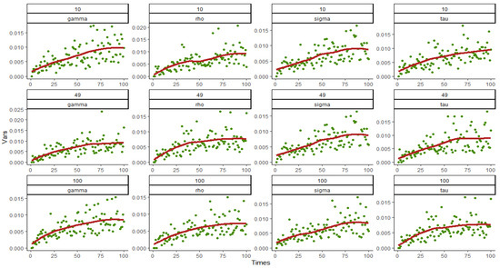
Figure 1.
Variance and fitting curve of when and 100.
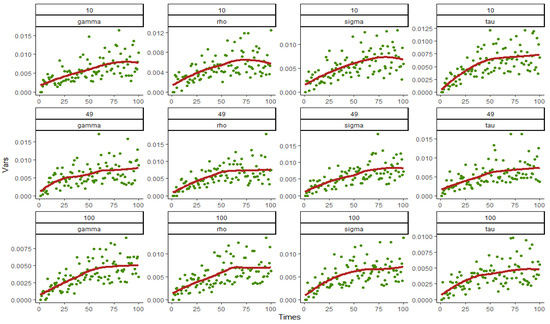
Figure 2.
Variance and fitting curve of when and 100.
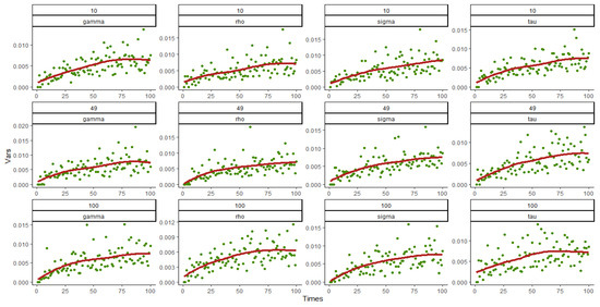
Figure 3.
Variance and fitting curve of when and 100.
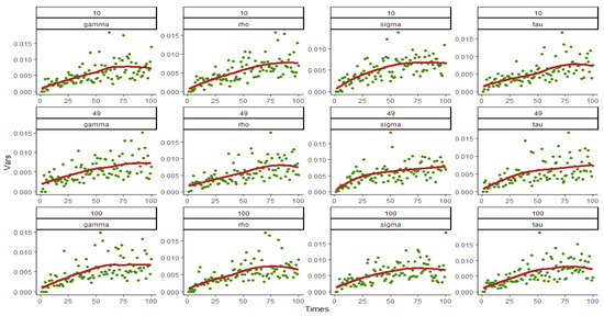
Figure 4.
Variance and fitting curve of when and 100.
Figure 5, Figure 6, Figure 7 and Figure 8 show the graph of the mean value and confidence interval of each parameter in and under various combinations of and , where the blue area is the range covered by the 95% confidence interval, the red broken line is the mean of the parameter estimates, and the yellow line is the true value of the parameters. As can be seen from the figures, due to the small, estimated variances, the means fluctuate very little around the true values, and the ranges of confidence intervals are also relatively stable. In only a few cases, the confidence intervals do not cover the true values, and with the increase in and , the coverage degree becomes higher and higher, that is, the coverage probability (CP) gradually approaches 1.
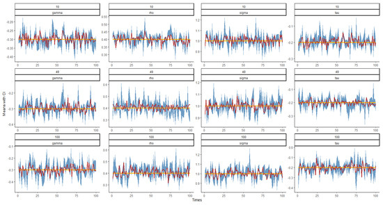
Figure 5.
Plot of the mean and confidence interval of when and 100.
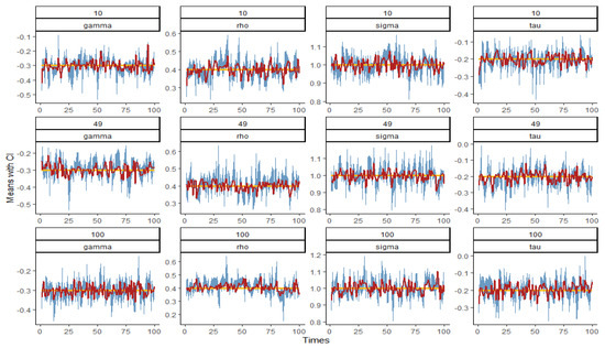
Figure 6.
Plot of the mean and confidence interval of when and 100.
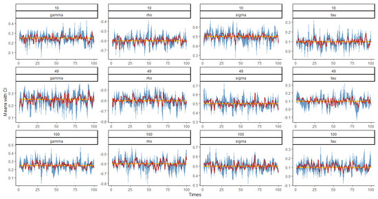
Figure 7.
Plot of the mean and confidence interval of when and 100.
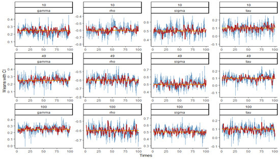
Figure 8.
Plot of the mean and confidence interval of when and 100.
Table 3 shows the average absolute error and variance of the estimates of the unknown function under different samples. By comparing six simulation results under the initial values of different parameters, we can see that under the limited sample, when the period number T is fixed, the deviation between the estimated value and the true value of decreases with the increase in the sample size n, which is mainly represented as the MADE values decrease. This indicates that when T is the same, the estimated values of the parameters will converge with the increase in n; when n is fixed, the deviation between the estimated values and their true value will also decrease with the increase in T. Combining the above two results, it is not difficult to draw the following conclusion: the estimated values will converge to the true values of the parameters with the increase in n and T, which is consistent with the theoretical result of Theorem 3.
Table 3.
Performance of unknown function estimators .
5. Empirical Application: Spatial Spillovers in the Yangtze River Delta
We selected the panel data of 16 cities in the Yangtze River Delta region (Shanghai, Hangzhou, Jiaxing, Huzhou, Ningbo, Shaoxing, Zhoushan, Nanjing, Suzhou, Wuxi, Changzhou, Zhenjiang, Nantong, Yangzhou, Taizhou, and Taizhou) from 2019 to 2021 (data source: Statistical Yearbook of Shanghai, Zhejiang and Jiangsu 2020–2022) to study the relationship between urban tourism development and economic growth in the Yangtze River Delta (YRD). The YRD city cluster is an important intersection area of the “Belt and Road” and the Yangtze River Economic Belt. It plays a pivotal strategic role in China’s modernization and opening-up pattern and is an important platform for China to participate in international competition and an important leader in economic and social development. The YRD city cluster has a vast economic hinterland, modern river and seaports and airports, a relatively sound highway network, leading the country to having an increasing density of road and rail transportation lines, and a three-dimensional comprehensive transportation network, which has important conditions for economic agglomeration. Economic agglomeration is a general state of economic development, representing the geographical and spatial concentration of economic activities. Due to the influence of objective factors such as location condition, ecological environment, development basis, and market development degree, there are significant differences in the tourism development modes of the different cities. However, there are close economic relations between neighboring cities in space, that is, the development of tourism in a certain region not only has a direct impact on the local economy but also has a spillover effect on the economy of its neighboring region. In addition to the spatial lag in the same period, there may also be time and space lag or diffusion, that is, under the premise of spatial interaction between regions, the spatial and temporal linkage of inter-regional tourism development and economic growth will be further enhanced. Therefore, the spatial panel analysis of the spatial spillover effect of economic agglomeration can reveal the possible economic agglomeration phenomenon between regions from the temporal and spatial dimensions, and more objectively and scientifically study the structure and process of regional economic development.
Let denote the gross domestic product (GDP) in city at period . The spatial weights matrix is and if cities and share the same border and otherwise. The tourism dynamic variables are constructed by the number of tourists travelling to every city at period , including international inbound tourists and domestic tourists, which are recorded as and , respectively. GDP is likely to be influenced by a number of macroeconomic factors, which are reflected by fixed effects. The model consists of:
First of all, we fit the data in the ‘nlme’ package of R language to obtain the form of the non-parametric part as follows:
The estimated results of parameters and are shown in Table 4, which all pass the 1% significance test and reveal interesting spatial patterns. Since the expression is in power exponential form, it means that the increase in tourist numbers in a region has a positive impact on local economic development, which is consistent with the inference. The power index () of domestic tourists is negative, and the index () of international inbound tourists is positive, indicating that the increase in international inbound tourist arrivals will greatly promote local economic development, but the increase in domestic tourists will weaken some economic growth generated by tourism. This is related to the consumption habits of domestic tourists and the local tourism reception capacity: first, domestic tourists usually use various preferential and discount apps to book tickets and accommodation in advance, while foreign tourists lack understanding and conditions for this, and second, tourist souvenirs are an important part of tourism profits. They are highly attractive to international tourists, while domestic tourists often choose to buy them online rather than in scenic areas. Finally, China is a populous country, and the local tourism reception capacity is limited. If there are too many domestic tourists at the same time, such as during holidays, it will inevitably affect the travel and consumption experience of foreign tourists. On the other hand, the parameter SDPD model is a linear relationship with a predetermined part of the equation, which is obviously inconsistent with the actual data relationship and may lead to completely different conclusions, which is wrong. In the parametric SDPD model, the linear relationship at is defined in advance, which is obviously inconsistent with the actual data relationship and may lead to completely different and biased conclusions.
Table 4.
Estimation of the non-parametric function.
Table 5 reports the estimated results. Firstly, it shows that the economic development of a city has a positive impact on the neighboring region (), that is, a city with a high degree of economic activity leads to the growth of the economic activity of the neighboring city through knowledge spillover, technological innovation, industrial experience, etc. The spatial agglomeration phenomenon of economic development in the YRD region shows a positive spatial correlation. The positive time lag coefficient () reflects that the economic development of each city in the previous period has a positive impact on itself from 2019 to 2021. This is consistent with the positioning that these 16 cities are the most economically developed and the most valuable urban agglomerations in China. These cities have already determined their own development direction and needs, and with the support of national policies and talents, economic and social development has been steadily improving year on year. Note that and diffusion () have opposite signs, which is a very enlightening discovery. This shows that although the 16 cities are urban clusters that develop together and help each other, their economic development structures are different. Factors that produce spatial effects at the same time, such as industry experience, may be able to learn and emulate in the short term, but they are not suitable for long-term application. Local governments need to develop characteristic economies according to their own economic structure and regional characteristics. On the other hand, the fixed effect () is positive, indicating that the regional economic development process has unique characteristics that do not change with time, including additional individual effects and time effects such as in special cases. There, it is necessary to use the NSDPD model with fixed effect.
Table 5.
Estimation of economic development.
6. Conclusions and Future Work
In this paper, the SDPD model with fixed effects was extended to a non-parametric form, which relaxed the setting that the influence of explanatory variables is a known linear or nonlinear parameter structure, so that the influence of explanatory variables can be any unknown function satisfying certain conditions. Then, we proposed a PML method to estimate the spatial correlation coefficients and unknown functions. The theoretical proof showed that the parameters and non-parametric estimators obtained by the PML method were consistent under certain regular conditions. Numerical simulation showed that the estimator has a good small sample property, and the estimation accuracy increased with the increase in the sample size and time periods.
So far, represents space-specific effects, which controls all variables with fixed space and constant time in the model. It may be of interest to allow more extensive forms of , such as interactive fixed effects in [9], time-varying regression coefficients, time-varying spatial coefficients, time-varying spatial weight matrices, etc., even in the non-fixed space case or completely at random. In terms of theoretical development, our results can be extended to allow for time-varying regression coefficients but may not apply to other types of heterogeneity. Furthermore, the cross-sectional heteroskedasticity (space-varying error variances) in the NSDPD model is another interesting extension to consider. It is a good idea to relax the condition from the assumption of homoscedasticity to the assumption that the random error is sequential and cross-sectional dependent. These models and methods would be much more challenging than the already quite challenging works presented in this paper and will be the topic of our future research.
Author Contributions
Conceptualization, M.Z. and B.T.; methodology, M.Z. and B.T.; software, M.Z.; validation, M.Z. and B.T.; formal analysis, M.Z. and B.T.; investigation, M.Z. and B.T.; resources, M.Z.; data curation, M.Z.; writing—original draft preparation, M.Z.; writing—review and editing, M.Z. and B.T.; visualization, M.Z. and B.T.; supervision, B.T.; project administration, B.T.; funding acquisition, B.T. All authors have read and agreed to the published version of the manuscript.
Funding
This research was funded by [National Natural Science Foundation of China] grant number [91646106].
Data Availability Statement
The data presented in this study are available on request from the corresponding author. The data are not publicly available due to the requirements of related projects supported by [National Natural Science Foundation of China].
Conflicts of Interest
The authors declare no conflict of interest.
Appendix A. Some Basic Lemmas
Proof of Lemma 3.
From , we have . Hence:
where using and ,
Using Lemma 1:
As and are bounded in , we have uniformly in θ in Θ. Using the fact that is bounded away from zero in and ,
uniformly at . □
Proof of Lemma 4.
(similar to Ref. [2]). From and , we have:
where , , and , where:
According to Lemma 1, the third term , and is uniformly in in because it is a polynomial function in θ, and Θ is a bounded set. The second term is equal to , where , which are polynomial functions of , that is, uniformly in θ. Using in the first term, we have:
where
To prove is uniformly equicontinuous for , the following four conditions must be true: (1) is uniformly continuous: is bounded away from zero in , so (1) is obvious. (2) is uniformly equicontinuous: we know , where is between and . Because is UB, uniformly in in , is bounded. Hence, (2) is true. (3) The first term, that is, ’ is uniformly equicontinuous: both and are bounded, with . Hence, (3) is true. (4) is uniformly equicontinuous: by and , we have:
And because and are UB, (4) is true. □
Proof of Lemma 5.
We can follow Lee (2004) by using a contradiction to prove the result. Firstly, we assume where , and are scalars. Next, for , we need to prove that implies . If this is true, then columns of would be linear independent and would be nonsingular.
From (15):
where , , , . Hence, implies:
The first and third equations imply, and , respectively. By eliminating and , the second equation becomes .
Assume under Assumption 9 and is nonsingular, the above formula is true only if , that is . The information matrix is nonsingular. □
Appendix B. Proof of the Theoretical Results
Proof of Theorem 1.
As , at , (10) implies . Then, we have:
Consider the process , for a period t, the log likelihood function of it is:
Let be the expectation operator for , we have:
Through the information inequality, . Thus, for any . Also, is a quadratic function of and . Under the condition that is nonsingular, whenever , so is globally identified. Given is the unique maximizer of . Hence, is globally identified. Combined with uniform convergence and equicontinuity in Lemma 4–5, the consistency follows. □
Proof of Theorem 2.
From proof of Theorem 1, . When is singular, and cannot be identified from . Global identification requires that the limit of is strictly less than zero.TABLE As through the information inequality, is equivalent to:
(See Lee (2004)). After and are identified, given , can be identified from . Combined with the uniform convergence and equicontinuity in Lemma 4–5, the consistency follows. □
Proof of Theorem 3.
As (7), we have ,
From Lemma 6 and Assumption 8:
- if is odd, ,
- if is even, . □
References
- Neyman, J.; Scott, E.L. Consistent estimates based on partially consistent observations. Econometrica 1948, 16, 1–32. [Google Scholar] [CrossRef]
- Yu, J.; de Jong, R.; Lee, L.F. Quasi-maximum likelihood estimators for spatial dynamic panel data with fixed effects when both n and T are large. J. Econom. 2008, 146, 118–134. [Google Scholar] [CrossRef]
- Lee, L.F.; Yu, J. Estimation of spatial panel model with fixed effects. Econometrics 2010, 154, 165–185. [Google Scholar] [CrossRef]
- Lee, L.F.; Yu, J. A spatial dynamic panel data model with both time and individual fixed effects. Econom. Theory 2010, 26, 564–597. [Google Scholar] [CrossRef]
- Yu, J.; de Jong, R.; Lee, L.F. Estimation for spatial dynamic panel data with fixed effects: The case of spatial cointegration. J. Econom. 2012, 167, 16–37. [Google Scholar] [CrossRef]
- Jin, F.; Lee, L.F.; Yu, J. First difference estimation of spatial dynamic panel data models with fixed effects. Econ. Lett. 2020, 189, 109010. [Google Scholar] [CrossRef]
- Lin, X.; Carroll, R.J. Nonparametric function estimation for clustered data when the predictor is measured without/with error. J. Am. Stat. Assoc. 2000, 95, 520–534. [Google Scholar] [CrossRef]
- Henderson, D.J.; Carroll, R.J.; Li, Q. Nonparametric estimation and testing of fixed effects panel data models. J. Econom. 2008, 144, 257–275. [Google Scholar] [CrossRef] [PubMed]
- Shi, W.; Lee, L.F. Spatial dynamic panel data models with interactive fixed effects. Econometrics 2017, 197, 323–347. [Google Scholar] [CrossRef]
Disclaimer/Publisher’s Note: The statements, opinions and data contained in all publications are solely those of the individual author(s) and contributor(s) and not of MDPI and/or the editor(s). MDPI and/or the editor(s) disclaim responsibility for any injury to people or property resulting from any ideas, methods, instructions or products referred to in the content. |
© 2023 by the authors. Licensee MDPI, Basel, Switzerland. This article is an open access article distributed under the terms and conditions of the Creative Commons Attribution (CC BY) license (https://creativecommons.org/licenses/by/4.0/).