Initial Coefficient Bounds for Bi-Univalent Functions Related to Gregory Coefficients

Abstract

In this article we introduce three new subclasses of the class of bi-univalent functions $\Sigma$, namely ${\mathfrak{HG}}_{\Sigma }$, ${\mathfrak{GM}}_{\Sigma }\left(\mu \right)$ and ${\mathfrak{G}}_{\Sigma }\left(\lambda \right)$, by using the subordinations with the functions whose coefficients are Gregory numbers. First, we evidence that these classes are not empty, i.e., they contain other functions besides the identity one. For functions in each of these three bi-univalent function classes, we investigate the estimates $\left|a_2\right|$ and $\left|a_3\right|$ of the Taylor–Maclaurin coefficients and Fekete–Szegő functional problems. The main results are followed by some particular cases, and the novelty of the characterizations and the proofs may lead to further studies of such types of similarly defined subclasses of analytic bi-univalent functions.

1. Definitions and Preliminaries

Let $\mathcal{A}$ denote the class of all analytic (holomorphic) functions f defined in the open unit disk

$$\mathbb{D}:=\{z\in \mathbb{C}:|z|<1\}$$

and normalized by the conditions $f\left(0\right)=0$ and $f^{\prime }\left(0\right)=1$. Thus, each $f\in \mathcal{A}$ has a Taylor–Maclaurin series expansion of the form

$$f\left(z\right)=z+\sum _{n=2}^{\infty }{a}_n{z}^n,z\in \mathbb{D}.$$

(1)

Further, let $\mathcal{S}$ denote the class of all functions $f\in \mathcal{A}$ that are univalent in $\mathbb{D}$. If $F_1,F_2\in \mathcal{H},$ we say that $F_1$ is subordinate to $F_2$, written as $F_1\prec F_2$ or $F_1\left(z\right)\prec F_2\left(z\right)$ if there exists $\varpi \in \Omega$, such that $F_1\left(z\right)=F_2\left(\varpi \left(z\right)\right)$, $z\in \mathbb{D}$. Moreover, if $F_2$ is univalent in $\mathbb{D}$, then, equivalently, we have

$$F_1\left(z\right)\prec F_2\left(z\right)\iff F_1\left(0\right)=F_2\left(0\right)\mathrm{and}{F}_1\left(\mathbb{D}\right)\subset F_2\left(\mathbb{D}\right).$$

(2)

The Koebe one-quarter theorem confirms that the image of $\mathbb{D}$ under every univalent function $f\in \mathcal{A}$ comprises a disk of radius $\frac{1}{4}$. Thus, every function $f\in \mathcal{S}$ has an inverse $f^{-1}$, defined by

$$f^{-1}\left(f\left(z\right)\right)=z,z\in \mathbb{D},$$

and

$$f\left(f^{-1}\left(w\right)\right)=w,\left|w\right|<r_0\left(f\right),r_0\left(f\right)\ge \frac{1}{4}.$$

Suppose that $f^{-1}$ has an analytic continuation to $\mathbb{D}$. Then, the function f is said to be bi-univalent in $\mathbb{D}$ if both f and $f^{-1}$ are univalent in $\mathbb{D}$ and are represented by

$$g\left(w\right):=f^{-1}\left(w\right)=w-a_2{w}^2+\left(2a_2^2-a_3\right)w^3-\left(5a_2^3-5a_2{a}_3+a_4\right)w^4+\dots$$

(3)

Let $\Sigma$ denote the class of bi-univalent functions defined in $\mathbb{D}.$ The functions

$$\frac{z}{1-z},log\frac{1}{1-z},log\sqrt{\frac{1+z}{1-z}.}$$

are in $\Sigma$. However, the familiar Koebe function is not a member of $\Sigma$, while other common examples of analytic functions in $\mathbb{D}$, such as

$$\frac{2z-z^2}{2}\mathrm{and}\frac{z}{1-z^2},$$

are also not members of $\Sigma$. Lewin [1] examined the class $\Sigma$ and found it to be $a_2<1.51$. Subsequently, Brannan and Clunie [2] conjectured that $a_2<\sqrt{2}$. On the other hand, Netanyahu [3] showed that $\underset{f\in \Sigma }{max}{a}_2=4/3$. The problem of estimating the coefficient for each Taylor–Maclaurin coefficient $a_n$ of $n\in \mathbb{N}$, $n\ge 3$, is still considered an open problem.

Analogous to the familiar subclasses ${\mathcal{S}}^{*}\left(\rho \right)$ and $\mathcal{K}\left(\rho \right)$ of starlike and convex function of order $\rho$, $0\le \rho <1$, respectively, Brannan and Taha [4] (see also [5]) introduced certain subclasses of $\Sigma$, namely the subclasses ${\mathcal{S}}_{\Sigma }^{*}\left(\rho \right)$ and ${\mathcal{K}}_{\Sigma }\left(\rho \right)$ of bi-starlike functions and of bi-convex functions of order $\rho$, $0\le \rho <1$, respectively. For $f\in {\mathcal{S}}_{\Sigma }^{*}\left(\rho \right)$ and $f\in {\mathcal{K}}_{\Sigma }\left(\rho \right)$, they found non-sharp estimates $|a_2|$ and $|a_3|$ of initial Taylor–Maclaurin coefficients. In fact, Srivastava et al. [6] considered the study of analytic and bi-univalent functions in recent years for some intriguing examples of functions and characterization of the class $\Sigma$ (see [6,7,8,9,10,11,12,13,14]).

Fekete–Szegő functional $|a_3-\mu a_2^2|$ of $f\in \mathcal{S}$ is well known due to its rich history of application in geometric function theory. Its origin is in the disproof of the hypothesis of Fekete and Szegő [15] by Littlewood and Paley, finding that the coefficients of odd univalent functions are bounded by unity. Since then, this work has received great attention, especially for many subclasses of $\mathcal{S}$. The problem of finding the sharp boundary of the $f\in \mathcal{S}$ for any complex $\mu$ is often referred to as the classical Fekete–Szegő problem (or inconsistencies).

Gregory coefficients ${\mathrm{\Lambda }}_n$. Gregory coefficients, also known as reciprocal logarithmic numbers, Bernoulli numbers of the second kind, or Cauchy numbers of the first kind, are the decreased rational numbers ${\displaystyle \frac{1}{2}},-{\displaystyle \frac{1}{12}},{\displaystyle \frac{1}{24}},-{\displaystyle \frac{19}{720}},\dots$. They occur in the Maclaurin series expansion of the reciprocal logarithm

$$\frac{z}{log(1+z)}=1+\frac{1}{2}z-\frac{1}{12}{z}^2+\frac{1}{24}{z}^3-\frac{19}{720}{z}^4+\dots ,z\in \mathbb{D}.$$

These numbers are named after James Gregory, who introduced them in 1670 in the numerical integration context. They were later revived by many mathematicians and frequently appear in the works of modern authors, such as Laplace, Mascheroni, Fontana, Bessel, Clausen, Hermit, Pearson, and Fisher.

In this paper, we consider the generating function of the Gregory coefficients ${\mathrm{\Lambda }}_n$ (see [16,17]) to be given by

$$\begin{array}{cc}\hfill \mathfrak{G}\left(z\right)& =\frac{z}{log(1+z)}=\sum _{n=0}^{\infty }{\mathrm{\Lambda }}_n{z}^n\hfill \\ \hfill & =1+\frac{1}{2}z-\frac{1}{12}{z}^2+\frac{1}{24}{z}^3-\frac{19}{720}{z}^4+\frac{3}{160}{z}^5-\frac{863}{\mathrm{60,480}}{z}^6+\dots ,\hfill \end{array}$$

where $z\in \mathbb{D}$ and the function log is considered at the main branch, i.e., $log1=0$. Clearly, ${\mathrm{\Lambda }}_n$ for some values of $n\in \mathbb{N}$ are

$${\mathrm{\Lambda }}_0=1,{\mathrm{\Lambda }}_1=\frac{1}{2},{\mathrm{\Lambda }}_2=-\frac{1}{12};{\mathrm{\Lambda }}_3=\frac{1}{24},{\mathrm{\Lambda }}_4=-\frac{19}{720},{\mathrm{\Lambda }}_5=\frac{3}{160},\mathrm{and}{\mathrm{\Lambda }}_6=-\frac{863}{\mathrm{60,480}}.$$

To find the upper bound for the Taylor coefficients has been one of the critical topics of research in geometric characteristics, because it offers numerous properties for many subclasses of $\mathcal{A}$. Therefore, we are interested in the subsequent problem in this section: find $sup |a_n|$ if $n=2,3,\dots$ for subclasses of $\mathcal{S}$. In particular, the bound for $a_2$ offers growth and distortion theorems for features of these subclasses. Further, the use of the Hankel determinant is relevant (which also deals with the bounds of the coefficients), and we also mention that Cantor [18] proved that “if the ratio of two bounded analytic features in $\mathbb{D}$, then the function is rational”. In this article, for the first time, we make an attempt to improve the initial non-sharp coefficients for certain subclasses of $\Sigma$.

2. Coefficient Bounds of the Class ${\mathfrak{HG}}_{\mathit{\Sigma }}$

In 2010, Srivastava et al. [6] revived the study of analytic and bi-univalent functions. Inspired by this, in this section, we consider the class of analytic bi-univalent functions related to the generating functions of the Gregory coefficients to obtain initial coefficients $|a_2|$ and $|a_3|$.

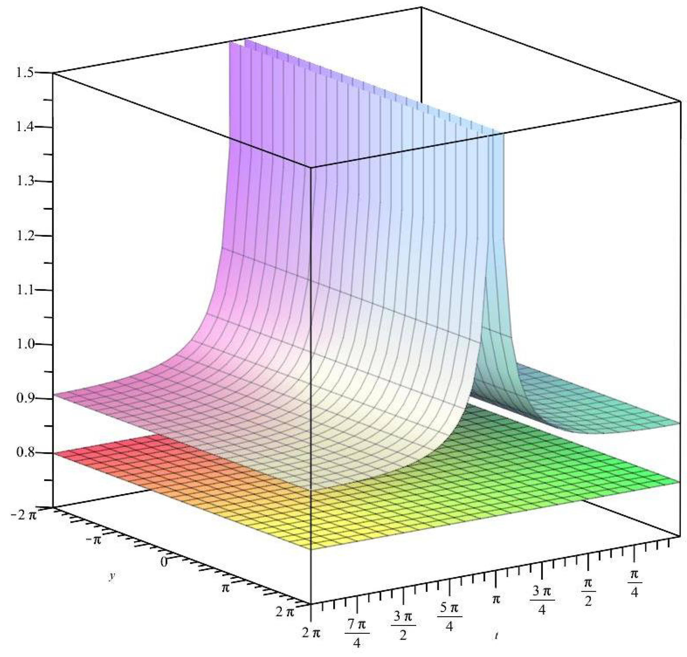
Definition 1.

A function $f\in \Sigma$ given by (1) is said to be in the class ${\mathfrak{HG}}_{\Sigma }$ if the following subordinations

$$\begin{array}{ccc}& & f^{\prime }\left(z\right)\prec \mathfrak{G}\left(z\right),\hfill \end{array}$$

(4)

$$\begin{array}{ccc}& & g^{\prime }\left(w\right)\prec \mathfrak{G}\left(w\right)\hfill \end{array}$$

(5)

are satisfied, and the function $g\left(w\right)=f^{-1}\left(w\right)$ is defined by (3).

Remark 1.

1. For the function $\mathfrak{G}$, we have $\mathfrak{G}\left(0\right)=1$, ${\mathfrak{G}}^{\prime }\left(0\right)\ne 0$, and using the 3D plot of the MAPLE™ computer software, we obtain that the image of the open unit disk $\mathbb{D}$ by the function

$$\mathrm{U}\left(z\right):=Re\frac{z{\mathfrak{G}}^{\prime }\left(z\right)}{\mathfrak{G}\left(z\right)-1},z\in \mathbb{D},$$

is positive; hence, $\mathfrak{G}$ is a starlike (and also univalent) function with respect to the point 1 (see Figure 1).

2. We would like to emphasize that the class ${\mathfrak{HG}}_{\Sigma }$ is not empty. Thus, if we consider $f_{*}\left(z\right)={\displaystyle \frac{z}{1-az}}$, $\left|a\right|\le 1$, then it is easy to check that $f_{*}\in \mathcal{S}$, and, moreover, $f_{*}\in \Sigma$ with $g_{*}\left(w\right)=f_{*}^{-1}\left(w\right)={\displaystyle \frac{w}{1+aw}}$.

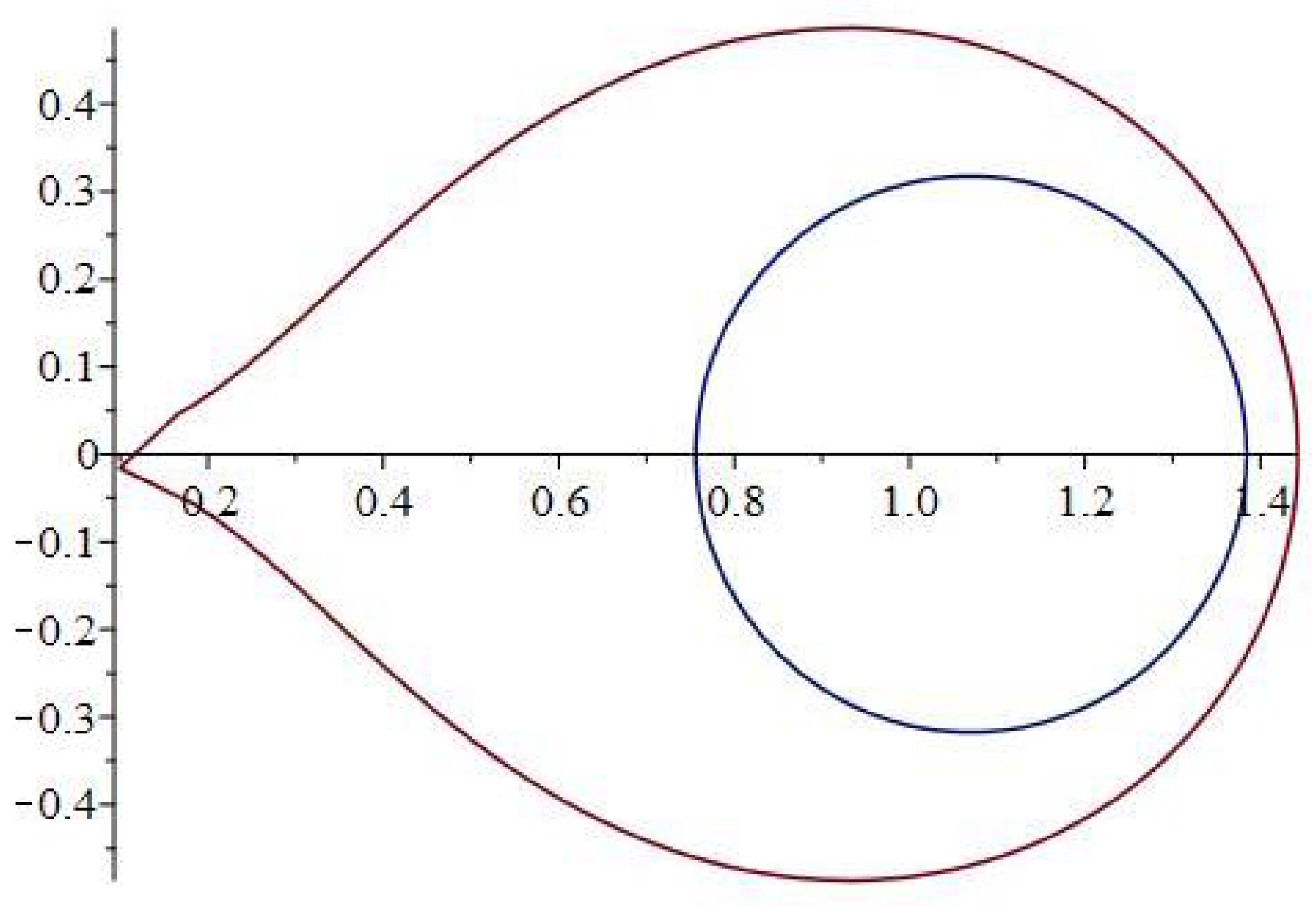
Using the fact that $f_{*}^{\prime }(-az)=g_{*}^{\prime }\left(az\right)$ for all $z\in \mathbb{D}$, it follows that $f_{*}^{\prime }\left(\mathbb{D}\right)=g_{*}^{\prime }\left(\mathbb{D}\right)$. For the particular case $a=0.15$, using the 2D plot of the MAPLE™ computer software, we obtain the image of the boundary $\partial \mathbb{D}$ by the functions $f_{*}^{\prime }$, $g_{*}^{\prime }$, and $\mathfrak{G}$, shown in Figure 2. Since $\mathfrak{G}$ is univalent in $\mathbb{D}$, the previous explanation yields that the subordinations $f_{*}^{\prime }\left(z\right)\prec \mathfrak{G}\left(z\right)$ and $g_{*}^{\prime }\left(w\right)\prec \mathfrak{G}\left(w\right)$ hold whenever $f_{*}^{\prime }\left(0\right)=g_{*}^{\prime }\left(0\right)=\mathfrak{G}\left(0\right)$ and $f_{*}^{\prime }\left(\mathbb{D}\right)=g_{*}^{\prime }\left(\mathbb{D}\right)\subset \mathfrak{G}\left(\mathbb{D}\right)$ (see Figure 2). In conclusion, $f_{*}\in {\mathfrak{HG}}_{\Sigma }$; hence, the class ${\mathfrak{HG}}_{\Sigma }$ is not empty and contains other functions besides the identity.

In our first results, we obtain better upper bounds for $|a_2|$ and $|a_3|$ for $f\in {\mathfrak{HG}}_{\Sigma }$ given in Definition 1. Further, we use the following lemmas, which were introduced by Zaprawa in [19,20], and we discuss the Fekete–Szegő functional problems [15].

Let $\mathcal{P}\left(\beta \right)$, with $0\le \beta <1$, denote the class of analytic functions p in $\mathbb{D}$ with $p\left(0\right)=1$ and $Rep\left(z\right)>\beta$, $z\in \mathbb{D}$. In particular, we use the notation $\mathcal{P}$ instead of $\mathcal{P}\left(0\right)$ for the usual Carathéodory class of functions.

The next two lemmas are used in our study.

Lemma 1

([21]). If $p\in \mathcal{P}$ has the form $p\left(z\right)=1+c_{1}z+c_2{z}^2+\dots$, $z\in \mathbb{D}$, then

$$|c_n| \le 2,n\ge 1,$$

(6)

and this inequality is sharp for each $n\in \mathbb{N}$.

We mention that this inequality is the well-known result of the Carathéodory lemma [21] (see also [22], Corollary 2.3, p. 41, [23], Carathéodory’s Lemma, p. 41).

The second lemma is a generalization of Lemma 6 from [20], which can be obtained for $l=1$.

Lemma 2

([20], Lemma 7, p. 2). Let $k,l\in \mathbb{R}$ and $z_1,z_2\in \mathbb{C}$. If $|z_1| <R$ and $|z_2| <R$; then,

$$|(k+l)z_1+(k-l)z_2| \le \left\{\begin{array}{ccc}2\left|k\right|R,\hfill & for\hfill & \left|k\right|\ge \left|l\right|,\hfill \\ 2\left|l\right|R,\hfill & for\hfill & \left|k\right|\le \left|l\right|.\hfill \end{array}\right.$$

The following result gives the upper bounds for the first two coefficients of the functions that belong to ${\mathfrak{HG}}_{\Sigma }$.

Theorem 1.

If $f\in {\mathfrak{HG}}_{\Sigma }$ is given by (1), then

$$\left|a_2\right|\le \sqrt{\frac{3}{74}}\simeq 0.0234\dots ,and\left|a_3\right|\le \frac{23}{111}\simeq 0.2072\dots$$

Proof. 

If $f\in {\mathfrak{HG}}_{\Sigma }$, from Definition 1, the subordinations (4) and (5) hold. Then, there exists an analytic function u in $\mathbb{D}$ with $u\left(0\right)=0$ and $\left|u\right(z\left)\right|<1$, $z\in \mathbb{D}$, such that

$$f^{\prime }\left(z\right)=\mathfrak{G}\left(u\left(z\right)\right),z\in \mathbb{D},$$

(7)

and an analytic function v in $\mathbb{D}$ with $v\left(0\right)=0$ and $\left|v\right(w\left)\right|<1$, $w\in \mathbb{D}$, such that

$$g^{\prime }\left(w\right)=\mathfrak{G}\left(v\left(w\right)\right),w\in \mathbb{D}.$$

(8)

Therefore, the function

$$h\left(z\right)=\frac{1+u\left(z\right)}{1-u\left(z\right)}=1+c_{1}z+c_2{z}^2+\dots ,z\in \mathbb{D},$$

belongs to the class $\mathcal{P}$; hence,

$$u\left(z\right)=\frac{c_1}{2}z+\left(c_2-\frac{c_1^2}{2}\right)\frac{z^2}{2}+\left(c_3-c_1{c}_2+\frac{c_1^3}{4}\right)\frac{z^3}{2}+\dots ,z\in \mathbb{D},$$

and

$$\begin{array}{c}\mathfrak{G}\left(u\left(z\right)\right)=1+\frac{c_1}{4}z+\frac{1}{48}\left(-7c_1^2+12c_2\right)z^2+\frac{1}{192}\left(17c_1^3-56c_1{c}_2+48c_3\right)z^3+\dots ,\hfill \\ \hfill z\in \mathbb{D}.\end{array}$$

(9)

The function

$$k\left(w\right)=\frac{1+v\left(w\right)}{1-v\left(w\right)}=1+d_{1}w+d_2{w}^2+\dots ,w\in \mathbb{D},$$

belongs to the class $\mathcal{P}$; therefore,

$$v\left(w\right)=\frac{d_1}{2}w+\left(d_2-\frac{d_1^2}{2}\right)\frac{w^2}{2}+\left(d_3-d_1{d}_2+\frac{d_1^3}{4}\right)\frac{w^3}{2}+\dots ,w\in \mathbb{D},$$

and

$$\begin{array}{c}\mathfrak{G}\left(v\left(w\right)\right)=1+\frac{d_1}{4}w+\frac{1}{48}\left(-7d_1^2+12d_2\right)w^2+\frac{1}{192}\left(17d_1^3-56d_1{d}_2+48d_3\right)w^3+\dots ,\hfill \\ \hfill w\in \mathbb{D}.\end{array}$$

(10)

From the equalities (7) and (8), we obtain that

$$f^{\prime }\left(z\right)=1+\frac{c_1}{4}z+\frac{1}{48}\left(-7c_1^2+12c_2\right)z^2+\dots ,z\in \mathbb{D},$$

(11)

and

$$g^{\prime }\left(w\right)=1+\frac{d_1}{4}w+\frac{1}{48}\left(-7d_1^2+12d_2\right)w^2+\dots ,w\in \mathbb{D}.$$

(12)

Comparing the corresponding coefficients in (11) and (12), we obtain

$$\begin{array}{ccc}& & 2a_2=\frac{c_1}{4},\hfill \end{array}$$

(13)

$$\begin{array}{ccc}& & 3a_3=\frac{c_2}{4}-\frac{7}{48}{c}_1^2,\hfill \end{array}$$

(14)

$$\begin{array}{ccc}& & -2a_2=\frac{d_1}{4},\hfill \end{array}$$

(15)

$$\begin{array}{ccc}& & 3\left(2a_2^2-a_3\right)=\frac{d_2}{4}-\frac{7}{48}{d}_1^2.\hfill \end{array}$$

(16)

From (13) and (15), it follows that

$$c_1=-d_1$$

(17)

and

$$c_1^2+d_1^2=128a_2^2.$$

(18)

If we add the equalities (14) and (16), we obtain

$$6a_2^2=\frac{1}{4}\left(c_2+d_2\right)-\frac{7}{48}\left(c_1^2+d_1^2\right),$$

(19)

and removing the value of $\left(c_1^2+d_1^2\right)$ from (18) in (19), we deduce that

$$a_2^2=\frac{3(c_2+d_2)}{296}.$$

(20)

Using (6) together with the triangle inequality in the relations (13) and (20), it follows that

$$\left|a_2\right|\le \frac{1}{4}=0.25\mathrm{and}\left|a_2\right|\le \sqrt{\frac{3}{74}}\simeq 0.0234\dots$$

which proves our first result.

Moreover, if we subtract (16) from (14), we obtain

$$6\left(a_3-a_2^2\right)=\frac{1}{4}(c_2-d_2)-\frac{7}{48}\left(c_1^2-d_1^2\right),$$

(21)

and in view of (17), the equality (21) becomes

$$a_3=a_2^2+\frac{1}{24}\left(c_2-d_2\right).$$

(22)

The above relation combined with (13) leads to

$$a_3=\frac{c_1^2}{64}+\frac{1}{24}\left(c_2-d_2\right).$$

(23)

Using the triangle inequality and (6), from (23), we obtain

$$\left|a_3\right|\le \frac{1}{16}+\frac{1}{6}=\frac{11}{48}\simeq 0.2291\dots$$

and using our first assertion together with (22), it follows that

$$\left|a_3\right|\le \frac{3}{74}+\frac{1}{6}=\frac{23}{111}\simeq 0.2072\dots ,$$

which completes the proof of our theorem. □

Using the above values for $a_2^2$ and $a_3$, we prove the following Fekete–Szegő-type inequality for the functions of the class ${\mathfrak{HG}}_{\Sigma }$.

Theorem 2.

If $f\in {\mathfrak{HG}}_{\Sigma }$ is given by (1), then, for any $\mu \in \mathbb{R}$, the following inequality holds:

$$\left|a_3-\mu a_2^2\right|\le \left\{\begin{array}{ccc}{\displaystyle \frac{1}{6}},\hfill & \mathit{for}\hfill & \mu \in \left[-{\displaystyle \frac{28}{9}},{\displaystyle \frac{46}{9}}\right],\hfill \\ {\displaystyle \frac{3|1-\mu |}{74}},\hfill & \mathit{for}\hfill & \mu \in \left(-\infty ,-{\displaystyle \frac{28}{9}}\right]\cup \left[{\displaystyle \frac{46}{9}},+\infty \right).\hfill \end{array}\right.$$

Proof. 

If $f\in {\mathfrak{HG}}_{\Sigma }$ has the form (1), from (20) and (22), we obtain

$$a_3-\mu a_2^2=\left(1-\mu \right)\frac{3(c_2+d_2)}{296}+\frac{1}{24}\left(c_2-d_2\right)=\left(h\left(\mu \right)+\frac{1}{24}\right)c_2+\left(h\left(\mu \right)-\frac{1}{24}\right)d_2,$$

where

$$h\left(\mu \right)=\frac{3(1-\mu )}{296}.$$

From Lemma 1 we have $\left|c_2\right|\le 2$ and also $\left|d_2\right|\le 2$. Then, in view of Lemma 2, we obtain

$$\left|a_3-\mu a_2^2\right|\le \left\{\begin{array}{ccc}{\displaystyle \frac{1}{6}},\hfill & \mathrm{for}\hfill & \left|h\left(\mu \right)\right|\le {\displaystyle \frac{1}{24}},\hfill \\ 4\left|h\right(\mu \left)\right|,\hfill & \mathrm{for}\hfill & \left|h\left(\mu \right)\right|\ge {\displaystyle \frac{1}{24}},\hfill \end{array}\right.$$

which is equivalent to our result. □

3. Coefficient Bounds for the Class ${\mathfrak{GM}}_{\mathbf{\Sigma }}\mathbf{\left(}\mathit{\mu }\mathbf{\right)}$

In the second set of results, we obtain the upper bounds for the modules of the first two coefficients for the functions that belong to the class ${\mathfrak{GM}}_{\Sigma }\left(\mu \right)$ defined below; then, we study the Fekete–Szegő functional problems for this function class.

Definition 2.

A function $f\in \Sigma$ given by (1) is said to be in the class ${\mathfrak{GM}}_{\Sigma }\left(\mu \right)$ if the following subordinations hold:

$$\begin{array}{ccc}& & \Phi \left(z\right):=\left(1-\mu \right)\frac{z{f}^{\prime }\left(z\right)}{f\left(z\right)}+\mu \left(1+\frac{z{f}^{″}\left(z\right)}{f^{\prime }\left(z\right)}\right)\prec \mathfrak{G}\left(z\right),\hfill \end{array}$$

(24)

$$\begin{array}{ccc}& & \Psi \left(w\right):=\left(1-\mu \right)\frac{w{g}^{\prime }\left(w\right)}{g\left(w\right)}+\mu \left(1+\frac{w{g}^{″}\left(w\right)}{g^{\prime }\left(w\right)}\right)\prec \mathfrak{G}\left(w\right),\hfill \end{array}$$

(25)

where $0\le \mu \le 1$ and $g\left(w\right)=f^{-1}\left(w\right)$ is as in (3).

By fixing $\mu =0$ or $\mu =1$, we have the following special subclasses.

Remark 2.

1. For $\mu =0$, let ${\mathfrak{GS}}_{\Sigma }:={\mathfrak{GM}}_{\Sigma }\left(0\right)$ be the subclass of functions $f\in \Sigma$ satisfying

$$\frac{z{f}^{\prime }\left(z\right)}{f\left(z\right)}\prec \mathfrak{G}\left(z\right)and\frac{w{g}^{\prime }\left(w\right)}{g\left(w\right)}\prec \mathfrak{G}\left(w\right),$$

with $g\left(w\right)=f^{-1}\left(w\right)$.

Fixing $\mu =1$, let ${\mathfrak{GV}}_{\Sigma }:={\mathfrak{GM}}_{\Sigma }\left(1\right)$ be the subclass of functions $f\in \Sigma$ that satisfy

$$1+\frac{z{f}^{″}\left(z\right)}{f^{\prime }\left(z\right)}\prec \mathfrak{G}\left(z\right)and1+\frac{w{g}^{″}\left(w\right)}{g^{\prime }\left(w\right)}\prec \mathfrak{G}\left(w\right),$$

where $g\left(w\right)=f^{-1}\left(w\right)$.

Remark 3.

We prove that the appropriate choice of the parameter μ in the class ${\mathfrak{GM}}_{\Sigma }\left(\mu \right)$ is not empty. Letting $f_{*}\left(z\right)={\displaystyle \frac{z}{1-az}}$, $\left|a\right|\le 1$, it easily follows that $f_{*}\in \mathcal{S}$, and, additionally, $f_{*}\in \Sigma$ with $g_{*}\left(w\right)=f_{*}^{-1}\left(w\right)={\displaystyle \frac{w}{1+aw}}$.

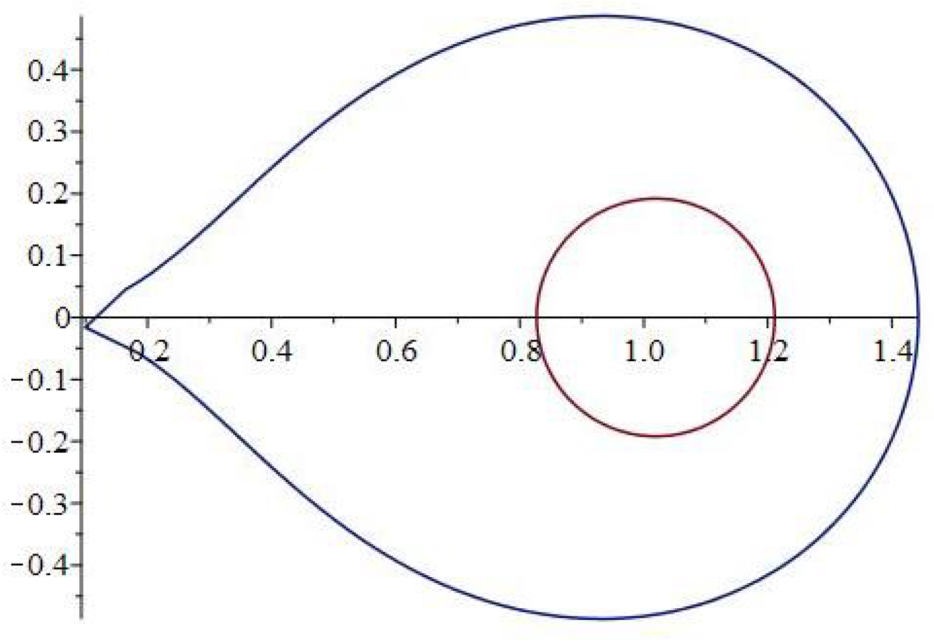
With the notations of (24) and (25), simple computation shows that $\Phi (-az)=\Psi \left(az\right)$ for all $z\in \mathbb{D}$, which implies that $\Phi \left(\mathbb{D}\right)=\Psi \left(\mathbb{D}\right)$. Taking the particular case $a=0.15$ and $\mu =0.9$, using the 2D plot of the MAPLE™ computer software, we obtain the image of the boundary $\partial \mathbb{D}$ by the functions Φ, Ψ, and $\mathfrak{G}$, presented in Figure 3. Using the fact that $\mathfrak{G}$ is univalent in $\mathbb{D}$, the above explanation means that the subordinations $\Phi \left(z\right)\prec \mathfrak{G}\left(z\right)$ and $\Psi \left(w\right)\prec \mathfrak{G}\left(w\right)$ hold whenever $\Phi \left(0\right)=\Psi \left(0\right)=\mathfrak{G}\left(0\right)$ and $\Phi \left(\mathbb{D}\right)=\Psi \left(\mathbb{D}\right)\subset \mathfrak{G}\left(\mathbb{D}\right)$ (see Figure 3). Therefore, $f_{*}\in {\mathfrak{GM}}_{\Sigma }\left(0.9\right)$; hence, the class ${\mathfrak{GM}}_{\Sigma }\left(\mu \right)$ is not empty and contains other functions besides the identity.

Theorem 3.

If $f\in {\mathfrak{GM}}_{\Sigma }\left(\mu \right)$ is given by (1), then

$$|a_2| \le \sqrt{\frac{3}{2(1+\mu )(10+7\mu )}}and\left|a_3\right|\le \frac{7{\mu }^2+29\mu +16}{4(1+\mu )(10+7\mu )(1+2\mu )}.$$

Proof. 

If $f\in {\mathfrak{GM}}_{\Sigma }\left(\mu \right)$ has the form (1), from Definition 2, for some analytic functions in $\mathbb{D}$, namely u and v such that $u\left(0\right)=v\left(0\right)=0$ and $\left|u\right(z\left)\right|<1$, $\left|v\right(w\left)\right|<1$ for all $z,w\in \mathbb{D}$, we can write

$$\left(1-\mu \right)\frac{z{f}^{\prime }\left(z\right)}{f\left(z\right)}+\mu \left(1+\frac{z{f}^{″}\left(z\right)}{f^{\prime }\left(z\right)}\right)=\mathfrak{G}\left(u\left(z\right)\right),z\in \mathbb{D},$$

(26)

and

$$\left(1-\mu \right)\frac{w{g}^{\prime }\left(w\right)}{g\left(w\right)}+\mu \left(1+\frac{w{g}^{″}\left(w\right)}{g^{\prime }\left(w\right)}\right)=\mathfrak{G}\left(v\left(w\right)\right),w\in \mathbb{D}.$$

(27)

From the equalities (26) and (27), combined with (9) and (10), we obtain

$$\left(1-\mu \right)\frac{z{f}^{\prime }\left(z\right)}{f\left(z\right)}+\mu \left(1+\frac{z{f}^{\prime \prime }\left(z\right)}{f^{\prime }\left(z\right)}\right)=1+\frac{c_1}{4}z+\frac{1}{48}\left(-7c_1^2+12c_2\right)z^2+\dots ,z\in \mathbb{D},$$

(28)

and

$$\left(1-\mu \right)\frac{w{g}^{\prime }\left(w\right)}{g\left(w\right)}+\mu \left(1+\frac{w{g}^{\prime \prime }\left(w\right)}{g^{\prime }\left(w\right)}\right)=1+\frac{d_1}{4}w+\frac{1}{48}\left(-7d_1^2+12d_2\right)w^2+\dots ,w\in \mathbb{D}.$$

(29)

Equating the first coefficients of (28) and (29), we have

$$\begin{array}{ccc}& & \left(1+\mu \right)a_2=\frac{c_1}{4},\hfill \end{array}$$

(30)

$$\begin{array}{ccc}& & 2\left(1+2\mu \right)a_3-\left(1+3\mu \right)a_2^2=\frac{1}{48}\left(-7c_1^2+12c_2\right),\hfill \end{array}$$

(31)

$$\begin{array}{ccc}& & -\left(1+\mu \right)a_2=\frac{d_1}{4},\hfill \end{array}$$

(32)

$$\begin{array}{ccc}& & \left(3+5\mu \right)a_2^2-2\left(1+2\mu \right)a_3=\frac{1}{48}\left(-7d_1^2+12d_2\right).\hfill \end{array}$$

(33)

From (30) and (32), it follows that

$$c_1=-d_1$$

(34)

and

$$2{\left(1+\mu \right)}^2{a}_2^2=\frac{c_1^2+d_1^2}{16},$$

(35)

i.e.,

$$a_2^2=\frac{c_1^2+d_1^2}{32{\left(1+\mu \right)}^2}.$$

(36)

If we add (31) and (33), we obtain

$$2\left(1+\mu \right)a_2^2=\frac{1}{4}\left(c_2+d_2\right)-\frac{7}{48}\left(c_1^2+d_1^2\right),$$

(37)

and by substituting (35) for $\left(c_1^2+d_1^2\right),$ in (37), we obtain

$$\frac{2}{3}\left[3\left(1+\mu \right)+7{(1+\mu )}^2\right]a_2^2=\frac{c_2+d_2}{4},$$

i.e.,

$$a_2^2=\frac{3(c_2+d_2)}{8\left[3(1+\mu )+7{(1+\mu )}^2\right]}=\frac{3(c_2+d_2)}{8(1+\mu )(10+7\mu )}.$$

(38)

For the same reasons as in the proof of Theorem 1, using (6) in (30), (36), and (38), we find that

$$\left|a_2\right|\le \frac{1}{2(1+\mu )}=:A\left(\mu \right)\mathrm{and}\left|a_2\right|\le \sqrt{\frac{3}{2(1+\mu )(10+7\mu )}}=:B\left(\mu \right).$$

Simple computations shows that $A\left(\mu \right)>B\left(\mu \right)$ whenever $0\le \mu \le 1$; hence, we obtain our first inequality.

Moreover, if we subtract (31) from (33), we obtain

$$4\left(1+2\mu \right)\left(a_3-a_2^2\right)=\frac{c_2-d_2}{4}-\frac{7}{48}\left(c_1^2-d_1^2\right).$$

(39)

Using (34) and (36), the relation (39) becomes

$$a_3=\frac{c_1^2+d_1^2}{32{\left(1+\mu \right)}^2}+\frac{c_2-d_2}{16\left(1+2\mu \right)},$$

(40)

and using the triangle inequality together with (6), we conclude that

$$\left|a_3\right|\le \frac{1}{4{\left(1+\mu \right)}^2}+\frac{1}{4\left(1+2\mu \right)}=\frac{{\mu }^2+4\mu +2}{4{(1+\mu )}^2(1+2\mu )}=:C\left(\mu \right).$$

Moreover, taking into the account the relation (36), Formula (40) could be rewritten as

$$a_3=a_2^2+\frac{c_2-d_2}{16\left(1+2\mu \right)},$$

(41)

and from the triangle inequality together with (6), using the fact that $|a_2|\le B\left(\mu \right)$, it follows that

$$\left|a_3\right|\le \frac{3}{2(1+\mu )(10+7\mu )}+\frac{1}{4\left(1+2\mu \right)}=\frac{7{\mu }^2+29\mu +16}{4(1+\mu )(10+7\mu )(1+2\mu )}=:D\left(\mu \right).$$

Since it is easy to check that $C\left(\mu \right)>D\left(\mu \right)$ for $0\le \mu \le 1$, our second inequality is proven. □

The next result gives an upper bound for the Fekete–Szegő functional for the class ${\mathfrak{GM}}_{\Sigma }\left(\mu \right)$.

Theorem 4.

If $f\in {\mathfrak{GM}}_{\Sigma }\left(\mu \right)$ is given by (1), then

$$\left|a_3-k{a}_2^2\right|\le \left\{\begin{array}{ccc}{\displaystyle \frac{1}{4(1+2\mu )}},\hfill & for\hfill & \left|{\rm Y}\left(k\right)\right|\le {\displaystyle \frac{1}{16\left(1+2\mu \right)}},\hfill \\ 4\left|{\rm Y}\left(k\right)\right|,\hfill & for\hfill & \left|{\rm Y}\left(k\right)\right|\ge {\displaystyle \frac{1}{16\left(1+2\mu \right)}},\hfill \end{array}\right.$$

(42)

where

$${\rm Y}\left(k\right)=\frac{3(1-k)}{8(1+\mu )(10+7\mu )}.$$

(43)

Proof. 

If $f\in {\mathfrak{GM}}_{\Sigma }\left(\mu \right)$, using the same notations as in the proof of the previous theorem, from (38) and (41), we obtain

$$\begin{array}{cc}\hfill a_3-k{a}_2^2& =\left(1-k\right)\frac{3(c_2+d_2)}{8(1+\mu )(10+7\mu )}+\frac{c_2-d_2}{16\left(1+2\mu \right)}\hfill \\ \hfill & =\left[{\rm Y}\left(k\right)+\frac{1}{16\left(1+2\mu \right)}\right]c_2+\left[{\rm Y}\left(k\right)-\frac{1}{16\left(1+2\mu \right)}\right]d_2,\hfill \end{array}$$

where ${\rm Y}\left(k\right)$ is given by (43). According to Lemma 2, from the inequality (6), we obtain the conclusion (42). □

For $\mu =0$ and $\mu =1$, the above theorem reduces to the following two results, respectively.

Example 1.

1. If $f\in {\mathfrak{GS}}_{\Sigma }$ is given by (1), then

$$\left|a_2\right|\le \sqrt{\frac{3}{20}}\simeq 0.3872\dots ,\left|a_3\right|\le \frac{2}{5}=0.4,$$

and

$$\left|a_3-k{a}_2^2\right|\le \left\{\begin{array}{ccc}{\displaystyle \frac{1}{4}},\hfill & for\hfill & \left|1-k\right|\le {\displaystyle \frac{5}{3}},\hfill \\ {\displaystyle \frac{3}{20}}\left|1-k\right|,\hfill & for\hfill & \left|1-k\right|\ge {\displaystyle \frac{5}{3}}.\hfill \end{array}\right.$$

2. If $f\in {\mathfrak{GV}}_{\Sigma }$ is given by (1), then

$$\left|a_2\right|\le \sqrt{\frac{3}{68}}\simeq 0.21004\dots ,\left|a_3\right|\le \frac{13}{102}\simeq 0.1274\dots ,$$

and

$$\left|a_3-k{a}_2^2\right|\le \left\{\begin{array}{ccc}{\displaystyle \frac{1}{12}},\hfill & for\hfill & \left|1-k\right|\le {\displaystyle \frac{17}{9}},\hfill \\ {\displaystyle \frac{3}{68}}\left|1-k\right|,\hfill & for\hfill & \left|1-k\right|\ge {\displaystyle \frac{17}{9}}.\hfill \end{array}\right.$$

4. Coefficient Bounds of the Class ${\mathfrak{G}}_{\mathbf{\Sigma }}\mathbf{\left(}\mathbf{\lambda }\mathbf{\right)}$

In this section, we obtain the upper bounds for the modules of the first two coefficients for the functions that belong to the class ${\mathfrak{G}}_{\Sigma }\left(\lambda \right)$ that will be introduced, and we find an upper bound for the Fekete–Szegő functional for this class.

Definition 3.

A function $f\in \Sigma$ given by (1) is said to be in the class ${\mathfrak{G}}_{\Sigma }\left(\lambda \right)$ if the following subordinations are satisfied:

$$\begin{array}{ccc}& & \Theta \left(z\right):=\frac{z{f}^{\prime }\left(z\right)}{f\left(z\right)}+\frac{1+e^{i\lambda }}{2}·\frac{z^2{f}^{″}\left(z\right)}{f\left(z\right)}\prec \mathfrak{G}\left(z\right),\hfill \\ & & \mathrm{\Lambda }\left(z\right):=\frac{w{g}^{\prime }\left(w\right)}{g\left(w\right)}+\frac{1+e^{i\lambda }}{2}·\frac{w^2{g}^{″}\left(w\right)}{g\left(w\right)}\prec \mathfrak{G}\left(w\right),\hfill \end{array}$$

where $\lambda \in (-\pi ,\pi ]$ and $g\left(w\right)=f^{-1}\left(w\right)$ is defined by (3).

Remark 4.

Note that by fixing $\lambda =\pi$, we obtain ${\mathfrak{GS}}_{\Sigma }:={\mathfrak{G}}_{\Sigma }\left(\pi \right)$ as was given in Example 2. For $\lambda =0$, we obtain the class ${\mathfrak{QG}}_{\Sigma }:={\mathfrak{G}}_{\Sigma }\left(0\right)$.

Remark 5.

We prove that for a suitable choice of the parameter λ, the class ${\mathfrak{G}}_{\Sigma }\left(\lambda \right)$ is not empty. Taking $f_{*}\left(z\right)={\displaystyle \frac{z}{1-az}}$, $\left|a\right|\le 1$, it can be easily shown that $f_{*}\in \mathcal{S}$ and $f_{*}\in \Sigma$ with $g_{*}\left(w\right)=f_{*}^{-1}\left(w\right)={\displaystyle \frac{w}{1+aw}}$.

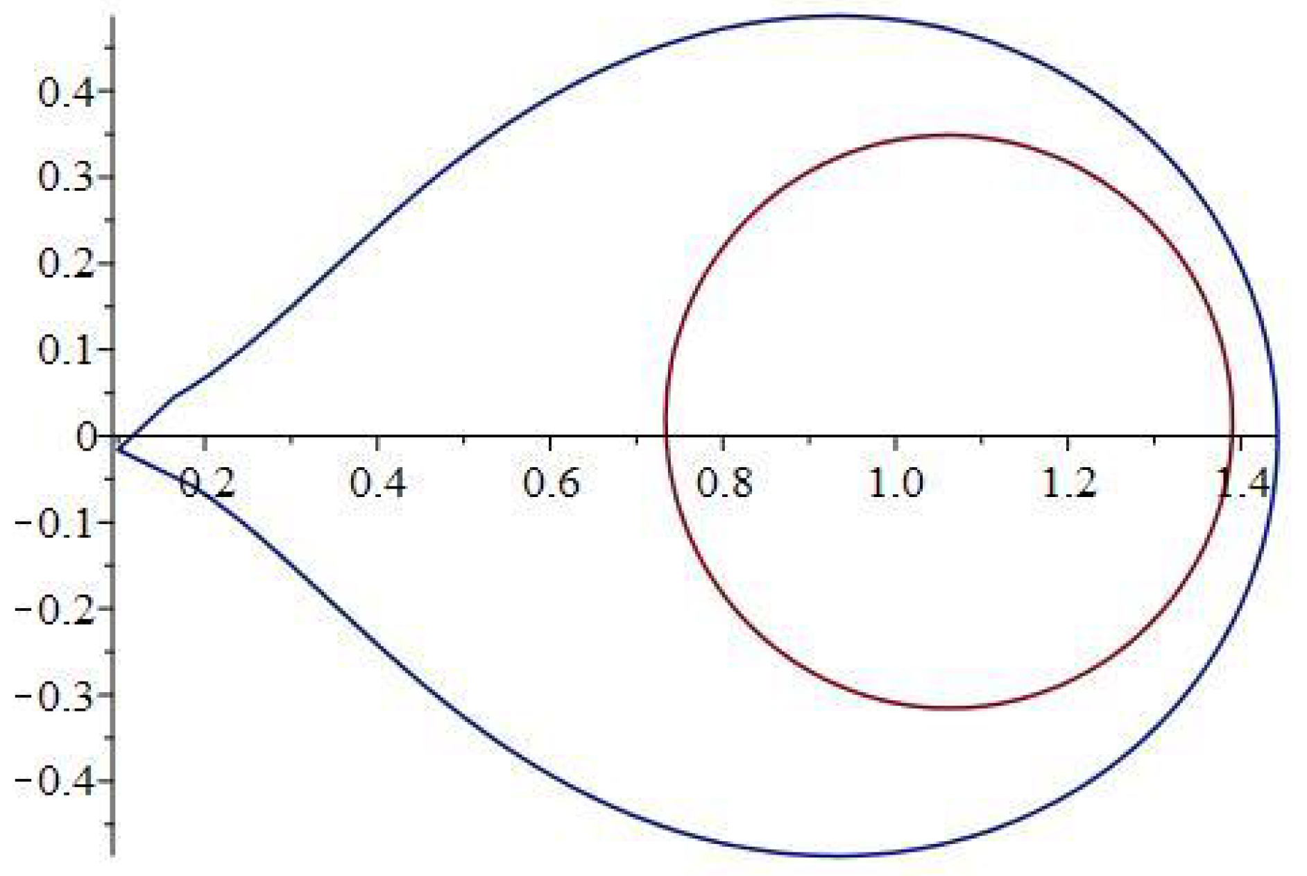
Using the notations of the Definition 3, it is easy to check that $\Theta (-az)=\mathrm{\Lambda }\left(az\right)$ for all $z\in \mathbb{D}$; hence, $\Phi \left(\mathbb{D}\right)=\Psi \left(\mathbb{D}\right)$. Taking the particular case $a=0.12$, $\lambda =\pi /3$, and using the 2D plot of the MAPLE™ computer software, we obtain the image of the boundary $\partial \mathbb{D}$ by the functions Θ, Λ, and $\mathfrak{G}$, presented in Figure 4. Since the function $\mathfrak{G}$ is univalent in $\mathbb{D}$, the subordinations $\Theta \left(z\right)\prec \mathfrak{G}\left(z\right)$ and $\mathrm{\Lambda }\left(w\right)\prec \mathfrak{G}\left(w\right)$ hold because $\Theta \left(0\right)=\mathrm{\Lambda }\left(0\right)=\mathfrak{G}\left(0\right)$, $\Theta \left(\mathbb{D}\right)\subset \mathfrak{G}\left(\mathbb{D}\right)$ and $\mathrm{\Lambda }\left(\mathbb{D}\right)\subset \mathfrak{G}\left(\mathbb{D}\right)$ (see Figure 4). Hence, $f_{*}\in {\mathfrak{G}}_{\Sigma }(\pi /3)$; therefore, the class ${\mathfrak{G}}_{\Sigma }\left(\lambda \right)$ is not empty and contains other functions besides the identity.

In the following theorem, we determine the results for the initial coefficient bounds of the class ${\mathfrak{G}}_{\Sigma }\left(\lambda \right)$.

Theorem 5.

If $f\in {\mathfrak{G}}_{\Sigma }\left(\lambda \right)$ is given by (1), then

$$\left|a_2\right|\le min\left\{\frac{1}{2\left|2+e^{i\lambda }\right|};\sqrt{\frac{3}{2\left|37+20e^{i\lambda }+7e^{2i\lambda }\right|}}\right\},$$

and

$$\left|a_3\right|\le min\left\{\frac{1}{4{\left|2+e^{i\lambda }\right|}^2}+\frac{1}{2\left|5+3e^{i\lambda }\right|};\frac{3}{2\left|37+20e^{i\lambda }+7e^{2i\lambda }\right|}+\frac{1}{2\left|5+3e^{i\lambda }\right|}\right\}.$$

Proof. 

If $f\in {\mathfrak{G}}_{\Sigma }\left(\lambda \right)$, from Definition 3, there exist two analytic functions in $\mathbb{D}$, namely u and v, such that $u\left(0\right)=v\left(0\right)=0$ and $\left|u\right(z\left)\right|<1$, $\left|v\right(w\left)\right|<1$ for all $z,w\in \mathbb{D}$, with

$$\begin{array}{ccc}& & \frac{z{f}^{\prime }\left(z\right)}{f\left(z\right)}+\frac{1+e^{i\lambda }}{2}·\frac{z^2{f}^{\prime \prime }\left(z\right)}{f\left(z\right)}=\mathfrak{G}\left(u\left(z\right)\right),z\in \mathbb{D},\hfill \end{array}$$

(44)

$$\begin{array}{ccc}& & \frac{w{g}^{\prime }\left(w\right)}{g\left(w\right)}+\frac{1+e^{i\lambda }}{2}·\frac{w^2{g}^{\prime \prime }\left(w\right)}{g\left(w\right)}=\mathfrak{G}\left(v\left(w\right)\right),w\in \mathbb{D}.\hfill \end{array}$$

(45)

With the same notations as in the proof of Theorem 3, from the equalities (44) and (45), we obtain that

$$\frac{z{f}^{\prime }\left(z\right)}{f\left(z\right)}+\frac{1+e^{i\lambda }}{2}·\frac{z^2{f}^{\prime \prime }\left(z\right)}{f\left(z\right)}=1+\frac{c_1}{4}z+\frac{1}{48}\left(-7c_1^2+12c_2\right)z^2+\dots ,z\in \mathbb{D},$$

(46)

and

$$\frac{w{g}^{\prime }\left(w\right)}{g\left(w\right)}+\frac{1+e^{i\lambda }}{2}·\frac{w^2{g}^{\prime \prime }\left(w\right)}{g\left(w\right)}=1+\frac{d_1}{4}w+\frac{1}{48}\left(-7d_1^2+12d_2\right)w^2+\dots ,w\in \mathbb{D}.$$

(47)

Equating the corresponding coefficients in (46) and (47), we have

$$\begin{array}{ccc}& & \left(2+e^{i\lambda }\right)a_2=\frac{c_1}{4},\hfill \end{array}$$

(48)

$$\begin{array}{ccc}& & \left(5+3e^{i\lambda }\right)a_3-\left(2+e^{i\lambda }\right)a_2^2=\frac{1}{48}\left(-7c_1^2+12c_2\right),\hfill \end{array}$$

(49)

and

$$\begin{array}{ccc}& & -\left(2+e^{i\lambda }\right)a_2=\frac{d_1}{4},\hfill \end{array}$$

(50)

$$\begin{array}{ccc}& & \left(8+5e^{i\lambda }\right)a_2^2-\left(5+3e^{i\lambda }\right)a_3=\frac{1}{48}\left(-7d_1^2+12d_2\right).\hfill \end{array}$$

(51)

The relations (48) and (50) lead to

$$c_1=-d_1$$

(52)

and

$$32{\left(2+e^{i\lambda }\right)}^2{a}_2^2=c_1^2+d_1^2,$$

i.e.,

$$a_2^2=\frac{c_1^2+d_1^2}{32{\left(2+e^{i\lambda }\right)}^2}.$$

(53)

If we add (49) and (51), we obtain

$$2\left(3+2e^{i\lambda }\right)a_2^2=\frac{1}{4}\left(c_2+d_2\right)-\frac{7}{48}\left(c_1^2+d_1^2\right),$$

(54)

and substituting the value of $\left(c_1^2+d_1^2\right)$ from (53) in the right-hand side of (54), we deduce that

$$\left[2\left(3+2e^{i\lambda }\right)+\frac{14}{3}{\left(2+e^{i\lambda }\right)}^2\right]a_2^2=\frac{1}{4}(c_2+d_2),$$

and thus

$$a_2^2=\frac{3(c_2+d_2)}{4\left[6\left(3+2e^{i\lambda }\right)+14{\left(2+e^{i\lambda }\right)}^2\right]}.$$

(55)

Using (6) of Lemma 1 and the triangle inequality in (53) and (55), we obtain

$$\left|a_2\right|\le \frac{1}{2\left|2+e^{i\lambda }\right|}\mathrm{and}\left|a_2\right|\le \sqrt{\frac{3}{2\left|37+20e^{i\lambda }+7e^{2i\lambda }\right|}},$$

which proves our first inequality.

If we subtract (51) from (49), we obtain

$$2\left(5+3e^{i\lambda }\right)\left(a_3-a_2^2\right)=\frac{c_2-d_2}{4}-\frac{7}{48}\left(c_1^2-d_1^2\right),$$

and in view of (52) and (53), the above relation leads to

$$a_3=a_2^2+\frac{c_2-d_2}{8\left(5+3e^{i\lambda }\right)}=\frac{c_1^2+d_1^2}{32{\left(2+e^{i\lambda }\right)}^2}+\frac{c_2-d_2}{8\left(5+3e^{i\lambda }\right)}.$$

(56)

Using again Lemma 1 and the triangle inequality, it follows that

$$\left|a_3\right|\le \frac{1}{4{\left|2+e^{i\lambda }\right|}^2}+\frac{1}{2\left|5+3e^{i\lambda }\right|}.$$

Similarly, in view of (55) and (52), the relation (56) could be written as

$$a_3=\frac{3(c_2+d_2)}{4\left[6\left(3+2e^{i\lambda }\right)+14{\left(2+e^{i\lambda }\right)}^2\right]}+\frac{c_2-d_2}{8\left(5+3e^{i\lambda }\right)},$$

and from Lemma 1 and the triangle inequality, we conclude that

$$\left|a_3\right|\le \frac{3}{2\left|37+20e^{i\lambda }+7e^{2i\lambda }\right|}+\frac{1}{2\left|5+3e^{i\lambda }\right|},$$

and this proves the second result. □

To determine the upper bound of the Fekete–Szegő functional for the class ${\mathfrak{G}}_{\Sigma }\left(\lambda \right)$, we use the following lemma.

Lemma 3

([24], (3.9), (3.10) p. 254). If $p\left(z\right)=1+c_{1}z+c_2{z}^2+\dots$, $z\in \mathbb{D}$ with $p\in \mathcal{P}$, then there exist some x, ζ with $\left|x\right|\le 1$, $\left|\zeta \right|\le 1$, such that

$$\begin{array}{ccc}& & 2c_2=c_1^2+x\left(4-c_1^2\right),\hfill \\ & & 4c_3=c_1^3+2c_{1}x\left(4-c_1^2\right)-\left(4-c_1^2\right)c_1{x}^2+2\left(4-c_1^2\right)\left(1-{\left|x\right|}^2\right)\zeta .\hfill \end{array}$$

Theorem 6.

If $f\in {\mathfrak{G}}_{\Sigma }\left(\lambda \right)$ is given by (1), then

$$\left|a_3-\rho a_2^2\right|\le \left\{\begin{array}{cc}{\displaystyle \frac{1}{2\left|5+3e^{i\lambda }\right|}},\hfill & for|1-\rho |\le {\displaystyle \frac{4{\left|2+e^{i\lambda }\right|}^2}{3\left|5+3e^{i\lambda }\right|}},\hfill \\ {\displaystyle \frac{|1-\rho |}{4{\left|2+e^{i\lambda }\right|}^2}},\hfill & for|1-\rho |\ge {\displaystyle \frac{4{\left|2+e^{i\lambda }\right|}^2}{3\left|5+3e^{i\lambda }\right|}}.\hfill \end{array}\right.$$

(57)

Proof. 

If $f\in {\mathfrak{G}}_{\Sigma }\left(\lambda \right)$ has the form (1), using (52) and (53), we have $a_2^2={\displaystyle \frac{c_1^2}{16{\left(2+e^{i\lambda }\right)}^2}}$. Thus, from (55) and (56), we obtain

$$a_3-\rho a_2^2=(1-\rho )\frac{c_1^2}{16{\left(2+e^{i\lambda }\right)}^2}+\frac{c_2-d_2}{8(5+3e^{i\lambda })}.$$

With the same notations as in the proof of Theorem 3, from Lemma 3, we have $2c_2=c_1^2+x\left(4-c_1^2\right)$ and $2d_2=d_1^2+y(4-d_1^2)$, $\left|x\right|\le 1$, $\left|y\right|\le 1$, and using (52), we obtain

$$c_2-d_2=\frac{4-c_1^2}{2}(x-y),$$

and thus

$$a_3-\rho a_2^2=(1-\rho )\frac{c_1^2}{16{\left(2+e^{i\lambda }\right)}^2}+\frac{\left(4-c_1^2\right)(x-y)}{16(5+3e^{i\lambda })}.$$

From the triangle inequality, taking $\left|x\right|=\delta$, $\left|y\right|=\kappa$, $\delta ,\kappa \in [0,1]$, and without losing generality, we can assume that $c_1\in \mathbb{R}$, $c_1=t\in [0,2]$; thus, we obtain

$$|a_3-\rho a_2^2|\le |1-\rho |\frac{t^2}{16{\left|2+e^{i\lambda }\right|}^2}+\frac{1}{16\left|5+3e^{i\lambda }\right|}(4-t^2)(\delta +\kappa ).$$

Denoting $\mathcal{M}\left(t\right):={\displaystyle \frac{|1-\rho |t^2}{16{\left|2+e^{i\lambda }\right|}^2}}\ge 0$ and $\mathcal{N}\left(t\right):={\displaystyle \frac{4-t^2}{16\left|5+3e^{i\lambda }\right|}}\ge 0$, the above relation can be rewritten in the form

$$|a_3-\rho a_2^2| \le \mathcal{M}\left(t\right)+\mathcal{N}\left(t\right)(\delta +\kappa )=:\mathcal{Y}(\delta ,\kappa ),\delta ,\kappa \in [0,1].$$

Therefore,

$$max\left\{\mathcal{Y}(\delta ,\kappa ):\delta ,\kappa \in [0,1]\right\}=\mathcal{Y}(1,1)=\mathcal{M}\left(t\right)+2\mathcal{N}\left(t\right)=:H\left(t\right),t\in [0,2]$$

and substituting the value $\mathcal{M}\left(t\right)$ and $\mathcal{N}\left(t\right)$ in the above equality, we obtain

$$H\left(t\right)=\frac{1}{16{\left|2+e^{i\lambda }\right|}^2}\left(|1-\rho |-\frac{2{\left|2+e^{i\lambda }\right|}^2}{\left|5+3e^{i\lambda }\right|}\right)t^2+\frac{1}{2\left|5+3e^{i\lambda }\right|}.$$

Next we will determine the maximum of H on $[0,2]$. Since

$$H^{\prime }\left(t\right)=\frac{1}{8{\left|2+e^{i\lambda }\right|}^2}\left(|1-\rho |-2\frac{{\left|2+e^{i\lambda }\right|}^2}{\left|5+3e^{i\lambda }\right|}\right)t,$$

it is clear that $H^{\prime }\left(t\right)\le 0$ if and only if $|1-\rho |\le {\displaystyle \frac{2{\left|2+e^{i\lambda }\right|}^2}{\left|5+3e^{i\lambda }\right|}}$. In this case, function H is a decreasing function on $[0,2]$; therefore,

$$max\left\{H\left(t\right):t\in [0,2]\right\}=H\left(0\right)=\frac{1}{2\left|5+3e^{i\lambda }\right|}.$$

It is easy to check that $H^{\prime }\left(t\right)\ge 0$ if and only if $|1-\rho |\ge {\displaystyle \frac{2{\left|2+e^{i\lambda }\right|}^2}{\left|5+3e^{i\lambda }\right|}}$; hence, the function H is an increasing function on $[0,2]$, and consequently

$$max\left\{H\left(t\right):t\in [0,2]\right\}=H\left(2\right)=\frac{|1-\rho |}{4{\left|2+e^{i\lambda }\right|}^2},$$

and the estimation (57) is proven. □

5. Conclusions

In our present investigation, we have introduced and studied the initial coefficient problems associated with each of the new subclasses ${\mathfrak{HG}}_{\Sigma }$, ${\mathfrak{M}}_{\Sigma }\left(\tau \right)$ and ${\mathfrak{G}}_{\Sigma }\left(\lambda \right)$ of the well-known bi-univalent class $\Sigma$. These bi-univalent function subclasses are given by Definitions 1–3, respectively. For the functions in each of these bi-univalent subclasses, we have obtained an improvement in the estimates of the Taylor–Maclaurin coefficients $\left|a_2\right|$ and $\left|a_3\right|$, and we have given solutions for the Fekete–Szegő functional problems. New results are shown to follow upon specializing the parameters involved in our main results, as given in Remark 2 for the class of bi-starlike and bi-convex functions associated with Gregory coefficients, which are new and have not been studied so far. Further, we can extend these types of studies based on generalized telephone numbers (see [25,26,27]).