Abstract
This article studies diverse forms of lump-type solutions for coupled nonlinear generalized Zakharov equations (CNL-GZEs) in plasma physics through an appropriate transformation approach and bilinear equations. By utilizing the positive quadratic assumption in the bilinear equation, the lump-type solutions are derived. Similarly, by employing a single exponential transformation in the bilinear equation, the lump one-soliton solutions are derived. Furthermore, by choosing the double exponential ansatz in the bilinear equation, the lump two-soliton solutions are found. Interaction behaviors are observed and we also establish a few new solutions in various dimensions (3D and contour). Furthermore, we compute rogue-wave solutions and lump periodic solutions by employing proper hyperbolic and trigonometric functions.
MSC:
35J05; 35J10; 35K05; 35L05
1. Introduction
The study of partial differential equations (PDEs) occurs in various fields such as theoretical physics, applied mathematics, biological sciences, and engineering sciences. These PDEs play a crucial role in explaining key scientific phenomena. For instance, the Korteweg–de Vries equation governs shallow water wave dynamics near ocean shores and beaches, and the nonlinear Schrödinger’s equation governs the propagation of solitons through optical fibers. Some examples of PDEs and their applications can be found in [1,2,3,4,5,6,7,8].
Although the above-mentioned PDEs are scalar, a large number of PDEs are coupled. Some of them are two-coupled PDEs such as the Gear–Grimshaw equation, whereas others are three-coupled PDEs. An example of a three-coupled PDE is the Wu–Zhang equation. These coupled PDEs are also calculated in distinct areas of theoretical physics. In this paper, we will study CNL-GZE used in plasmas.
Lump waves (LWs), as superior nonlinear wave phenomena, have been visualized in various fields. LWs are theoretically viewed as a limited type of soliton and move with higher propagating energy compared to general solitons. Consequently, LWs can be destructive and even catastrophic in certain systems, such as in the ocean and finance. It is important to be able to find and anticipate LWs in practical applications. In recent years, studies on lump solutions have increased, leading to more specialized investigations. Therefore, theoretical investigations of LWs are instrumental in enhancing our understanding and predicting possible extremes in nonlinear systems [9,10,11,12,13].
Finding the lump solutions of PDEs has become a primary focus in recent years. As a result, several mathematical experts have developed important schemes in order to solve PDEs [14,15,16].
In this article, we consider the CNL-GZE for the complex envelope of the high-frequency wave and the real low-frequency field , as follows [17]:
where and are real constants. The cubic term in Equation (1) represents the nonlinear self-interaction in the high-frequency subsystem, which corresponds to a self-focusing effect in plasma physics.
Several researchers have worked on the stated model. For instance, Wang et al. evaluated periodic wave solutions for GZEs using the extended F-expansion method [17]. Zheng et al. performed a numerical simulation of a GZ system [18]. Bao et al. developed numerical schemes for a GZ system [19]. Bhrawy et al. constructed an efficient Jacobi pseudospectral approximation for a nonlinear complex GZ system [20]. Zhang et al. studied solitary wave solutions through a variational approach [21]. Similarly, Yildirim et al. studied some newly discovered soliton solutions of GZEs by applying He’s variational approach [22]. Li et al. computed additional exact solutions of GZEs through the Exp-function method [23]. Buhe et al. studied symmetry reductions, conservation laws, and exact solutions for GZEs [24]. Lin et al. constructed some additional exact solutions for GZEs through the Exp-function method [23]. Wu et al. studied exact solutions for GZEs using a variational approach [25]. However, in this paper, we will explore lump, lump-type, lump one-strip, and lump two-strip solutions for CNL-GZEs through appropriate transformation methods and bilinear equations. We compute the lump solutions by choosing the appropriate polynomial function. In addition, we compute lump-periodic and rogue-wave solutions by using logarithmic transformation.
This article is organized as follows. In Section 2, we form bilinear equations and evaluate lump solutions for the coupled nonlinear generalized Zakharov equations in plasma physics through appropriate transformation approaches. The solutions are presented along with with their corresponding graphs. The mixed solutions of soliton and lump waves are provided in Section 3. We evaluate the lump one-strip and lump two-strip solutions using suitable profiles in Section 3. By employing a trigonometric ansatz in the bilinear equation, we compute lump periodic solutions in Section 4. By utilizing a hyperbolic ansatz in the bilinear equation, we explore rogue-wave solutions in Section 5. Section 6 discusses the results of the obtained solutions, and finally, in Section 7, we present some concluding remarks.
2. Lump Solution
For the lump solutions of Equation (1), we apply the following ansatz: [26,27,28,29,30],
then, we obtain the bilinear equations,
and
respectively.
Now, to obtain the LP solution, the functions p and q in Equations (3) and (4) are assumed to be [27,28],
where ,
In addition, are specific constants. Now, by substituting Equation (5) into Equations (3) and (4) and solving the equations obtained from the coefficients of x and t, we obtain:
Set I. The values of unknowns for Equations (3) and (4), respectively, are as follows:
Then, the values in Equation (6) generate the required solutions for Equations (3) and (4), which are, respectively,
and
Set II. The values of the parameters in Equations (3) and (4) are, respectively,
Then, the values in Equation (9) generate the required solutions for Equations (3) and (4), which are, respectively,
and
3. Mixed Solutions of Soliton and Lump Waves
In this section, we study the interaction of a lump soliton with a single kink wave and the interaction of a lump soliton with double kink waves.
3.1. Lump One-Strip Soliton Interaction Solution
To obtain the lump one-strip solution, we use the transformations given in Equations (3) and (4) [22,27,28,29,30]:
where , , and , , and are any constants. Now, from Equations (12) and (4), we obtain the coefficients of x and t and solve the equations as follows:
Set I. The values of the parameters in Equations (3) and (4) are, respectively,
Then, the values in Equation (13) generate the required results for Equations (3) and (4), which are, respectively,
and
Set II. The values of the parameters in Equations (3) and (4) are, respectively,
Then, the values in Equation (16) generate the required results for Equations (3) and (4), which are, respectively,
and
3.2. Lump Double-Strip Soliton Interaction Solution
To obtain the lump two-strip solution, we assume the following transformation [22,27,28,29,30]:
where , , and , , , and are specific real parameters. Now, from Equation (19) and Equation (4), we obtain the coefficients of x, t, and and solve these equations as follows:
Then, the values in Equation (20) generate the required results for Equations (3) and (4), which are, respectively,
and
Then, the values in Equation (23) generate the required results for Equations (3) and (4), which are, respectively,
and
4. Lump Periodic Soliton Solution
To compute the LPS solution, we use the following supposition in Equations (3) and (4) [22,27,28,29,30]:
where , . In addition, and are various parameters to be determined. Now, by substituting Equation (26) into Equations (3) and (4) and then examining the coefficients of x, cos function, and t, we obtain the following:
Set I. The values of the parameters for Equations (3) and (4) are, respectively,
Then, the values in Equation (27) generate the required results for Equations (3) and (4), which are, respectively,
and
5. Rogue-Wave Solutions
To compute the LPS solution, we use the following supposition in Equations (3) and (4) [22,27,28,29,30]:
where , In addition, and are various parameters to be determined. Now, by substituting Equation (26) into Equations (3) and (4) and then examining the coefficients of x, cos function, and t, we obtain the following:
Set I. The values of the parameters for Equations (3) and (4), are, respectively,
Then, the values in Equation (31) generate the solutions for Equations (3) and (4), which are, respectively,
and
6. Results and Discussion
We observed that the solution in Equation (7) with and formed two lump waves (LWs) known as upper-bright and lower-dark LWs, and that the bright and dark LWs were symmetrical about the coordinate plane. As varied from a minimum to a maximum number, the two LWs rotated counterclockwise. When , the LW disappeared, but at , the LW gradually reappeared (see Figure 1). The contour lump-wave profiles for are plotted for and in Figure 2. The mixed solutions of soliton and lump waves were successfully obtained. Notice that our solution in Equation (14) with and formed lump one-strip waves (LSWs) known as upper-bright LSWs. The lump one-strip wave profiles for are depicted for and in Figure 3 and Figure 4. The lump double-strip wave profiles for are plotted for and in Figure 3, Figure 5 and Figure 6. By utilizing the assumption of the cosine function in bilinear equations in Equations (3) and (4), we have obtained the lump periodic solutions. We have successfully obtained the lump periodic graphs for , which are plotted for and in Figure 7. The lump periodic contour graphs for are plotted for and in Figure 8. By utilizing the assumption of cosine hyperbolic functions in bilinear equations in Equations (3) and (4), we have obtained the lump periodic solutions. As varied from −10 to 10, the rogue wave rotated, and its behavior can be seen for for and in Figure 9.
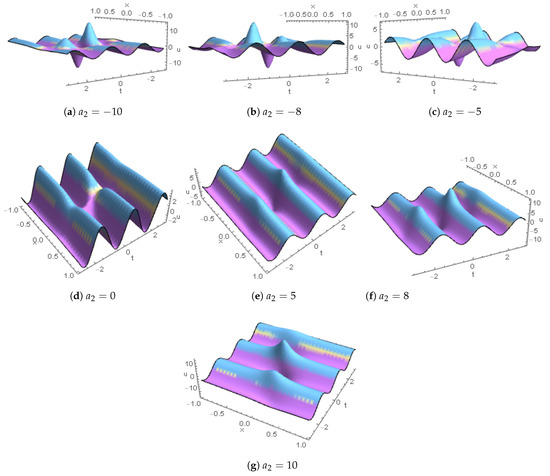
Figure 1.
Lump-wave profiles for are plotted for .
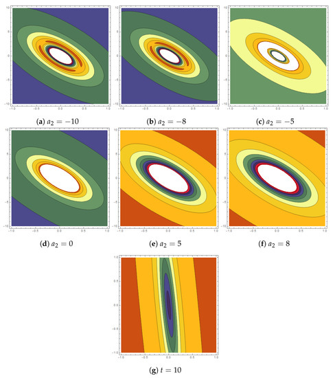
Figure 2.
Contour lump-wave profiles for are plotted for .

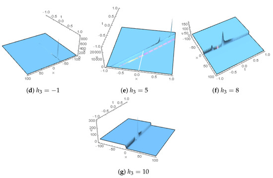
Figure 3.
Lump one-strip wave profiles for are plotted for .
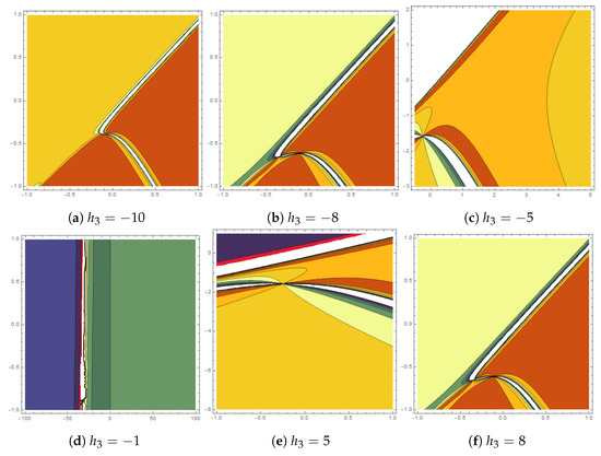
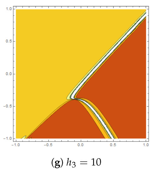
Figure 4.
Contour lump one-strip wave profiles for are plotted for .
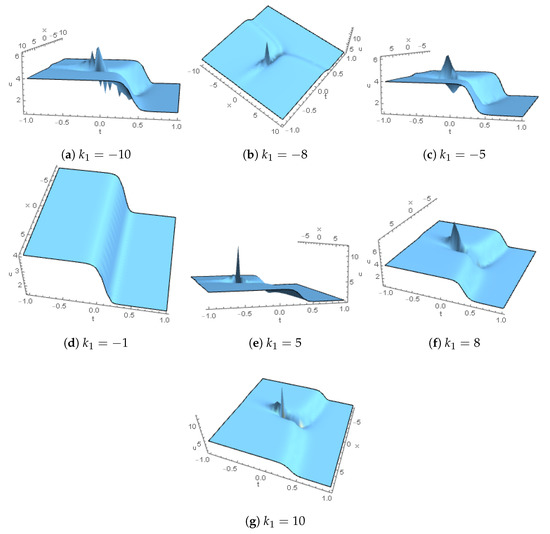
Figure 5.
Lump double-strip wave profiles for are plotted for .
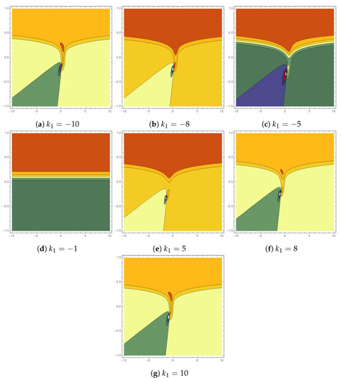
Figure 6.
Contour profiles for Figure 5.
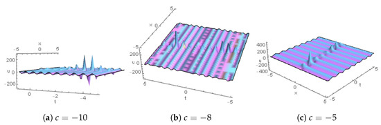
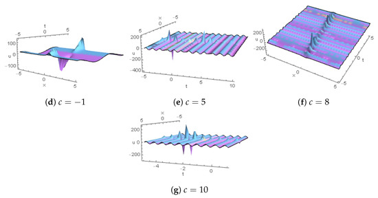
Figure 7.
Lump periodic graphs for are plotted for .
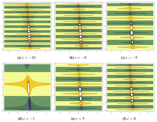
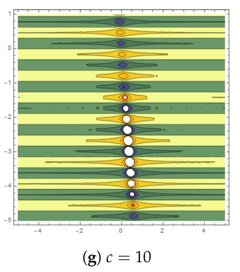
Figure 8.
Lump periodic contour graphs for are plotted for .
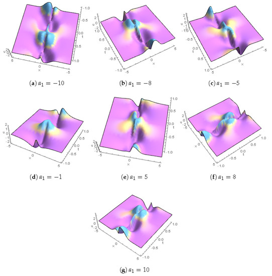
Figure 9.
Rogue-wave profiles for are plotted for .
7. Concluding Remarks
In this paper, we have studied multiple forms of lump solutions for CNL-GZEs in plasma physics using appropriate transformation approaches, bilinear equations, and symbolic computations. By utilizing the positive quadratic assumption in the bilinear equation, we have derived the lump-type solutions. We have evaluated the lump one-soliton solutions through a single exponential function transformation in the bilinear equation. Similarly, we have computed the lump two-soliton solutions using a double exponential function transformation in the bilinear equation. Mixed solutions of lump waves and solitons have been successfully evaluated. Furthermore, we have computed rogue-wave solutions and lump periodic solutions by utilizing appropriate hyperbolic and trigonometric functions. We have identified certain constraint values throughout the derivation of the solutions that must hold for the soliton solution to exist. The presented solutions have valuable uses in plasma physics.
Author Contributions
Methodology, Methodology and Writing—review & editing, S.T.R.R.; Formal analysis, H.Z.; Supervision, A.R.S. All authors have read and agreed to the published version of the manuscript.
Funding
The Deputyship for Research and Innovation in the Ministry of Education in Saudi Arabia for funding this research work under project number 141/442.
Data Availability Statement
Not applicable.
Acknowledgments
The authors extend their appreciation to the Deputyship for Research and Innovation in the Ministry of Education in Saudi Arabia for funding this research work under project number 141/442. Furthermore, the authors would like to extend their appreciation to Taibah University for its supervisory support.
Conflicts of Interest
The authors declare no conflict of interest.
References
- Ahmed, S.; Seadawy, A.R.; Rizvi, S.T. Study of breathers, rogue waves and lump solutions for the nonlinear chains of atoms. Opt. Quantum Electron. 2022, 54, 320. [Google Scholar] [CrossRef]
- Ding, Q.; Wong, P.J. A higher order numerical scheme for solving fractional Bagley-Torvik equation. Math. Methods Appl. Sci. 2022, 45, 1241–1258. [Google Scholar] [CrossRef]
- Seadawy, A.R.; Rizvi, S.T.; Ahmed, S. Weierstrass and Jacobi elliptic, bell and kink type, lumps, Ma and Kuznetsov breathers with rogue wave solutions to the dissipative nonlinear Schrödinger equation. Chaos Solitons Fractals 2022, 160, 112258. [Google Scholar] [CrossRef]
- Seadawy, A.R.; Ahmed, S.; Rizvi, S.T.; Ali, K. Various forms of lumps and interaction solutions to generalized Vakhnenko Parkes equation arising from high-frequency wave propagation in electromagnetic physics. J. Geom. Phys. 2022, 176, 104507. [Google Scholar] [CrossRef]
- Seadawy, A.R.; Ahmed, S.; Rizvi, S.T.; Ali, K. Lumps, breathers, interactions and rogue wave solutions for a stochastic gene evolution in double chain deoxyribonucleic acid system. Chaos Solitons Fractals 2022, 161, 112307. [Google Scholar] [CrossRef]
- Seadawy, A.R.; Rizvi, S.T.; Ahmed, S. Multiple lump, generalized breathers, Akhmediev breather, manifold periodic and rogue wave solutions for generalized Fitzhugh-Nagumo equation: Applications in nuclear reactor theory. Chaos Solitons Fractals 2022, 161, 112326. [Google Scholar] [CrossRef]
- Seadawy, A.R.; Rizvi, S.T.; Ahmed, S.; Younas, M. Applications of lump and interaction soliton solutions to the Model of liquid crystals and nerve fibers. Encycl. Complex. Syst. Sci. 2022, 1–20. [Google Scholar]
- Bashir, A.; Seadawy, A.R.; Ahmed, S.; Rizvi, S.T. The Weierstrass and Jacobi elliptic solutions along with multiwave, homoclinic breather, kink-periodic-cross rational and other solitary wave solutions to Fornberg Whitham equation. Chaos Solitons Fractals 2022, 163, 112538. [Google Scholar] [CrossRef]
- Seadawy, A.R.; Rizvi, S.T.R.; Ahmad, S.; Younis, M.; Baleanu, D. Lump, lump-one stripe, multiwave and breather solutions for the Hunter–Saxton equation. Open Phys. 2021, 19, 1–10. [Google Scholar] [CrossRef]
- Li, X.; Wong, P.J. Generalized Alikhanov’s approximation and numerical treatment of generalized fractional sub-diffusion equations. Commun. Nonlinear Sci. Numer. Simul. 2021, 97, 105719. [Google Scholar] [CrossRef]
- Ahmad, H.; Seadawy, A.R.; Khan, T.A. Numerical Solution of Korteweg-de Vries-Burgers Equation by the Modified Variational Iteration Algorithm-II arising in shallow water waves. Phys. Scr. 2020, 95, 45210. [Google Scholar] [CrossRef]
- Li, X.; Wong, P.J. gL1 Scheme for Solving a Class of Generalized Time-Fractional Diffusion Equations. Mathematics 2022, 10, 1219. [Google Scholar] [CrossRef]
- Soundararajan, R.; Subburayan, V.; Wong, P.J. Streamline Diffusion Finite Element Method for Singularly Perturbed 1D-Parabolic Convection Diffusion Differential Equations with Line Discontinuous Source. Mathematics 2023, 11, 2034. [Google Scholar] [CrossRef]
- Liu, Y.; Li, B.; Wazwaz, A.M. Novel high-order breathers and rogue waves in the Boussinesq equation via determinants. Int. J. Mod. Phys. 2020, 43, 3701–3715. [Google Scholar] [CrossRef]
- Younas, U.; Seadawy, A.R.; Younis, M.; Rizvi, S.T.R. Optical solitons and closed form solutions to (3+1)-dimensional resonant Schrodinger equation. Int. J. Mod. Phys. 2020, 34, 2050291. [Google Scholar] [CrossRef]
- Ghaffar, A.; Ali, A.; Ahmed, S.; Akram, S.; Baleanu, D.; Nisar, K.S. A novel analytical technique to obtain the solitary solutions for nonlinear evolution equation of fractional order. Adv. Differ. Equ. 2020, 1, 308. [Google Scholar] [CrossRef]
- Wang, M.; Li, X. Extended F-expansion method and periodic wave solutions for the generalized Zakharov equations. Phys. Lett. A 2005, 343, 48–54. [Google Scholar] [CrossRef]
- Jin, S.; Markowich, P.A.; Zheng, C. Numerical simulation of a generalized Zakharov system. J. Comput. Phys. 2004, 201, 376–395. [Google Scholar] [CrossRef]
- Bao, W.; Sun, F.; Wei, G.W. Numerical methods for the generalized Zakharov system. J. Comput. Phys. 2003, 190, 201–228. [Google Scholar] [CrossRef]
- Bhrawy, A.H. An efficient Jacobi pseudospectral approximation for nonlinear complex generalized Zakharov system. Appl. Math. Comput. 2014, 247, 30–46. [Google Scholar] [CrossRef]
- Zhang, J. Variational approach to solitary wave solution of the generalized Zakharov equation. Comput. Math. Appl. 2007, 54, 1043–1046. [Google Scholar] [CrossRef]
- Khan, Y.; Faraz, N.; Yildirim, A. New soliton solutions of the generalized Zakharov equations using He’s variational approach. Appl. Math. Lett. 2011, 24, 965–968. [Google Scholar] [CrossRef]
- Li, Y.Z.; Li, K.M.; Lin, C. Exp-function method for solving the generalized-Zakharov equations. Appl. Math. Comput. 2008, 205, 197–201. [Google Scholar] [CrossRef]
- Buhe, E.; Bluman, G.W. Symmetry reductions, exact solutions, and conservation laws of the generalized Zakharov equations. J. Math. Phys. 2015, 56, 101501. [Google Scholar] [CrossRef]
- Wu, Y. Variational approach to the generalized Zakharov equations. Int. J. Nonlinear Sci. Numer. Simul. 2009, 10, 1245–1248. [Google Scholar] [CrossRef]
- Seadawy, A.R.; Rizvi, S.T.; Ashraf, M.A.; Younis, M.; Hanif, M. Rational solutions and their interactions with kink and periodic waves for a nonlinear dynamical phenomenon. Int. J. Mod. Phys. B 2021, 35, 2150236. [Google Scholar] [CrossRef]
- Wang, H. Lump and interaction solutions to the (2+1)-dimensional Burgers equation. Appl. Math. Lett. 2018, 85, 27–34. [Google Scholar] [CrossRef]
- Zhou, Y.; Manukure, S.; Ma, W.X. Lump and lump-soliton solutions to the Hirota Satsuma equation. Commun. Nonlinear Sci. Numer. Simul. 2019, 68, 56–62. [Google Scholar] [CrossRef]
- Wu, P.; Zhang, Y.; Muhammad, I.; Yin, Q. Lump, periodic lump and interaction lump stripe solutions to the (2+1)-dimensional B-type Kadomtsev–Petviashvili equation. Mod. Phys. Lett. B 2018, 32, 1850106. [Google Scholar] [CrossRef]
- Li, B.Q.; Ma, Y.L. multiple-lump waves for a (3+1)-dimensional Boiti–Leon–Manna–Pempinelli equation arising from incompressible fluid. Comput. Math. Appl. 2018, 76, 204–214. [Google Scholar] [CrossRef]
Disclaimer/Publisher’s Note: The statements, opinions and data contained in all publications are solely those of the individual author(s) and contributor(s) and not of MDPI and/or the editor(s). MDPI and/or the editor(s) disclaim responsibility for any injury to people or property resulting from any ideas, methods, instructions or products referred to in the content. |
© 2023 by the authors. Licensee MDPI, Basel, Switzerland. This article is an open access article distributed under the terms and conditions of the Creative Commons Attribution (CC BY) license (https://creativecommons.org/licenses/by/4.0/).