Sparse Support Tensor Machine with Scaled Kernel Functions

Abstract

As one of the supervised tensor learning methods, the support tensor machine (STM) for tensorial data classification is receiving increasing attention in machine learning and related applications, including remote sensing imaging, video processing, fault diagnosis, etc. Existing STM approaches lack consideration for support tensors in terms of data reduction. To address this deficiency, we built a novel sparse STM model to control the number of support tensors in the binary classification of tensorial data. The sparsity is imposed on the dual variables in the context of the feature space, which facilitates the nonlinear classification with kernel tricks, such as the widely used Gaussian RBF kernel. To alleviate the local risk associated with the constant width in the tensor Gaussian RBF kernel, we propose a two-stage classification approach; in the second stage, we advocate for a scaling strategy on the kernel function in a data-dependent way, using the information of the support tensors obtained from the first stage. The essential optimization models in both stages share the same type, which is non-convex and discontinuous, due to the sparsity constraint. To resolve the computational challenge, a subspace Newton method is tailored for the sparsity-constrained optimization for effective computation with local convergence. Numerical experiments were conducted on real datasets, and the numerical results demonstrate the effectiveness of our proposed two-stage sparse STM approach in terms of classification accuracy, compared with the state-of-the-art binary classification approaches.

1. Introduction

Tensors, also known as multi-way arrays, are ubiquitous in the big data era, with applications distributed in brain imaging, video surveillance, hyperspectral images, measurements in social networks, climatology, and geography [1]. Multilinear structures in tensorial data allow for the effective capture of spatial characteristics and intrinsic dimension-reduced properties, instead of working on flattened vectors. Tensor-based thinking has emerged in data mining and machine learning. While the development of theory and algorithms for tensor decompositions [2] has garnered extensive attention due to successful applications in unsupervised learning, supervised tensor learning (STL) methods have also received praise in various fields, including remote sensing imaging [3,4], video processing [5,6], fault diagnosis [7,8], and so on. Pioneering work can be traced back to Tao et al. [9], where the support vector machine (SVM) and minimax probability machine (MPM) were generalized to rank-one tensors for tensorial data classification. Sequential works on binary classification for tensors, namely STM, were delivered in [10,11,12,13,14] and the references therein. Related classification models in tensor format can be found in the one-class STM [15], twin STM  [16,17,18], etc. In the literature on tensor classification, a common assumption imposed on the underlying weight tensor, which contributes to the decision function, is low-rankness. It provides advantages in alleviating overfitting issues for small sample-sized problems [19,20] since the dimensions of the weight tensor to be learned are substantially larger than the sample size in practice. The tensor rank notion is far more complicated than the matrix rank, leading to statistical and computational challenges. Another major difficulty in STM is how to build predictive models that can leverage the multi-dimensional structures of tensorial data to facilitate the learning process. Previous works concentrated on linear models, where the data were assumed to be linearly separable in the input space [10,11,13,21,22]. However, this assumption is often violated in practical problems and the linear decision boundaries are not adequate to classify the data appropriately [23]. Inspired by the success of kernel tricks in the conventional SVM, it was witnessed in [24,25,26,27,28] that the classification accuracy can be greatly improved by combining tensor decompositions with kernel-based methods. For example, the dual structure-preserving kernel (DuSK) proposed by He et al. [24] was constructed by feeding the factor vectors from the tensor CANDECOM/PARAFAC (CP) decomposition with the conventional Gaussian RBF kernel. As one of the most commonly used kernels, the Gaussian RBF kernel with a constant kernel width may bring about some local risks and short flexibilities in the distance metric, especially when dealing with unevenness in the pattern space. To address this issue, the scaling technique that conformally modifies the kernels (following the principles of Riemannian geometry [29]) was advocated in the settings of kernelized SVMs in [30,31,32,33,34]. A two-stage method is proposed to improve the classification performance, where a primal kernel is used to find the locations of support vectors in the first stage of learning, and the scaled kernel, based on the prior information on support vectors, is constructed to contribute to a better nonlinear classifier. Although the Gaussian RBF kernel is popular with STMs for obtaining the nonlinear boundaries, there is a lack of consideration regarding the local risk caused by using a constant width for tensorial classification. The enhanced learning process on SVMs has motivated us to use a similar technique in the training process for STM.

In this paper, to develop an efficient classification method, we focus on an STM model with the piecewise quadratic smooth loss, which makes the dual problem somewhat more tractable. To reduce the local risk associated with the constant width of the tensor Gaussian RBF kernel, we scaled the kernel function in the training process. Since the scaling kernel depends on support tensor information, we incorporated a sparsity constraint on the support tensors to reduce redundant information in the training process. The idea of sparsity is analogous to the sparse linearly kernelized SVM proposed by Zhou [35], where the proposed classification method has shown superiority in both computation speed and classification accuracy. To the best of our knowledge, this will be the first attempt that considers the sparsity of support tensors for STM. To conclude, we summarize the main contributions of this paper as follows:

• Sparse-kernelized STM model: Taking the sparsity of support tensors into consideration, the sparse-kernelized STM model is proposed, which can flexibly govern the number of support tensors through sparsity constraints. Moreover, the Gaussian RBF kernel in combination with tensor decomposition was utilized to handle nonlinearly separable tensor data.
• Scaled kernel function: To alleviate the local risk caused by the constant kernel width, we modified the kernel through conformal transformation by exploiting the structure of Riemannian geometry induced by the kernel function.
• Two-stage method: The scaling kernel function can be realized via a two-stage training process. In the first stage, we obtained prior information on support tensors by utilizing a primal kernel. Then, the scaled kernel was used to obtain the final classifier in the second stage. Leveraging the sparse structure, we applied the subspace Newton method to solve the optimization problems in both stages.

To clarify our proposed classification approach, we provide a detailed flowchart in Figure 1. The remaining parts of this paper are organized as follows. In Section 2, related works are reviewed. In Section 3, we introduce some tensor basics. In Section 4, the proposed sparse-kernelized STM model is built and a two-stage training process is designed with scaled tensor kernels. In Section 5, the numerical experiments based on real datasets are constructed to validate the superiority of the proposed algorithm. The conclusions are drawn in Section 6.

2. Related Works

With different predictive models assumed in binary classification problems using the tensor-based large margin classification paradigm, the existing works on STM can be simply divided into two categories: linear STM and nonlinear STM with kernels. With linear models, which assume that samples are linearly separable in the input space, the classification approach initially referred to as the STM with the weight tensor as a rank-one tensor was proposed by Tao et al. [10]. It was solved through the alternating projection optimization method, where the expressive power was limited by the rank-one assumption. To retain more structural information from samples, the rank-one weight tensor was replaced with a rank-R $(R>1)$ tensor based on CP decomposition, as described in [21]. Together with the Tucker decomposition, Kotsia [11] developed a support Tucker machine (STuM), where the weight parameter was represented by the Tucker tensor. Along with the CP and Tucker representations, Chen et al. [13] proposed the support tensor train machine (STTM) based on tensor train (TT) decomposition. Going further into the general tensor low-rank constraint (with no reduction of parameters), Wang et al. [36] proposed the low-rank STM based on the ${\mathcal{L}}_{0/1}$ soft-margin loss function. Lian [37] employed the multilinear nuclear norm regularization to construct STM and analyzed its oracle properties. This idea of using a surrogate for tensor decomposition is analogous to what is proposed in [22,38]. The aforementioned works mainly focused on linearly separable tensor data, which are impractical for linear decision boundaries to suit real data in numerous practical applications [23].

Recently, the existing approaches have verified that it is useful to exploit the tensor structure with nonlinear kernels. He et al. [24] combined CP decomposition with kernel tricks and proposed the so-called DuSK to exploit discriminative nonlinear relationships among tensorial data. A similar idea was implemented in [25,39]. In particular, the linear support higher-order tensor machine (SHTM) [40] is deemed as a special case of DuSK. The structural-preserving scheme in the CP-based DuSK was extended to that under TT and TR decompositions [26,27,28]. A summarization of the aforementioned works can be found in

Table 1. Some related works on STM.

	Kernel (Scaled)	Loss	LRD	SST	DR
Tao et al. [10]	× (×)	hinge	CP	×	✓
Kotsia et al. [11]	× (×)	hinge	Tucker	×	✓
Kotsia et al. [21]	× (×)	hinge	CP	×	✓
Yang et al. [22]	× (×)	hinge	×	×	×
Chen et al. [13]	× (×)	hinge	TT	×	✓
Shu et al. [38]	×(×)	hinge	×	×	×
Wang et al. [36]	× (×)	0/1 loss	×	×	×
Hao et al. [40]	linear(×)	hinge	CP	×	✓
He et al. [24]	RBF(×)	hinge	CP	×	✓
He et al. [25]	RBF(×)	hinge	CP	×	✓
Chen et al. [26]	RBF(×)	hinge	TT	×	✓
Kour et al. [27]	RBF(×)	hinge	TT	×	✓
Deng et al. [28]	RBF (×)	hinge	TR	×	✓
Our work	RBF (✓)	piecewise quadratic smooth loss	CP	×	×

, where the “Loss” column presents the loss functions in STMs, “LRD” represents the low-rank decomposition type, “SST” is short for the sparsity of support tensors, and “DR” indicates data reduction.

As one can see from Table 1, among the linear and nonlinear STMs, the hinge loss (i.e., the convex relaxation for the $0/1$ loss that counts the number of misclassified samples) is employed in most of the STM models, except in [36]. As mentioned in the introduction, the low-rank approximation based on tensor decompositions is used for dimension reduction, with three exceptions in [22,36,38], where the original weight tensor is the decision variable with a tensor rank constraint in the underlying optimization model. The data reduction in the existing two-class STMs is due to the tensor decomposition rather than the sparsity constraint on the support tensors. In all kernelized STMs, the scaled scheme on the kernel function is not considered. All of this motivated us to consider the sparse STM with scaled kernels in this paper. As mentioned by Zhou in [35], the piecewise quadratic smooth loss function ${\mathit{\ell }}_{cC}(·)$ (see Section 4) makes the dual problem somewhat more tractable to compute. The scaling strategy on the RBF kernel was adopted to relieve the local risk caused by the constant width for nonlinearly separable data. Moreover, for data reduction, we applied the sparsity constraint to govern the number of support tensors.

3. Tensor Basics

An $N^{\mathrm{th}}$-order tensor $\mathcal{X}\in {\mathbb{R}}^{I_1\times I_2\times \cdots \times I_N}$ is an N-way array with entries $x_{i_1\cdots i_N}$, where $i_j$ ranges among $\{1,\cdots ,I_j\}$ for all $j\in \left[N\right]:=\{1,\cdots ,N\}$. In particular, vectors and matrices are deemed as low-order tensors with $N=1$ and $N=2$, respectively. For notational convenience, scalars, vectors, matrices, and tensors will be displayed by lowercase letters (e.g., x), boldface lowercase letters (e.g., $\mathbf{x}$), capital letters (e.g., X), and calligraphic letters (e.g., $\mathcal{X}$). Several related tensor fundamentals are reviewed below. More details on tensor multilinear algebra can be found in [2,41].

Definition 1

(Inner product). Given tensors $\mathcal{X}$, $\mathcal{Y}\in {\mathbb{R}}^{I_1\times \cdots \times I_N}$, the inner product of $\mathcal{X}$ and $\mathcal{Y}$ is defined as

$$\langle \mathcal{X},\mathcal{Y}\rangle :=\sum _{i_1=1}^{I_1}\sum _{i_2=1}^{I_2}\cdots \sum _{i_N=1}^{I_N}{x}_{i_1{i}_2\cdots i_N}{y}_{i_1{i}_2\cdots i_N}.$$

The induced Frobenius norm of $\mathcal{X}$, denoted by ${\parallel \mathcal{X}\parallel }_F$, is defined as ${\parallel \mathcal{X}\parallel }_F:=\sqrt{\langle \mathcal{X},\mathcal{X}\rangle }$.

Definition 2

(Outer product). Given tensors $\mathcal{X}\in {\mathbb{R}}^{I_1\times \cdots \times I_N}$ and $\mathcal{Y}\in {\mathbb{R}}^{J_1\times \cdots \times J_M}$, the outer product of $\mathcal{X}$ and $\mathcal{Y}$ is an ${(N+M)}^{\mathrm{th}}$-order tensor in ${\mathbb{R}}^{I_1\times \cdots \times I_N\times J_1\times \cdots \times J_M}$, defined as

$${(\mathcal{X}\circ \mathcal{Y})}_{i_1\cdots i_N{j}_1\cdots j_M}:=x_{i_1\cdots i_N}{y}_{j_1\cdots j_M}.$$

Definition 3

(CP decomposition). Given $\mathcal{X}\in {\mathbb{R}}^{I_1\times \cdots \times I_N}$, if there exist ${\mathit{x}}_r^{\left(n\right)}\in {\mathbb{R}}^{I_n}$, $r\in \left[R\right]$, $n\in \left[N\right]$, such that

$$\begin{array}{c}\hfill \mathcal{X}=\sum _{r=1}^R{\mathit{x}}_r^{\left(1\right)}\circ {\mathit{x}}_r^{\left(2\right)}\circ \cdots \circ {\mathit{x}}_r^{\left(N\right)},\end{array}$$

(1)

we call (1) a tensor CANDECOMP/PARAFAC (CP) decomposition of $\mathcal{X}$. The smallest integer R in a CP decomposition of $\mathcal{X}$ is called the CP rank of $\mathcal{X}$, denoted simply by $rank\left(\mathcal{X}\right)$. Particularly, $\mathcal{X}$ is called a rank-one tensor when $rank\left(\mathcal{X}\right)=1$.

For illustrative purposes, a CP decomposition of $\mathcal{X}\in {\mathbb{R}}^{I_1\times I_2\times I_3}$ is depicted in Figure 2.

For feature selection and/or dimension reduction purposes, tensor low-rank approximations can be produced in terms of the CP decomposition with a small R, and obtained by applying the alternating least squares (ALS) algorithm enhanced with line search strategies [42]. The resulting low-rank CP decomposition format provably facilitates the design of tensor kernel functions. A typical example is the following dual structure-preserving kernel (DuSK) proposed in [24].

Definition 4

(Tensor kernel function). Let ϕ be conventional feature mapping in the vector setting. Given tensors $\mathcal{X}$, $\mathcal{Y}\in {\mathbb{R}}^{I_1\times \cdots \times I_N}$ with CP decompositions

$$\mathcal{X}=\sum _{r=1}^R\prod _{n=1}^N\circ {\mathbf{x}}_r^{\left(n\right)}and\mathcal{Y}=\sum _{r=1}^R\prod _{n=1}^N\circ {\mathbf{y}}_r^{\left(n\right)},$$

the tensor kernel function is defined by

$$\begin{array}{c}\hfill \kappa (\mathcal{X},\mathcal{Y})=〈\Phi \left(\sum _{r=1}^R\prod _{n=1}^N\circ {\mathbf{x}}_r^{\left(n\right)}\right),\Phi \left(\sum _{r=1}^R\prod _{n=1}^N\circ {\mathbf{y}}_r^{\left(n\right)}\right)〉=\sum _{p=1}^R\sum _{q=1}^R\prod _{n=1}^N\kappa \left({\mathbf{x}}_p^{\left(n\right)},{\mathbf{y}}_q^{\left(n\right)}\right),\end{array}$$

(2)

where the inducing nonlinear feature mapping $\Phi :{\mathbb{R}}^{I_1\times \cdots \times I_N}\to {\mathbb{R}}^{H_1\times \cdots \times H_N}$ preserves the decomposition structure in the sense that $\Phi :{\displaystyle \sum _{r=1}^R}{\displaystyle \prod _{n=1}^N}\circ {\mathbf{x}}_r^{\left(n\right)}\to {\displaystyle \sum _{r=1}^R}{\displaystyle \prod _{n=1}^N}\circ \varphi \left({\mathbf{x}}_r^{\left(n\right)}\right)$.

It is worth mentioning that there are several other tensor decompositions that admit low-rank approximations, including the commonly used Tucker decomposition, the tensor train (TT) decomposition, the tensor ring (TR) decomposition, etc. Most of them are also friendly to the design of tensor kernels; see Section 2. Throughout the paper, CP decomposition-based kernels in Definition 4 will be used.

4. Sparse STM with Scaled Kernels

4.1. The Proposed Sparse STM Model

Consider the binary classification problem with M tensorial training data and their labels ${\{{\mathcal{X}}_m,y_m\}}_{m=1}^M$, where ${\mathcal{X}}_m\in {\mathbb{R}}^{I_1\times \cdots \times I_N}$ and $y_m\in \{-1,1\}$. Let $\Phi :{\mathbb{R}}^{I_1\times \cdots \times I_N}⟶{\mathbb{R}}^{H_1\times \cdots \times H_N}$ be a nonlinear feature mapping with ${\mathbb{R}}^{H_1\times \cdots \times H_N}$ being a high-dimensional Hilbert space, which is also called the tensor feature space. The purpose of STM is to find an optimal hyperplane that separates the input tensorial data in the feature space, i.e., to find a weight tensor $\mathcal{W}\in {\mathbb{R}}^{H_1\times \cdots \times H_N}$ along with a bias $b\in \mathbb{R}$ that solves the following tensor optimization problem:

$$\begin{array}{c}\hfill \underset{\mathcal{W},b}{min}\frac{1}{2}{\parallel \mathcal{W}\parallel }_F^2+C_0\sum _{i=1}^M\mathit{\ell }[1-y_i(\langle \mathcal{W},\Phi \left({\mathcal{X}}_i\right)\rangle +b)].\end{array}$$

(3)

Here, $\mathit{\ell }(·)$ is a loss function that penalizes the wrong classification in the training process, and $C_0>0$ is the penalty parameter. Conventional loss functions include the hinge loss and its variants, the pinball loss and its variants, the Sigmoid loss, etc. Surveys of loss functions include [43,44,45,46]. Throughout the paper, we adopt the following piecewise quadratic smooth loss function due to its superior performance in the setting of SVM [35]:

$${\mathit{\ell }}_{cC}\left(t\right):=\left\{\begin{array}{cc}\hfill & C{t}^2/2,\mathrm{if}t\ge 0,\hfill \\ \hfill & c{t}^2/2,\mathrm{otherwise}.\hfill \end{array}\right.$$

(4)

Here, the tuning parameters c and C satisfy $0<c<C$. It is obvious that ${\mathit{\ell }}_{cC}\left(t\right)$ is reduced to the squared Hinge loss ${\left({\mathit{\ell }}_H\left(t\right)\right)}^2$ with ${\mathit{\ell }}_H\left(t\right)=max\{0,t\}$ when c = 0. Let $\kappa (·,·)$ be the kernel function defined as Equation (2). Then, the target optimization problem, i.e., Problem (3) in the high-dimensional feature space, can be tackled by solving the following Lagrangian dual problem in the Euclidean space ${\mathbb{R}}^M$:

$$\begin{array}{cc}\underset{\mathbf{\alpha }\in {\mathbb{R}}^M}{min}\hfill & \mathrm{Y}\left(\mathbf{\alpha }\right):=\frac{1}{2}{\mathbf{\alpha }}^{\top }\mathbb{K}\mathbf{\alpha }+\frac{1}{2}\langle E\left(\mathbf{\alpha }\right)\mathbf{\alpha },\mathbf{\alpha }\rangle -\langle \mathbf{1},\mathbf{\alpha }\rangle \hfill \\ \mathrm{s}.\mathrm{t}.\hfill & \langle \mathbf{\alpha },\mathbf{y}\rangle =0,\hfill \end{array}$$

(5)

where $\mathbf{y}\in {\mathbb{R}}^M$ is the label vector, $\mathbf{1}\in {\mathbb{R}}^M$ is the all-one vector, $\mathbb{K}:=\mathbf{K}\odot \left({\mathbf{yy}}^{\top }\right)$ with the Gram matrix

$$\begin{array}{c}\hfill \mathbf{K}:=\left[\begin{array}{ccc}\kappa ({\mathcal{X}}_1,{\mathcal{X}}_1),& \cdots & \kappa ({\mathcal{X}}_1,{\mathcal{X}}_M)\\ \kappa ({\mathcal{X}}_2,{\mathcal{X}}_1),& \cdots & \kappa ({\mathcal{X}}_2,{\mathcal{X}}_M)\\ ⋮& & ⋮\\ \kappa ({\mathcal{X}}_M,{\mathcal{X}}_1)& \cdots & \kappa ({\mathcal{X}}_M,{\mathcal{X}}_M)\end{array}\right]\in {\mathbb{R}}^{M\times M},\end{array}$$

and ⊙ the Hadamard product, $E\left(\mathbf{\alpha }\right)\in {\mathbb{R}}^{M\times M}$ is a diagonal matrix with diagonal entries

$$\begin{array}{c}\hfill {\left(E\left(\mathbf{\alpha }\right)\right)}_{ii}=\left\{\begin{array}{ccc}& 1/C,\hfill & \mathrm{if}{\alpha }_i\ge 0,\hfill \\ & 1/c,\hfill & \mathrm{otherwise}.\hfill \end{array}\right.\end{array}$$

From the Karush–Kuhn–Tucker (KKT) optimality conditions for the primal and dual programming Problems (3) and (5), see Theorem 2.1 in [35], the optimal solution $({\mathcal{W}}^{*},b^{*})$ to (3) can be expressed in terms of the optimal solution ${\mathbf{\alpha }}^{*}$ to (5), with analytical formulae

$${\mathcal{W}}^{*}=\sum _{i\in T^{*}}{\alpha }_i^{*}{y}_i\Phi \left({\mathcal{X}}_i\right),$$

$$b^{*}=\frac{{\displaystyle \sum _{i\in T^{*}}}\left[y_i-{\displaystyle \sum _{j\in T^{*}}}{\alpha }_j^{*}\left(y_j\kappa ({\mathcal{X}}_i,{\mathcal{X}}_j)+y_i{\left(E\left({\mathbf{\alpha }}^{*}\right)\right)}_{ij}\right)\right]}{|T^{*}|},$$

where $T^{*}:=\mathrm{supp}\left({\mathbf{\alpha }}^{*}\right)$ is the support set of ${\mathbf{\alpha }}^{*}$, which collects indices of nonzero components in ${\mathbf{\alpha }}^{*}$. The resulting decision function for binary classification admits the dual representation

$$f\left(\mathcal{X}\right)=\sum _{i\in T^{*}}{\alpha }_i^{*}{y}_i\kappa ({\mathcal{X}}_i,\mathcal{X})+b^{*}.$$

(6)

Here, ${\left\{{\mathcal{X}}_i\right\}}_{i\in T^{*}}$ are the so-called support tensors. Evidently, support tensors from the samples play essential roles in the classification with the decision rule given by $\mathrm{sgn}\left(f\right(\mathcal{X}\left)\right)$, where $\mathrm{sgn}(·)$ is the sign function defined by

$$\begin{array}{c}\hfill \mathrm{sgn}\left(t\right)=\left\{\begin{array}{cc}1,\hfill & t>0,\hfill \\ -1,\hfill & \mathrm{otherwise}.\hfill \end{array}\right.\end{array}$$

Inspired by the emerging sparse SVM scheme, we impose a sparsity constraint on $\mathbf{\alpha }$ in the dual Problem (5) to control the number of support tensors for data reduction. The resulting sparse STM model is as follows:

$$\begin{array}{cc}\underset{\mathbf{\alpha }\in {\mathbb{R}}^M}{min}\hfill & \mathrm{Y}\left(\mathbf{\alpha }\right):=\frac{1}{2}{\mathbf{\alpha }}^{\top }\mathbb{K}\mathbf{\alpha }+\frac{1}{2}\langle E\left(\mathbf{\alpha }\right)\mathbf{\alpha },\mathbf{\alpha }\rangle -\langle \mathbf{1},\mathbf{\alpha }\rangle \hfill \\ \mathrm{s}.\mathrm{t}.\hfill & \langle \mathbf{\alpha },\mathbf{y}\rangle =0,\hfill \\ \hfill & {\parallel \mathbf{\alpha }\parallel }_0\le s,\hfill \end{array}$$

(7)

where ${\parallel \mathbf{\alpha }\parallel }_0$ is the so-called ${\mathit{\ell }}_0$ norm that counts the number of non-zero components in $\mathbf{\alpha }$, $s\in \left[M\right]$ is a prescribed upper bound for the number of support tensors in STM.

4.2. Scaling Tensor Kernel Functions

Based on the low-rank CP decomposition, the tensor kernel function can be generated via (2) with any conventional nonlinear mapping $\varphi$. For simplicity, we adopted the Gaussian RBF kernel throughout the paper, i.e., $\kappa (\mathbf{x},\mathbf{y})=exp\left(\frac{{\parallel \mathbf{x}-\mathbf{y}\parallel }^2}{-2{\sigma }^2}\right)$ for any vectors $\mathbf{x}$ and $\mathbf{y}$ of the same dimension, where $\sigma >0$ is the parameter that controls the kernel width. Then Equation (2) is reformulated to

$$\kappa (\mathcal{X},\mathcal{Y})=\sum _{p=1}^R\sum _{q=1}^R\prod _{n=1}^N\kappa ({\mathbf{x}}_p^{\left(n\right)},{\mathbf{y}}_q^{\left(n\right)})=\sum _{p=1}^R\sum _{q=1}^R\prod _{n=1}^N\exp \left(\frac{\parallel {\mathbf{x}}_p^{\left(n\right)}-{\mathbf{y}}_q^{\left(n\right)}{\parallel }^2}{-2{\sigma }^2}\right).$$

It is known that in the conventional vector case, a kernel function induces a Riemannian metric in the original input space via the kernel function; moreover, the magnification factor, defined by the square root of the determinant of the metric matrix, indicates the magnification level on the local area in the feature space. Thus, the classification performance can be improved by scaling the kernel to change the magnification factor appropriately. Thus, we will generalize the magnification factor to the tensor setting and adaptively scale the tensor kernel function during the training process in the sparse STM. For simplicity, we only discuss the case of rank-one tensors.

Given $\mathcal{X}={\displaystyle \prod _{n=1}^N}\circ {\mathbf{x}}^{\left(n\right)}\in {\mathbb{R}}^{I_1\times \cdots \times I_N}$ and $\mathcal{Z}=\Phi \left(\mathcal{X}\right)={\displaystyle \prod _{n=1}^N}\circ \varphi \left({\mathbf{x}}^{\left(n\right)}\right)$, the differentiation of $\mathcal{Z}$, termed as $d\mathcal{Z}$, takes the form of

$$\begin{array}{ccc}\hfill d\mathcal{Z}& =& d\varphi \left({\mathbf{x}}^{\left(1\right)}\right)\circ \varphi \left({\mathbf{x}}^{\left(2\right)}\right)\circ \cdots \circ \varphi \left({\mathbf{x}}^{\left(N\right)}\right)+\varphi \left({\mathbf{x}}^{\left(1\right)}\right)\circ d\varphi \left({\mathbf{x}}^{\left(2\right)}\right)\circ \varphi \left({\mathbf{x}}^{\left(3\right)}\right)\circ \cdots \circ \varphi \left({\mathbf{x}}^{\left(N\right)}\right)\hfill \\ & & +\cdots +\varphi \left({\mathbf{x}}^{\left(1\right)}\right)\circ \cdots \circ \varphi \left({\mathbf{x}}^{(N-1)}\right)\circ d\varphi \left({\mathbf{x}}^{\left(N\right)}\right).\hfill \end{array}$$

(8)

Lemma 1.

Let $d\mathcal{Z}$ be defined as in (8). We have ${∥d\mathcal{Z}∥}_F^2=\frac{1}{{\sigma }^2}{\displaystyle \sum _{n=1}^N}{\parallel d{\mathbf{x}}^{\left(n\right)}\parallel }^2$.

Proof. 

Utilizing the expression of the Gaussian RBF function, for any $n\in \left[N\right]$, direct manipulations lead to

$$\left\{\begin{array}{cc}\parallel \varphi \left({\mathbf{x}}^{\left(n\right)}\right){\parallel }^2=\kappa \left({\mathbf{x}}^{\left(n\right)},{\mathbf{x}}^{\left(n\right)}\right)=1,\hfill & \hfill \\ \parallel d\left(\varphi \left({\mathbf{x}}^{\left(n\right)}\right)\right){\parallel }^2=\frac{1}{{\sigma }^2}{\parallel d{\mathbf{x}}^{\left(n\right)}\parallel }^2,\hfill & \hfill \\ 〈d\left(\varphi \left({\mathbf{x}}^{\left(n\right)}\right)\right),\varphi \left({\mathbf{x}}^{\left(n\right)}\right)〉=\frac{1}{2}d\left(\kappa \left({\mathbf{x}}^{\left(n\right)},{\mathbf{x}}^{\left(n\right)}\right)\right)=0.\hfill & \hfill \end{array}\right.$$

(9)

Combined with the following facts:

$$\parallel {\mathbf{x}}^{\left(1\right)}\circ \cdots \circ {\mathbf{x}}^{\left(N\right)}{\parallel }_F^2=\prod _{n=1}^N{\parallel {\mathbf{x}}^{\left(n\right)}\parallel }^2$$

(10)

and

$$\begin{array}{c}\hfill \begin{array}{cc}& {\parallel d\mathcal{Z}\parallel }_F^2\hfill \\ =\hfill & \parallel d\left(\varphi \left({\mathbf{x}}^{\left(1\right)}\right)\right)\circ \varphi \left({\mathbf{x}}^{\left(2\right)}\right)\circ \cdots \circ \varphi \left({\mathbf{x}}^{\left(N\right)}\right){\parallel }^2+\parallel \varphi \left({\mathbf{x}}^{\left(1\right)}\right)\circ d\left(\varphi \left({\mathbf{x}}^{\left(2\right)}\right)\right)\circ \cdots \circ \varphi \left({\mathbf{x}}^{\left(N\right)}\right){\parallel }^2\hfill \\ & +\cdots +\parallel \varphi \left({\mathbf{x}}^{\left(1\right)}\right)\circ \varphi \left({\mathbf{x}}^{\left(2\right)}\right)\circ \cdots \circ d\left(\varphi \left({\mathbf{x}}^{\left(N\right)}\right)\right){\parallel }^2\hfill \\ & +2〈d\left(\varphi \left({\mathbf{x}}^{\left(1\right)}\right)\right)\circ \varphi \left({\mathbf{x}}^{\left(2\right)}\right)\circ \cdots \circ \varphi \left({\mathbf{x}}^{\left(N\right)}\right),\varphi \left({\mathbf{x}}^{\left(1\right)}\right)\circ d\left(\varphi \left({\mathbf{x}}^{\left(2\right)}\right)\right)\circ \cdots \circ \varphi \left({\mathbf{x}}^{\left(N\right)}\right)〉+\cdots \hfill \\ & +2〈\varphi \left({\mathbf{x}}^{\left(1\right)}\right)\circ \cdots \circ d\left(\varphi \left({\mathbf{x}}^{(N-1)}\right)\right)\circ \varphi \left({\mathbf{x}}^{\left(N\right)}\right),\varphi \left({\mathbf{x}}^{\left(1\right)}\right)\circ \cdots \circ \varphi \left({\mathbf{x}}^{(N-1)}\right)\circ d\left(\varphi \left({\mathbf{x}}^{\left(N\right)}\right)\right)〉,\hfill \end{array}\end{array}$$

we can obtain the desired assertion. This completes the proof.    □

Note that

$$\frac{1}{{\sigma }^2}{\parallel d{\mathbf{x}}^{\left(n\right)}\parallel }^2=\sum _{i_n,j_n=1}^{I_n}\frac{{\delta }_{i_n{j}_n}}{{\sigma }^2}d{x}_{i_n}^{\left(n\right)}d{x}_{j_n}^{\left(n\right)}=\sum _{i_n,j_n=1}^{I_n}\frac{\partial }{\partial x_{i_n}^{\left(n\right)}}\frac{\partial }{\partial y_{j_n}^{\left(n\right)}}\kappa \left({\mathbf{x}}^{\left(n\right)},{\mathbf{y}}^{\left(n\right)}\right){|}_{{\mathbf{y}}^{\left(n\right)}={\mathbf{x}}^{\left(n\right)}}d{x}_{i_n}^{\left(n\right)}d{x}_{j_n}^{\left(n\right)},$$

where ${\delta }_{i_n{j}_n}$ is the Kronecker delta operator defined by ${\delta }_{i_n{j}_n}=\left\{\begin{array}{cc}1,\hfill & \mathrm{if}{i}_n=j_n;\hfill \\ 0,\hfill & \mathrm{otherwise},\hfill \end{array}\right.$. Denote

$$G\left(\mathcal{X}\right):=\frac{1}{{\sigma }^2}\mathrm{Diag}\left({\mathbb{I}}_{I_1\times I_1},\dots ,{\mathbb{I}}_{I_N\times I_N}\right)\in {\mathbb{R}}^{\Xi \times \Xi },$$

where $\Xi :=I_1+\cdots +I_N$.

From the geometric property of the tensor kernel function, as stated in Lemma 1, it follows that

$${∥d\mathcal{Z}∥}_F^2=\sum _{i=1}^{\Xi }\sum _{j=1}^{\Xi }G{\left(\mathcal{X}\right)}_{ij}d{v}_{i}d{v}_j,$$

where $v_i$ is the ith element in ${\left({d{\mathbf{x}}^{\left(1\right)}}^{\top },\cdots ,{d{\mathbf{x}}^{\left(N\right)}}^{\top }\right)}^{\top }\in {\mathbb{R}}^{\Xi }$. We can then generalize the magnification factor in the tensorial case with the definitional expression

$$\rho \left(\mathcal{X}\right):=\sqrt{det\left(G\left(\mathcal{X}\right)\right)}.$$

Apparently, in the Gaussian RBF case, for any rank-one tensor $\mathcal{X}\in {\mathbb{R}}^{I_1\times \cdots \times I_N}$, we have

$$\rho \left(\mathcal{X}\right)=\frac{1}{{\sigma }^{\Xi }}.$$

This constant magnification factor will cause local risk since it is adverse to adapting to the spatial density change. Inspired by the scaling technique as used in SVM, we modify the tensor kernel function $\kappa (\mathcal{X},\mathcal{Y})$, such that the magnification factor $\rho \left(\mathcal{X}\right)$ is relatively enlarged around the boundary of $f\left(\mathcal{X}\right)=0$, in order to increase the margin or separability of classes.

However, the location of the boundary is not known in advance. To address this issue, we utilize the two-stage procedure suggested in [30]. In the first stage, we perform sparse STM with the primary kernel $\kappa (·,·)$, as defined in (2), to obtain the first trial of the decision function $f\left(\mathcal{X}\right)$ via support tensors. In the second stage, we perform the sparse STM with the following scaled kernel function:

$$\begin{array}{c}\hfill \tilde{\kappa }(\mathcal{X},\mathcal{Y}):=D\left(\mathcal{X}\right)\kappa (\mathcal{X},\mathcal{Y})D\left(\mathcal{Y}\right)=\langle D\left(\mathcal{X}\right)\Phi \left(\mathcal{X}\right),D\left(\mathcal{Y}\right)\Phi \left(\mathcal{Y}\right)\rangle ,\end{array}$$

(11)

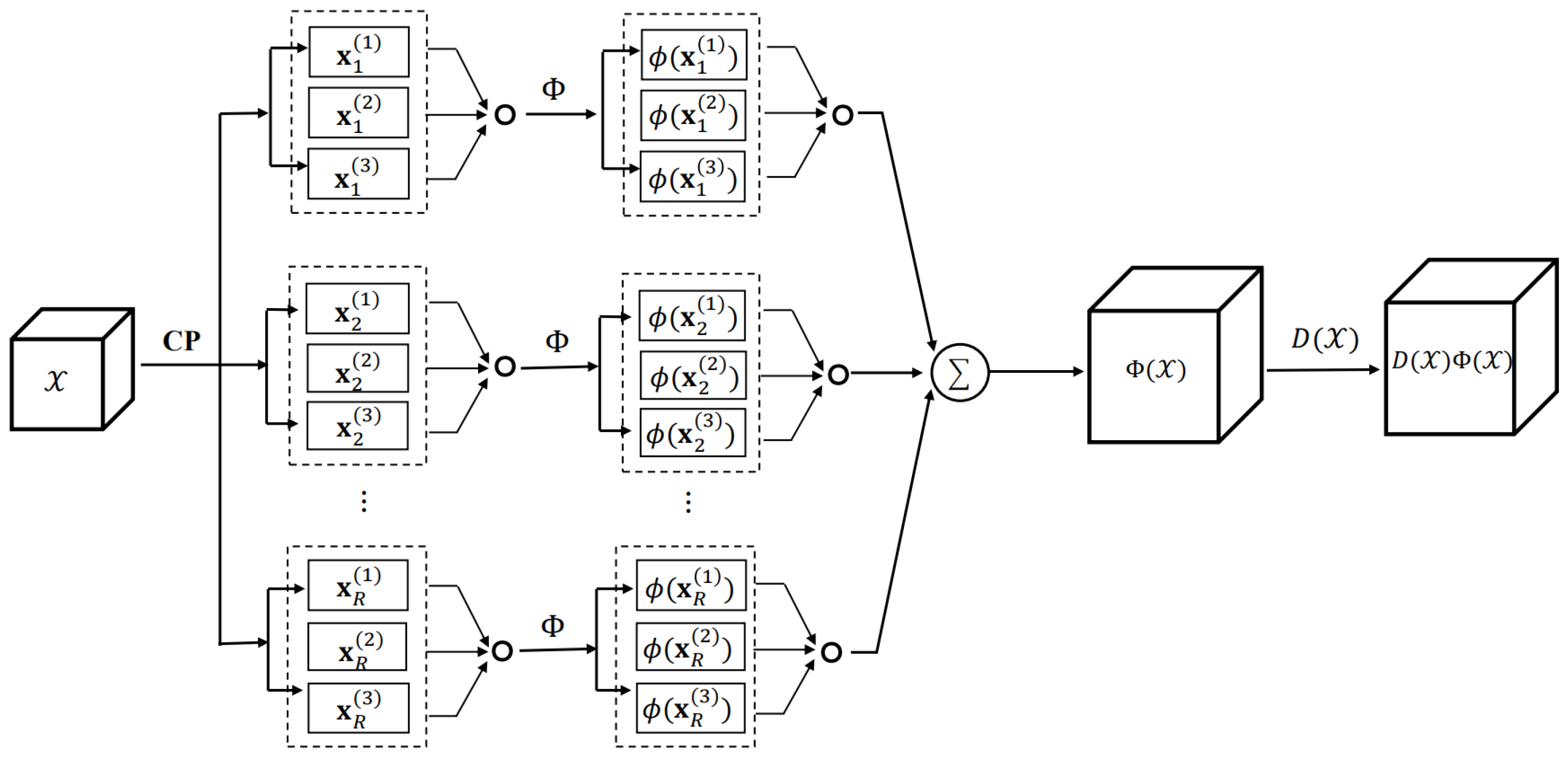
where $D\left(\mathcal{X}\right):=exp(-\mu f{\left(\mathcal{X}\right)}^2)$ with a tunable parameter $\mu >0$. The visualization of the kernel scaling in the learning process is shown in Figure 3, where the flowchart of scaling nonlinear mapping is represented in Figure 4.

For any rank-one tensor $\mathcal{X}={\prod }_{n=1}^N\circ {\mathbf{x}}^{\left(n\right)}$,

$$\begin{array}{c}\hfill D\left(\mathcal{X}\right)=exp\left\{-\mu {\left[\sum _{i\in T^{*}}{\alpha }_i{y}_{i}exp\left\{\frac{{\displaystyle \sum _{n=1}^N}{\parallel {\mathbf{x}}^{\left(n\right)}-{\mathbf{x}}_i^{\left(n\right)}\parallel }^2}{-2{\sigma }^2}\right\}+b\right]}^2\right\}=:\Theta ({\mathbf{x}}^{\left(1\right)},\cdots ,{\mathbf{x}}^{\left(N\right)}).\end{array}$$

Let $\tilde{\mathcal{Z}}=D\left(\mathcal{X}\right)\Phi \left(\mathcal{X}\right)=\Theta ({\mathbf{x}}^{\left(1\right)},\cdots ,{\mathbf{x}}^{\left(N\right)})\Phi \left(\mathcal{X}\right)$. We have the following property.

Lemma 2.

$\parallel d\tilde{\mathcal{Z}}{\parallel }_F^2=D{\left(\mathcal{X}\right)}^2\left({\left[d\left(log\Theta ({\mathbf{x}}^{\left(1\right)},\cdots ,{\mathbf{x}}^{\left(N\right)})\right)\right]}^2+{\parallel d\mathcal{Z}\parallel }_F^2\right)$.

Proof. 

By the definitions of $D\left(\mathcal{X}\right)$ and $\tilde{\mathcal{Z}}$, we have

$$d\tilde{\mathcal{Z}}=d(\Theta ({\mathbf{x}}^{\left(1\right)},\cdots ,{\mathbf{x}}^{\left(N\right)}))\Phi \left(\mathcal{X}\right)+\Theta ({\mathbf{x}}^{\left(1\right)},\cdots ,{\mathbf{x}}^{\left(N\right)})d(\Phi \left(\mathcal{X}\right))$$

and $d(\Theta ({\mathbf{x}}^{\left(1\right)},\cdots ,{\mathbf{x}}^{\left(N\right)}))=D\left(\mathcal{X}\right)d\left(log\Theta ({\mathbf{x}}^{\left(1\right)},\cdots ,{\mathbf{x}}^{\left(N\right)})\right)$. Additionally, invoking expressions in (9) and (10), we have

$$〈\Phi \left(\mathcal{X}\right),\Phi \left(\mathcal{X}\right)〉=1\mathrm{and}〈\Phi \left(\mathcal{X}\right),d(\Phi (\mathcal{X}\left)\right)〉=0.$$

(12)

Thus,

$$\begin{array}{c}\hfill \begin{array}{cc}\parallel d\tilde{\mathcal{Z}}{\parallel }_F^2\hfill & =\parallel d(\Theta ({\mathbf{x}}^{\left(1\right)},\cdots ,{\mathbf{x}}^{\left(N\right)}))\Phi \left(\mathcal{X}\right)+\Theta ({\mathbf{x}}^{\left(1\right)},\cdots ,{\mathbf{x}}^{\left(N\right)})d(\Phi \left(\mathcal{X}\right)){\parallel }_F^2\hfill \\ & ={\left(d(\Theta ({\mathbf{x}}^{\left(1\right)},\cdots ,{\mathbf{x}}^{\left(N\right)}))\right)}^2\langle \Phi \left(\mathcal{X}\right),\Phi \left(\mathcal{X}\right)\rangle +D{\left(\mathcal{X}\right)}^2\langle d(\Phi \left(\mathcal{X}\right)),d(\Phi \left(\mathcal{X}\right))\rangle \hfill \\ & +2D\left(\mathcal{X}\right)d(\Theta ({\mathbf{x}}^{\left(1\right)},\cdots ,{\mathbf{x}}^{\left(N\right)}))\langle \Phi \left(\mathcal{X}\right),d(\Phi \left(\mathcal{X}\right))\rangle \hfill \\ & ={\left(d(\Theta ({\mathbf{x}}^{\left(1\right)},\cdots ,{\mathbf{x}}^{\left(N\right)}))\right)}^2+D{\left(\mathcal{X}\right)}^2{\parallel d\left(\mathcal{Z}\right)\parallel }_F^2\hfill \\ & =D{\left(\mathcal{X}\right)}^2\left({\left[d\left(log\Theta ({\mathbf{x}}^{\left(1\right)},\cdots ,{\mathbf{x}}^{\left(N\right)})\right)\right]}^2+{\parallel d\mathcal{Z}\parallel }_F^2\right)\hfill \end{array}\end{array}$$

where the third equality follows from (12). This completes the proof.    □

Obviously, $\parallel d\tilde{\mathcal{Z}}{\parallel }_F^2={\parallel d\mathcal{Z}\parallel }_F^2$ for any $\mathcal{X}$ on the boundary $f\left(\mathcal{X}\right)=0$. Notice that

$$\begin{array}{c}\hfill d\left(log\Theta ({\mathbf{x}}^{\left(1\right)},\cdots ,{\mathbf{x}}^{\left(N\right)})\right)=D^{\left[1\right]\top }d{\mathbf{x}}^{\left(1\right)}+\cdots +D^{\left[N\right]\top }d{\mathbf{x}}^{\left(N\right)},\end{array}$$

where $D^{\left[n\right]}=\frac{\partial log\Theta ({\mathbf{x}}^{\left(1\right)},\cdots ,{\mathbf{x}}^{\left(N\right)})}{\partial {\mathbf{x}}^{\left(n\right)}}$. Denote $Q_{i,j}=\langle D^{\left[i\right]},D^{\left[j\right]}\rangle$, it follows that

$$\begin{array}{c}\hfill \begin{array}{cc}& \parallel d\left(log\Theta ({\mathbf{x}}^{\left(1\right)},\cdots ,{\mathbf{x}}^{\left(N\right)})\right){\parallel }^2\hfill \\ =\hfill & \left[d{\mathbf{x}}^{\left(1\right)\top },\cdots ,d{\mathbf{x}}^{\left(N\right)\top }\right]\left[\begin{array}{ccc}{Q}_{1,1}& \cdots & Q_{1,N}\\ Q_{2,1}& \cdots & Q_{2,N}\\ ⋮& \cdots & ⋮\\ Q_{N-1,1}& \cdots & Q_{N-1,N}\\ Q_{N,1}& \cdots & Q_{N,N}\end{array}\right]\left[\begin{array}{c}d{\mathbf{x}}^{\left(1\right)}\\ ⋮\\ d{\mathbf{x}}^{\left(N\right)}\end{array}\right].\hfill \end{array}\end{array}$$

(13)

Now, focusing on a neighborhood of support tensors ${\mathcal{X}}_i$, there is

$$\begin{array}{c}\hfill \Theta ({\mathbf{x}}^{\left(1\right)},\cdots ,{\mathbf{x}}^{\left(N\right)})=exp\left\{-\mu {\left[{\alpha }_i{y}_{i}exp\left\{\frac{{\displaystyle \sum _{n=1}^N}{\parallel {\mathbf{x}}^{\left(n\right)}-{\mathbf{x}}_i^{\left(n\right)}\parallel }^2}{-2{\sigma }^2}\right\}+b\right]}^2\right\}.\end{array}$$

For convenience, we denote $\parallel d\tilde{\mathcal{Z}}{\parallel }_F^2={\displaystyle \sum _{i=1}^{\Xi }}{\displaystyle \sum _{j=1}^{\Xi }}\tilde{G}{\left(\mathcal{X}\right)}_{ij}d{v}_{i}d{v}_j$, $\tilde{\rho }\left(\mathcal{X}\right)=\sqrt{det\left(\tilde{G}\left(\mathcal{X}\right)\right)}$. Then we can state the following theorem:

Theorem 1.

The ratio of the magnification factors $\tilde{\rho }\left(\mathcal{X}\right)$ and $\rho \left(\mathcal{X}\right)$ is

$$\begin{array}{c}\hfill \frac{\tilde{\rho }\left(\mathcal{X}\right)}{\rho \left(\mathcal{X}\right)}=D{\left(\mathcal{X}\right)}^{\Xi }\sqrt{1+{\sigma }^2{\parallel \nabla log\Theta ({\mathbf{x}}^{\left(1\right)},\cdots ,{\mathbf{x}}^{\left(N\right)})\parallel }_F^2}.\end{array}$$

(14)

Proof. 

According to Lemma 2 and (13), we have

$$\begin{array}{c}\hfill \begin{array}{cc}\parallel d\tilde{\mathcal{Z}}{\parallel }_F^2\hfill & =D{\left(\mathcal{X}\right)}^2\left({\left[d\left(log\Theta ({\mathbf{x}}^{\left(1\right)},\cdots ,{\mathbf{x}}^{\left(N\right)})\right)\right]}^2+{\parallel d\mathcal{Z}\parallel }_F^2\right)\hfill \\ & ={\displaystyle \sum _{i=1}^{\Xi }}{\displaystyle \sum _{j=1}^{\Xi }}\tilde{G}{\left(\mathcal{X}\right)}_{ij}d{v}_{i}d{v}_j,\hfill \end{array}\end{array}$$

where

$$\begin{array}{c}\hfill \begin{array}{c}\tilde{G}\left(\mathcal{X}\right)=D{\left(\mathcal{X}\right)}^2\left[\begin{array}{ccc}{Q}_{1,1}& \cdots & Q_{1,N}\\ Q_{2,1}& \cdots & Q_{2,N}\\ ⋮& \cdots & ⋮\\ Q_{N,1}& \cdots & Q_{N,N}\end{array}\right]+D{\left(\mathcal{X}\right)}^{2}G\left(\mathcal{X}\right).\hfill \end{array}\end{array}$$

Since $\tilde{\rho }\left(\mathcal{X}\right)=\sqrt{det(\tilde{G}\left(\mathcal{X}\right))}$, there is

$$\frac{\tilde{\rho }\left(\mathcal{X}\right)}{\rho \left(\mathcal{X}\right)}=D{\left(\mathcal{X}\right)}^{\Xi }\sqrt{1+{\sigma }^2{\parallel \nabla \log \Theta ({\mathbf{x}}^{\left(1\right)},\cdots ,{\mathbf{x}}^{\left(N\right)})\parallel }_F^2}.$$

This completes the proof.    □

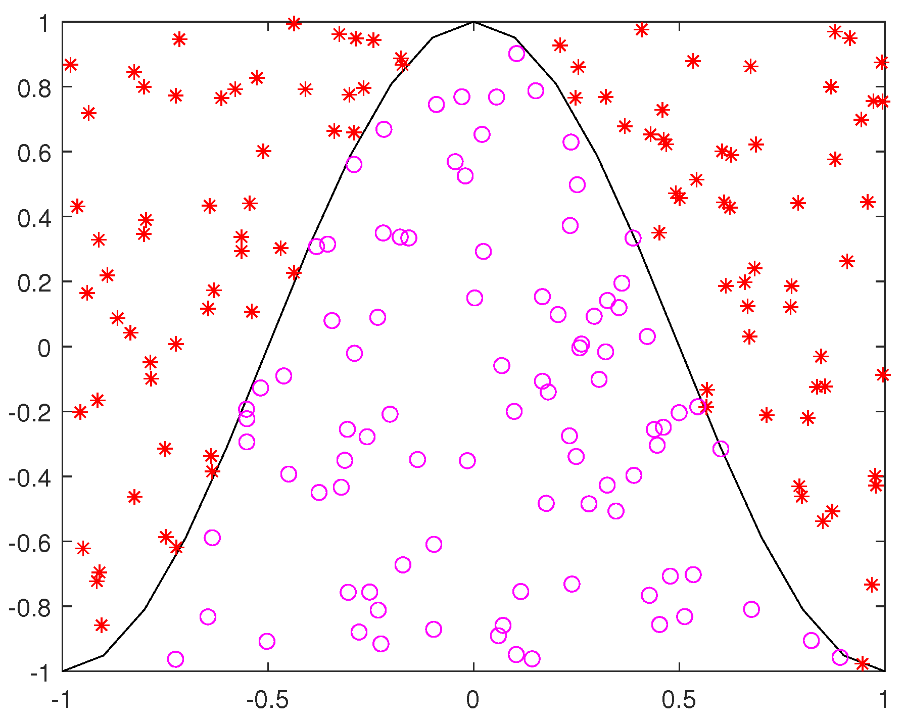
To visualize the performance of the scaling strategy, we follow the approach by [32] to randomly generate $\left\{{\mathbf{x}}^{\left(i\right)}={\left(x_1^{\left(i\right)},x_2^{\left(i\right)}\right)}^{\top }:i=1,\dots ,200\right\}$, which follows the i.i.d. uniform distribution in the region $[-1,1]\times [-1,1]$ and can be separated by $x_2=cos\left(\pi x_1\right)$; see Figure 5. The symbols with different type and color represent different categories.

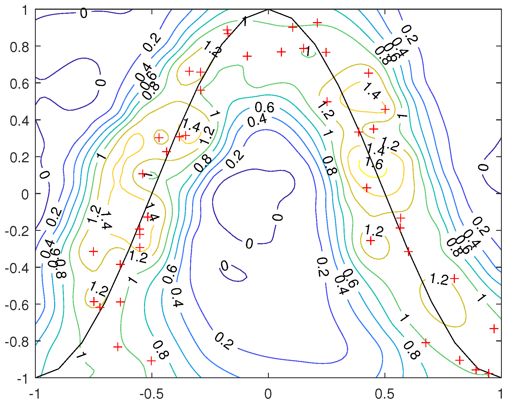
By applying ‘LIBSVM’ with 80% of samples for training and 20% for testing, we test the performance with fixed values of $C=2^2,\sigma =0.50$, and $\mu =0.20$. The classification accuracy is $90.00$% in the first stage and $97.50$% in the second stage with the scaled scheme. To visualize the effect of the scaling strategy, we plot the contours of the ratio magnification factors as defined in (14) in Figure 6, along with SVs marked by ‘+’, distributing around the boundary $f\left(x\right)=0$. One can easily find that the magnification factor in the neighborhood that covers these SVs is greater than 1, indicating an enlargement in the magnification factor at these SVs. In contrast, the magnification factors in non-SVs are reduced after scaling. The enlargement-reduction scenario will facilitate the detection of the classification boundary, leading to a reasonable improvement in classification accuracy.

4.3. The Proposed NKSTM Approach

To effectively solve the non-convex and discontinuous problem, i.e., Problem (7), the Newton-type method, denoted as NSSVM, proposed by Zhou [35], is employed. The gradient and the Hessian of the objective function in Problem (7) are

$$\nabla \mathrm{Y}\left(\mathbf{\alpha }\right):=H\left(\mathbf{\alpha }\right)\mathbf{\alpha }-\mathbf{1},H\left(\mathbf{\alpha }\right):=\mathbb{K}+E\left(\mathbf{\alpha }\right).$$

Since $\mathbb{K}$ is the Hadamard product of two symmetric positive semidefinite matrices and, hence, positive semidefinite, and $E\left(\mathbf{\alpha }\right)$ is a diagonal positive definite matrix, we can see that $H\left(\mathbf{\alpha }\right)$ is positive definite. For notational convenience, we denote $\mathbf{z}:={({\mathbf{\alpha }}^{\top },b)}^{\top }\in {\mathbb{R}}^{M+1}$, and

$$\begin{array}{c}\hfill \begin{array}{ccc}h\left(\mathbf{z}\right)\hfill & :=\hfill & \nabla \mathrm{Y}\left(\mathbf{\alpha }\right)+\mathbf{y}b=H\left(\mathbf{\alpha }\right)\mathbf{\alpha }-\mathbf{1}+\mathbf{y}b,\hfill \\ h_T\left(\mathbf{z}\right)\hfill & :=\hfill & {\left(h\left(\mathbf{z}\right)\right)}_T,\hfill \\ H_T\left(\mathbf{\alpha }\right)\hfill & :=\hfill & {\left(H\left(\mathbf{\alpha }\right)\right)}_{TT},\hfill \end{array}\end{array}$$

where $T:=\mathrm{supp}\left(\mathbf{\alpha }\right)$ is the support set, $h_T\left(\mathbf{\alpha }\right)$ is a sub-vector of the vector $h\left(\mathbf{z}\right)$ indexed by T, $H_T\left(\mathbf{\alpha }\right)$ is the sub-principal matrix of the matrix $H\left(\mathbf{\alpha }\right)$ with rows and columns both indexed by T. We denote $\overline{T}:=\left[M\right]\setminus T$, and

$$\begin{array}{c}\hfill {\mathbb{T}}_s\left(\mathbf{\alpha }\right):=\left\{T\subseteq \left[M\right]:\begin{array}{c}\left|T\right|=s,\hfill \\ |{\mathbf{\alpha }}_i|\ge |{\mathbf{\alpha }}_j|,\forall i\in T,\forall j\in \overline{T}\hfill \end{array}\right\},\end{array}$$

where $\left|T\right|$ is the cardinality of T, which counts the number of elements in T. Following from [35], we also introduce the stationary equation system for Problem (7) in the form of

$$\begin{array}{c}\hfill F(\mathbf{z};T):=\left[\begin{array}{c}{h}_T\left(\mathbf{z}\right)\\ {\mathbf{\alpha }}_{\overline{T}}\\ \langle {\mathbf{\alpha }}_T,{\mathbf{y}}_T\rangle \end{array}\right]=\mathbf{0}.\end{array}$$

After choosing the index set $T_k\in {\mathbb{T}}_s({\mathbf{\alpha }}^k-\eta h\left({\mathbf{z}}^k\right))$, the Newton direction ${\mathbf{d}}^k\in {\mathbb{R}}^{M+1}$ can be found by solving the linear equations $\nabla F({\mathbf{z}}^k;T_k){\mathbf{d}}^k=-F({\mathbf{z}}^k;T_k)$. Then, the algorithmic framework for solving sparse STM can be summarized as follows.

Equipped with the kernel scaling scheme, the framework of the resulting two-stage training process with NSSVM can be described as in Algorithm 1.

Algorithm 1 (re-NKSTM) NKSTM with the rescaling kernel.

Input: Training dataset ${\{{\mathcal{X}}_i,y_i\}}_{i=1}^M$, parameters $C>c,\eta ,ϵ,K,\mu >0,s\in \left[M\right]$, the CP rank R.

Output: The solution ${\tilde{\mathbf{z}}}^k$.

Step 1: Initialize ${\mathbf{z}}^0$, pick $T_0\in {\mathbb{T}}_s({\mathbf{\alpha }}^0-\eta h\left({\mathbf{z}}^0\right))$, and $k:=0$;

Step 2: Compute ${\mathbf{z}}^{k+1}$ by NSSVM with the tensorial RBF kernel $\kappa (·,·)$;

Step 3: If the stopping criterion is satisfied, then go to Step 4; otherwise, set $k=k+1$ and go to Step 2;

Step 4: Compute the modified kernel $\tilde{\kappa }(·,·)$ by (11) to rescale the primal kernel $\kappa (·,·)$;

Step 5: Compute ${\tilde{\mathbf{z}}}^{k+1}$ by NSSVM with the tensorial RBF kernel $\tilde{\kappa }(·,·)$;

Step 6: If the stopping criterion is satisfied, then stop; otherwise, set $k=k+1$ and go to Step 5.

Convergence and complexity analysis. Note that Algorithm 2 is indeed the first stage in Algorithm 1. It follows from Theorem 3.1 in [35] that Algorithm 2 enjoys the one-step convergence if the initial point is chosen to be close to a local region of a stationary point. The computational complexity in each iteration of Algorithm 2 is analyzed as follows:

• The main term involved in computing $H_{T_k}\left({\mathbf{\alpha }}^k\right)={\mathbb{K}}_{T_k{T}_k}+E{\left(\mathbf{\alpha }\right)}_{T_k{T}_k}$ is ${\mathbb{K}}_{T_k{T}_k}$, which has a complexity of about $O\left(s^2{R}^2{\displaystyle \sum _{n=1}^N}{I}_n\right)$ since $|T_k|=s$, and computing the inverse of $H_{T_k}\left({\mathbf{\alpha }}^k\right)$ requires at most $O\left(s^3\right)$;
• To pick $T_{k+1}\in {\mathbb{T}}_s({\mathbf{\alpha }}^k-\eta h\left({\mathbf{z}}^k\right))$, we need to compute $h\left({\mathbf{z}}^k\right)$ and pick out the k largest elements of $|{\mathbf{\alpha }}^k-\eta h\left({\mathbf{z}}^k\right)|$. The complexity of computing the former is $O\left(M^2\right)$ and the latter is $O(M+s\ln s)$.

Algorithm 2 (NKSTM) Newton-kernelized STM.

Input: Training dataset ${\{{\mathcal{X}}_i,y_i\}}_{i=1}^M$, the parameters $C>c,\eta ,ϵ,K>0,s\in \left[M\right]$, the CP rank R.

Output: The solution ${\mathbf{z}}^k$.

Step 1: Initialize ${\mathbf{z}}^0$, pick $T_0\in {\mathbb{T}}_s({\mathbf{\alpha }}^0-\eta h\left({\mathbf{z}}^0\right))$, and $k:=0$;

Step 2: Compute ${\mathbf{z}}^{k+1}$ by NSSVM with the tensorial RBF kernel;

Step 3: If the stopping criterion is satisfied, then stop; otherwise, set $k=k+1$ and go to Step 2.

Overall, the whole computational complexity in each iteration of both Algorithms 1 and 2 is of the following order:

$$O\left(s^{2}max\left\{R^2\sum _{n=1}^N{I}_n,s\right\}+M^2\right).$$

Note that the computations of tensorial RBF kernels in both Algorithms 1 and 2 heavily rely on the CP decompositions of tensor samples ${\left\{{\mathcal{X}}_i\right\}}_{i=1}^M$, which are performed by using the ALS algorithm with line search [42]. Since these CP decompositions are performed just once in Algorithms 1 and 2, we omit the complexity analysis here. The storage complexity is $O\left(M{\displaystyle \sum _{n=1}^N}{I}_n+s^2\right)$.

5. Numerical Experiments

We conducted numerical experiments on real datasets to evaluate the efficiency of the proposed sparse STM approach. All the computational results were obtained using a laptop running on a 64-bit Windows Operating System with an (Intel(R) Core(TM) i7-8565U CPU @1.8 GHz RAM 8.0 G), equipped with Matlab R2018b with the Tensor Toolbox Version 3.1, (https://gitlab.com/tensors/tensortoolbox, accessed on 1 June 2019).

Normalization is applied to each of the raw sample tensors, denoted as $\{{\tilde{\mathcal{X}}}_j:j\in \left[M\right]\}$, for more efficient data processing. Specifically, for each $j\in \left[M\right]$, the normalized tensor ${\mathcal{X}}_j$ is generated by

$${\left({\mathcal{X}}_j\right)}_{i_1{i}_2\cdots i_N}=\frac{{\left({\tilde{\mathcal{X}}}_j\right)}_{i_1{i}_2\cdots i_N}-{\tilde{\mathcal{X}}}_j^{min}}{{\tilde{\mathcal{X}}}_j^{max}-{\tilde{\mathcal{X}}}_j^{min}},\forall i_1,i_2,\dots ,i_N,$$

with ${\tilde{\mathcal{X}}}_j^{min}$ and ${\tilde{\mathcal{X}}}_j^{max}$ being the minimal and the maximal entries of ${\tilde{\mathcal{X}}}_j$, respectively.

Experimental setup. To construct the tensor kernels among $\{{\mathcal{X}}_j:j\in \left[M\right]\}$, we use the grid search on $\{1,\cdots ,8\}$ to choose the CP rank R and adopt the ALS algorithm with line search in [42] to obtain the low-rank CP decomposition approximations. For the RBF kernel parameter $\sigma$ and hyperparameter C, we adopt grid search to pick them from $\{2^{-3},\cdots ,2^5\}$, and $\{2^0,2^1,\cdots ,2^9\}$, respectively, and set $c=0.01C$. For simplicity, the scaling parameter $\mu$ in the second stage is chosen as $\frac{1}{I_1{I}_2\cdots I_N}$ and adaptively changed in high-dimensionality problems. The sparsity level parameter s is chosen based on the testing instances.

For NKSTM, we choose the initialization point ${\mathbf{z}}^{\mathbf{0}}={({\mathbf{\alpha }}_0^{\top },b)}^{\top }$ with ${\mathbf{\alpha }}^0=\mathbf{0}$ and $b^0=\mathrm{sgn}\left(\langle \mathbf{y},1\rangle \right)$, and set the stationarity parameter $\eta =min(\frac{1}{M},{10}^{-4})$ from [35]. The algorithm will be terminated if one of the following criteria is satisfied: (i) reaching the maximum iteration number $K=1000$; (ii) meeting the halting conditions:

$$\begin{array}{c}\hfill \begin{array}{c}\parallel F({\mathbf{z}}^k;T_k)\parallel <ϵ,|\mathrm{acc}\left({\mathbf{\alpha }}^k\right)-\underset{j\in [k-1]}{max}\mathrm{acc}\left({\mathbf{\alpha }}^j\right)|<{10}^{-4},\end{array}\end{array}$$

where $ϵ=\sqrt{M{I}_1\cdots I_N}\times {10}^{-6}$, $\mathrm{acc}\left(\mathbf{\alpha }\right)$ is the training accuracy defined by

$$\mathrm{acc}\left(\mathbf{\alpha }\right)=\left[1-\frac{1}{M}\parallel \mathrm{sgn}\left(\mathbf{K}(\mathbf{\alpha }\odot \mathbf{y})+b\mathbf{1}\right)-\mathbf{y}{\parallel }_0\right]\times 100\%,$$

(15)

with acc$\left({\mathbf{\alpha }}^{-1}\right)=0$ by default. The testing classification accuracy is defined in the same way as in (15) by replacing the training samples with the testing samples.

5.1. Benchmark Methods

We compare the classification accuracy of the proposed approach with the accuracy of the following existing methods.

• LIBSVM: SVM with hinge loss was implemented by Lin et al. [47], which is one of the most popular classification methods based on vector space. In this paper, we consider the SVM with a Gaussian kernel.
• NSSVM-RBF: NSSVM based on vector space was developed by Zhou [35] for data reduction, which is a linearly kernelized SVM optimization problem with sparsity constraints. We consider the Gaussian RBF kernel for nonlinearly separable data.
• DuSK: He et al. [24] proposed a dual structure-preserving kernel based on CP decomposition for supervised tensor learning to boost tensor classification performances. In the experiment, we chose the Gaussian RBF kernel.
• TT-MMK: Kour et al. [27] introduced a tensor train multi-way multi-level kernel (TT-MMK), which converts the available TT decomposition into the CP decomposition for kernelized classification. The Gaussian RBF kernel was adopted in the article.

For fair comparisons, the default settings of all other competitor approaches will be adopted, and the rank selections in all rank-related methods will be determined in the same way as in our proposed methods. All numerical results show the average performance with five-fold cross-validation in 5 trials for all tested methods. For convenience, we simply use ‘TRACC1’ (‘TEACC1’) and ‘TRACC2’ (‘TEACC2’) to refer to the training (testing) accuracies of the NKSTM and re-NKSTM approaches, respectively.

5.2. StarPlus fMRI Dataset

We conduct the numerical experiments using the magnetic resonance imaging (fMRI) images in the field of neuroscience. Each is represented in a third-order tensor format, as illustrated in Figure 7 from [24]. We choose images from the StarPlus dataset www.cs.cmu.edu/afs/cs.cmu.edu/project/theo-81/www, accessed on 1 June 2019, which are in the form of a tensor with dimensions of $64\times 64\times 8$, containing 25 to 30 anatomically defined regions (denoted as “Regions of Interest", or ROIs). In order to improve the classification accuracy, the following ROIs are taken into consideration: ‘CALC’, ‘LIPL’, ‘LT’, ‘LTRIA’, ‘LOPER’, ‘LIPS’, and ‘LDLPFC’. More details about data preprocessing are explained in [26]. Here, we pick subject 04799 from [26] to test the classification performance. This subject contains 320 fMRI images: half of them were collected when the subject was shown a picture, and the other half were collected when the subject was shown a sentence. In the five-fold CV, 256 samples are used for training and 64 for testing in each classification trial.

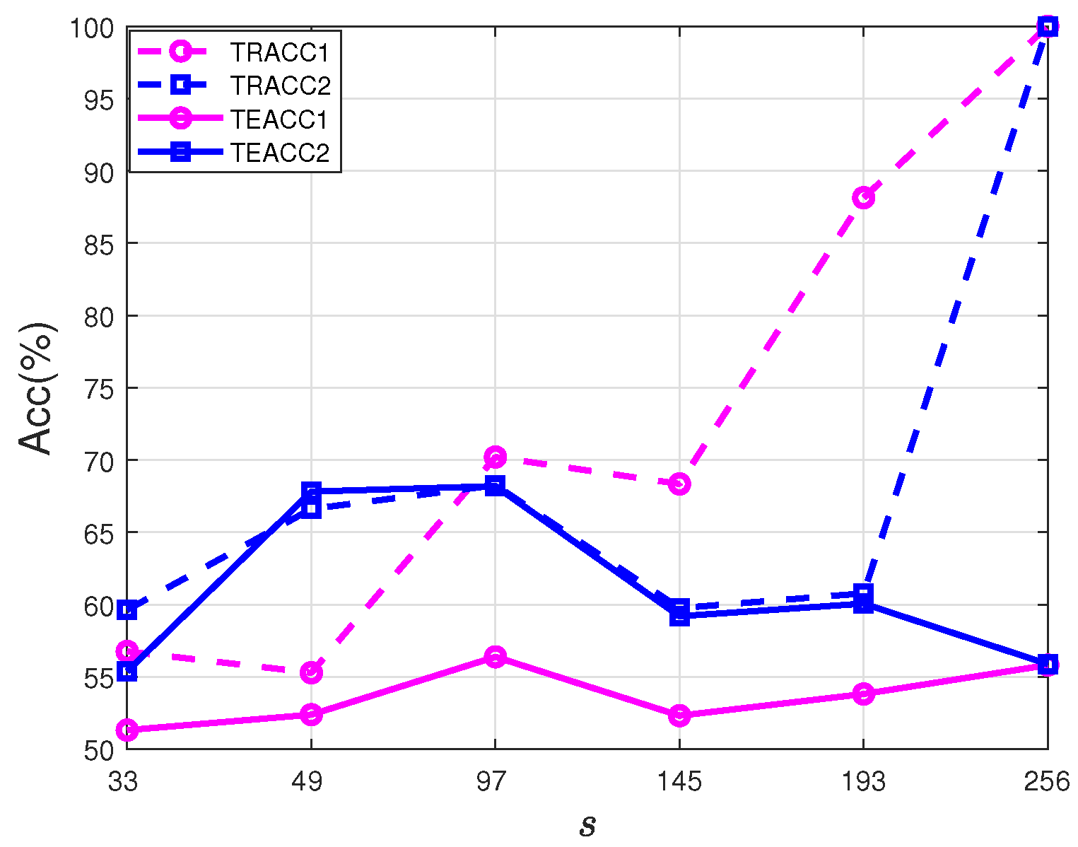
To test the effect of the sparsity level s in the proposed model (7), we simply choose the CP rank $R=2$, and record the training and the testing accuracies with different values of $s\in \{33,49,97,145,193,256\}$ in Figure 8. It is not surprising to see in Figure 8 that the re-NKSTM in the second stage shows better performance than NKSTM in the testing accuracy, and achieves its peak testing accuracy in a sparse setting with $s=97$ among the instances. As shown in this figure, the effect of the sparsity constraint imposed on $\mathbf{\alpha }$ is positive, with a reasonable sacrifice on the training accuracy to alleviate the overfitting.

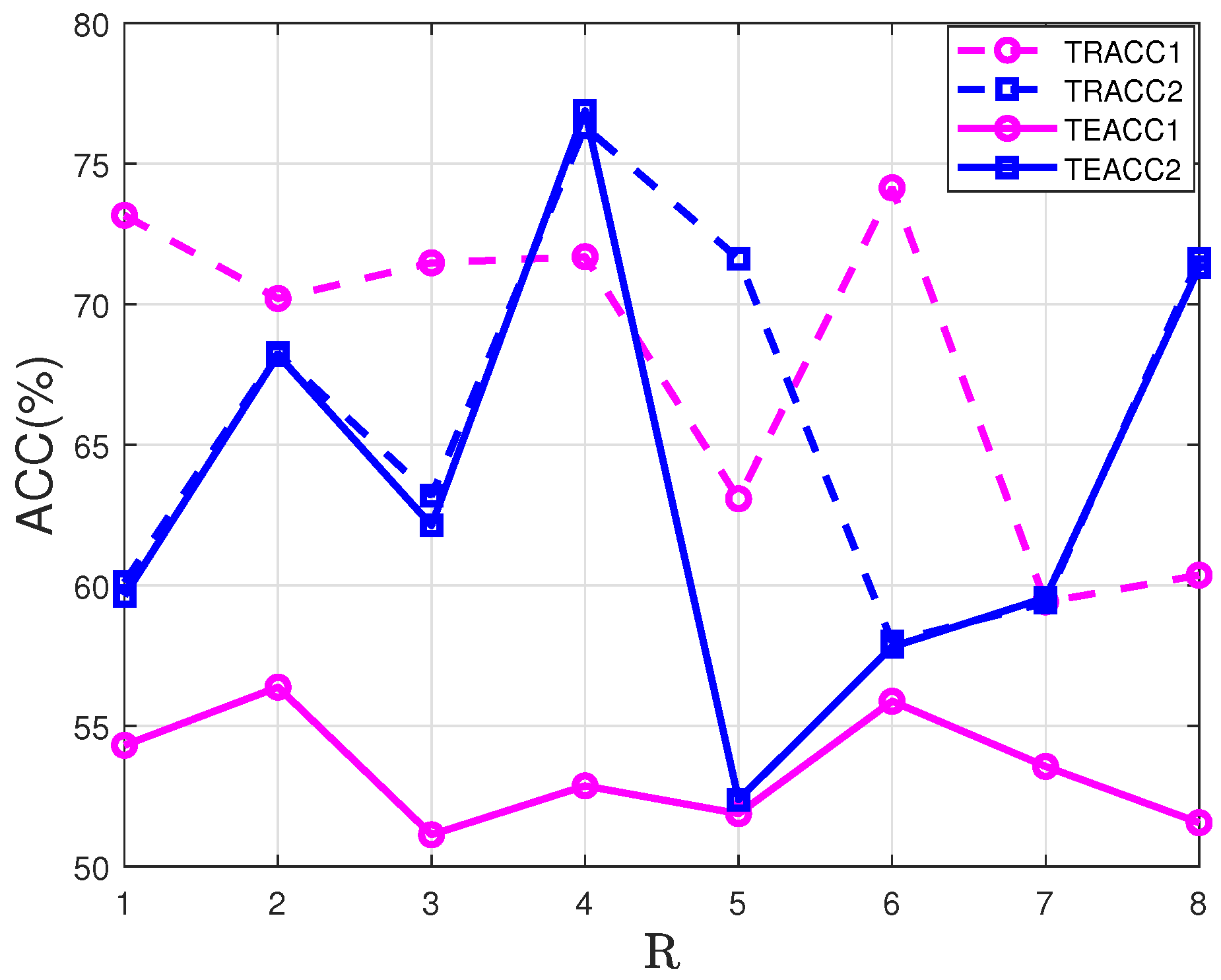
To test the effect of the CP rank R, we choose $s=97$, as discussed above, and collect the training and testing accuracies with different values of $R\in \{1,2,3,\dots ,8\}$ in Figure 9. The superiority of re-NKSTM in the testing accuracy is confirmed again in these instances. In particular, in the case of CP rank $R=4$, the accuracy in the second stage is 76.88%, which is 24% higher than 52.87% in the first stage. Moreover, the choice of CP rank $R=4$ for re-NKSTM shows the best performance in both training and testing, which, to some extent, indicates the advantage of imposing the low-rankness assumption on tensor samples for classification.

Table 2. The classification accuracy (%) comparison for subject ‘04799’.

re-NKSTM	NKSTM	LIBSVM	NSSVM-RBF	DuSK	TT-MMK
76.88	52.87	50.00	50.00	56.37	57.44

The best result is highlighted in bold.

presents the classification accuracies between the proposed approach and several state-of-the-art methods. Here, in the NKSTM and re-NKSTM approaches, we choose $s=97$, and in all rank-related methods (NKSTM, re-NKSTM, DuSK, TT-MMK), the grid search is used to choose the corresponding tensor rank. As can be seen in Table 2, the testing accuracy of re-NKSTM is about 20% higher than those of other competitors. In particular, the scaled kernel scheme in re-NKSTM achieves a classification accuracy that is 24% higher than that of NKSTM without any scaled kernel function.

5.3. CIFAR-10 Dataset

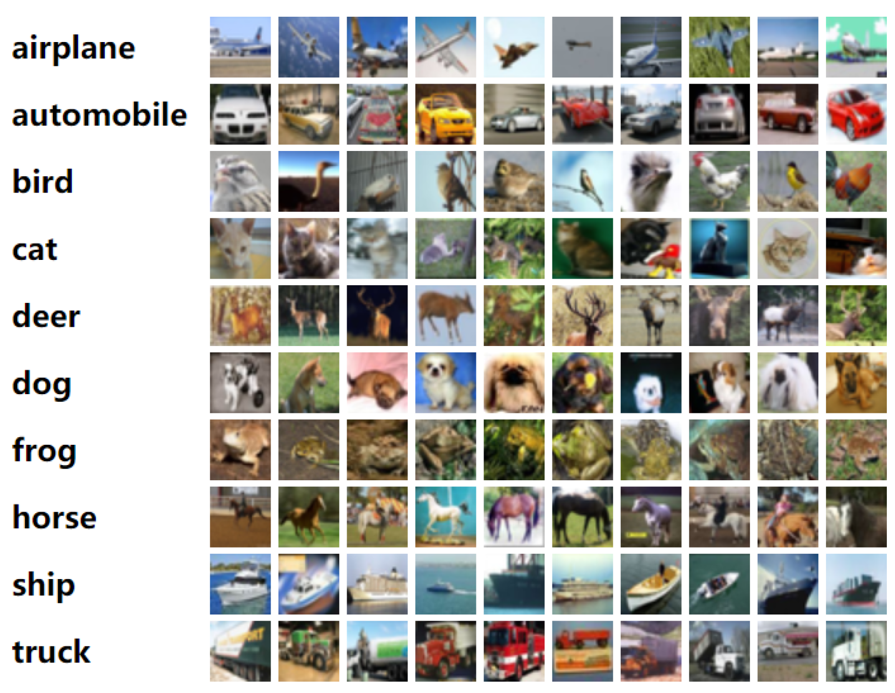
Each color picture from the CIFAR-10 [48] dataset, as shown in Figure 10, can be deemed as a third-order tensor (pixel–pixel–color) with dimensions of $32\times 32\times 3$. We randomly select nine class pairs to perform the binary classification. Without overlap, we choose 100 samples from the dataset in each class to obtain 200 samples for each class pair classification (160 for training and 40 for testing).

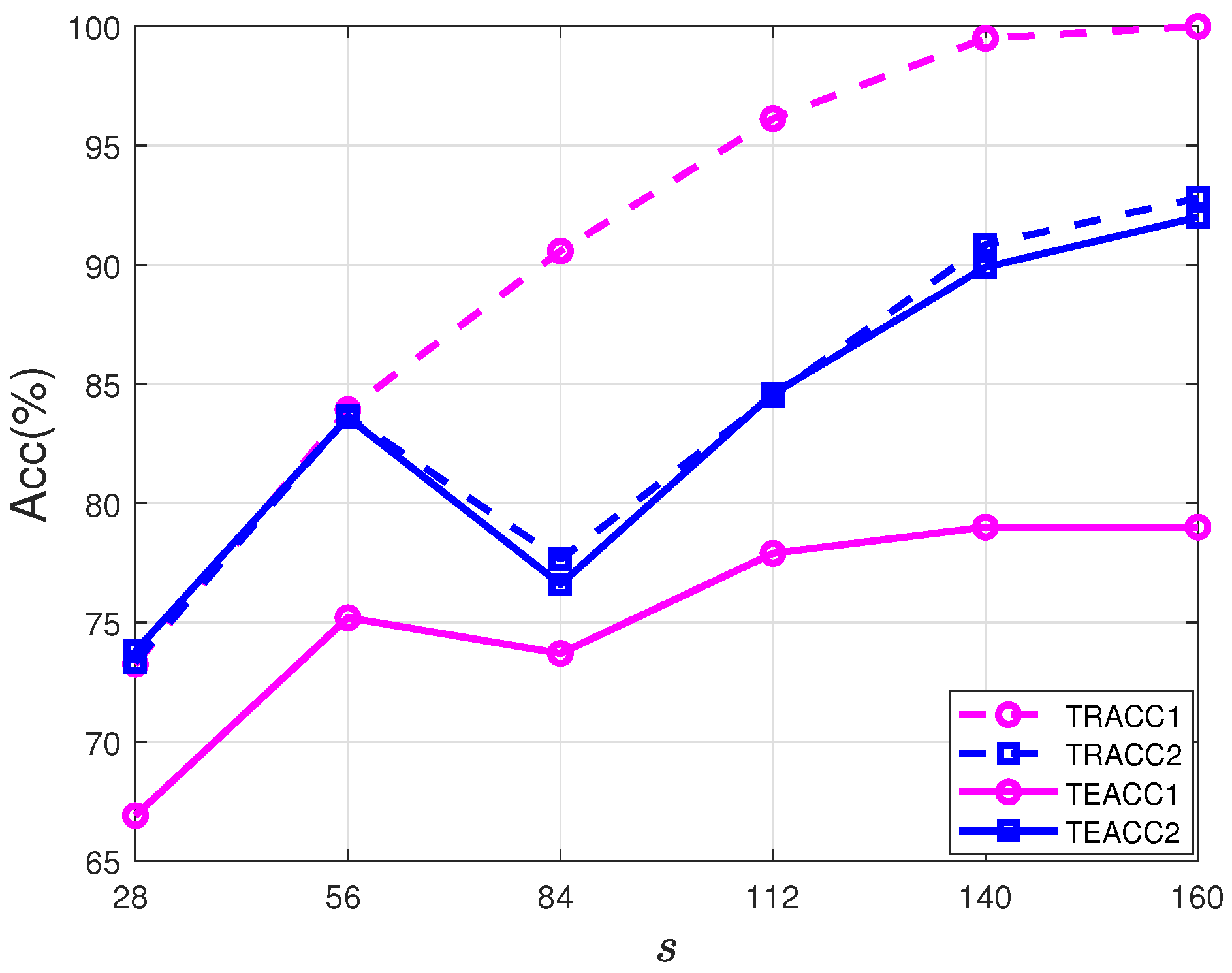
Similarly, we test the effect of the sparsity level in the proposed NKSTM and re-NKSTM approaches. The class pair ‘automobile-cat’ is chosen for illustration. The training and the testing accuracies of these two approaches with different values of $s\in \{28,56,84,112,140,160\}$ are shown in Figure 11, by fixing the CP rank $R=1$. One can observe that re-NKSTM outperforms NKSTM in the testing accuracy for all tested instances; for the sparse setting $s=112$, both the training and testing accuracies approach a high percentage of 85%.

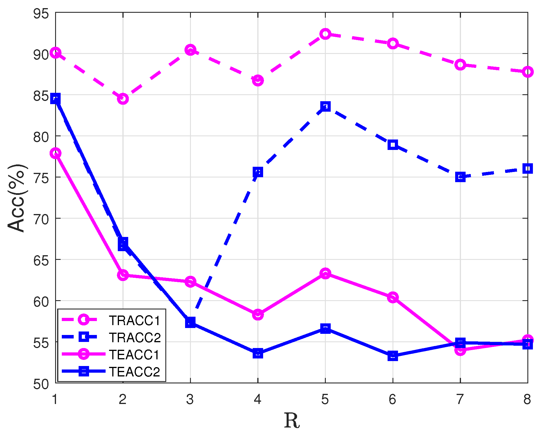
We also test the effect of the CP rank in the proposed NKSTM and re-NKSTM approaches by fixing $s=112$. The results with the CP rank R varying among $\{1,2,3,\dots ,8\}$ are reported in Figure 12. As can be seen in this figure, the NKSTM and re-NKSTM approaches gain the best classification performances at $R=1$, with accuracies of about $78\%$ for NKSTM and $85\%$ for re-NKSTM.

Table 3. The classification accuracy (%) comparison for the CIFAR-10 dataset.

Class Pair	re-NKSTM	NKSTM	LIBSVM	NSSVM-RBF	DuSK	TT-MMK
‘bird, deer’	75.40	67.50	62.50	60.70	73.00	73.40
‘deer, horse’	88.30	66.10	54.70	71.10	70.30	71.20
‘bird, horse’	90.00	69.40	71.10	72.90	73.20	76.10
‘truck, ship’	82.90	75.30	76.40	75.80	78.40	78.20
‘automobile, ship’	83.30	74.40	60.30	77.70	78.30	77.30
‘automobile, cat’	84.60	77.90	65.80	77.10	79.10	79.50
‘automobile, horse’	79.20	75.00	72.50	78.60	76.40	75.90
‘air, ship’	73.10	65.90	65.10	69.80	68.70	71.50
‘automobile, truck’	87.10	69.00	58.10	71.90	73.10	72.20

The best result is highlighted in bold.

lists the comparison results for nine class pairs by performing the aforementioned six algorithms. Here, we set $s=112$ in the NKSTM and re-NKSTM approaches, and use the experiment setup as described at the beginning of this section for all algorithms. As one can see from Table 3, re-NKSTM outperforms all other five approaches in classification accuracy for all tested instances, and the superiority is mainly achieved in the scaled kernel scheme when compared with the results of NKSTM. In particular, for the ‘bird & horse’ classification, the accuracy is 90.00% in re-NKSTM, which improved by about 20% compared to 69.40% for NKSTM.

6. Conclusions

In this paper, a sparse STM model based on the dual structure-preserving kernel function was proposed for the binary classification of tensorial data. Scaling kernel functions were embedded to alleviate the local risks caused by the constant Gaussian RBF kernel width in the presence of uneven spatial distributions, and a two-stage approach equipped with the subspace Newton method was designed in the learning process. Numerical experiments conducted on real datasets have confirmed the superiority of the proposed approach in classification accuracy.

However, there are still limitations to the proposed method. For example, the time efficiency of the tensor decomposition in the kernel function evaluation process needs to be improved, especially for high-dimensional and high-order tensor samples. Moreover, the effectiveness of the proposed approach was demonstrated numerically in terms of the classification accuracy, and the analysis of the generalization ability needs to be further studied from a theoretical perspective. In addition, as the 0/1 loss was recognized as the ideal loss function to characterize the number of misclassified samples, the kernelized sparse STM with such a loss will be a promising model, which deserves further study in future research.

References

1. Liu, J.; Zhu, C.; Long, Z.; Liu, Y. Tensor regression. Found. Trends Mach. Learn. 2021, 14, 379–565. [Google Scholar] [CrossRef]
2. Kolda, T.; Bader, B. Tensor decompositions and applications. SIAM Rev. 2009, 51, 455–500. [Google Scholar] [CrossRef]
3. Xing, Y.; Wang, M.; Yang, S.; Zhang, K. Pansharpening with multiscale geometric support tensor machine. IEEE Geosci. Remote Sens. Lett. 2018, 56, 2503–2517. [Google Scholar] [CrossRef]
4. Zhang, L.; Zhang, L.; Tao, D.; Huang, X. A multifeature tensor for remote-sensing target recognition. IEEE Geosci. Remote Sens. Lett. 2011, 8, 374–378. [Google Scholar] [CrossRef]
5. Zhou, B.; Song, B.; Hassan, M.; Alamri, A. Multilinear rank support tensor machine for crowd density estimation. Eng. Appl. Artif. Intel. 2018, 72, 382–392. [Google Scholar] [CrossRef]
6. Zhao, Z.; Chow, T. Maximum margin multisurface support tensor machines with application to image classification and segmentation. Expert Syst. Appl. 2012, 39, 849–860. [Google Scholar]
7. He, Z.; Shao, H.; Cheng, J.; Zhao, X.; Yang, Y. Support tensor machine with dynamic penalty factors and its application to the fault diagnosis of rotating machinery with unbalanced data. Mech. Syst. Signal Process. 2020, 141, 106441. [Google Scholar] [CrossRef]
8. Hu, C.; He, S.; Wang, Y. A classification method to detect faults in a rotating machinery based on kernelled support tensor machine and multilinear principal component analysis. Appl. Intell. 2021, 51, 2609–2621. [Google Scholar] [CrossRef]
9. Tao, D.; Li, X.; Hu, W.; Maybank, S.; Wu, X. Supervised tensor learning. In Proceedings of the Fifth IEEE International Conference on Data Mining, Houston, TX, USA, 27–30 November 2005; pp. 450–457. [Google Scholar]
10. Tao, D.; Li, X.; Wu, X.; Hu, W.; Maybank, S. Supervised tensor learning. Knowl. Inf. Syst. 2007, 13, 1–42. [Google Scholar] [CrossRef]
11. Kotsia, I.; Patras, I. Support tucker machines. In Proceedings of the IEEE Conference on Computer Vision and Pattern Recognition (CVPR), IEEE, Colorado Springs, CO, USA, 20–25 June 2011; pp. 633–640. [Google Scholar]
12. Khemchandani, R.; Karpatne, A.; Chandra, S. Proximal support tensor machines. Int. J. Mach. Learn. Cyber. 2013, 4, 703–712. [Google Scholar] [CrossRef]
13. Chen, C.; Batselier, K.; Ko, C.Y.; Wong, N. A support tensor train machine. In Proceedings of the 2019 International Joint Conference on Neural Networks, Budapest, Hungary, 14–19 July 2019; pp. 1–8. [Google Scholar]
14. Sun, T.; Sun, X. New results on classification modeling of noisy tensor datasets: A fuzzy support tensor machine dual model. IEEE Trans. Syst. Man Cybern. 2021, 99, 1–13. [Google Scholar] [CrossRef]
15. Chen, Y.; Wang, K.; Zhong, P. One-class support tensor machine. Knowl.-Based Syst. 2016, 96, 14–28. [Google Scholar] [CrossRef] [Green Version]
16. Zhang, X.; Gao, X.; Wang, Y. Twin support tensor machines for MC detection. J. Electron. 2009, 26, 318–325. [Google Scholar] [CrossRef]
17. Shi, H.; Zhao, X.; Zhen, L.; Jing, L. Twin bounded support tensor machine for classification. Int. J. Pattern Recogn. 2016, 30, 1650002.1–1650002.20. [Google Scholar] [CrossRef]
18. Rastogi, R.; Sharma, S. Ternary tree based-structural twin support tensor machine for clustering. Pattern Anal. Appl. 2021, 24, 61–74. [Google Scholar] [CrossRef]
19. Yan, S.; Xu, D.; Yang, Q.; Zhang, L.; Tang, X.; Zhang, H. Multilinear discriminant analysis for face recognition. IEEE Trans. Image Process. 2007, 16, 212–220. [Google Scholar] [CrossRef] [PubMed]
20. Lu, H.; Plataniotis, K.; Venetsanopoulos, A. MPCA: Multilinear principal component analysis of tensor objects. IEEE Trans. Neural Netw. 2008, 19, 18–39. [Google Scholar] [PubMed] [Green Version]
21. Kotsia, I.; Guo, W.; Patras, I. Higher rank support tensor machines for visual recognition. Pattern Recognit. 2012, 45, 4192–4203. [Google Scholar] [CrossRef]
22. Yang, B. Research and Application of Machine Learning Algorithm Based Tensor Representation; China Agricultural University: Beijing, China, 2017. [Google Scholar]
23. Rubinov, M.; Knock, S.; Stam, C.; Micheloyannis, S.; Harris, A.; Williams, L.; Breakspear, M. Small-world properties of nonlinear brain activity in schizophrenia. Hum. Brain Mapp. 2009, 30, 403–416. [Google Scholar] [CrossRef] [PubMed]
24. He, L.; Kong, X.; Yu, P.; Ragin, A.; Hao, Z.; Yang, X. DuSK: A dual structure-preserving kernel for supervised tensor learning with applications to neuroimages. In Proceedings of the 2014 SIAM International Conference on Data Mining SIAM, Philadelphia, PA, USA, 24–26 April 2014; pp. 127–135. [Google Scholar]
25. He, L.; Lu, C.; Ma, G.; Wang, S.; Shen, L.; Yu, P.; Ragin, A. Kernelized support tensor machines. In Proceedings of the 34th International Conference on Machine Learning, Sydney, Australia, 6–11 August 2017; Volume 70, pp. 1442–1451. [Google Scholar]
26. Chen, C.; Batselier, K.; Yu, W.; Wong, N. Kernelized support tensor train machines. Pattern Recognit. 2022, 122, 108337. [Google Scholar] [CrossRef]
27. Kour, K.; Dolgov, S.; Stoll, M.; Benner, P. Efficient structure-preserving support tensor train machine. J. Mach. Learn. Res. 2023, 24, 1–22. [Google Scholar]
28. Deng, X.; Shi, Y.; Yao, D.; Tang, X.; Mi, C.; Xiao, J.; Zhang, X. A kernelized support tensor-ring machine for high-dimensional data classification. In Proceedings of the International Conference on Electronic Information Technology and Smart Agriculture (ICEITSA), IEEE, Huaihua, China, 10–12 December 2021; pp. 159–165. [Google Scholar]
29. Scholkopf, B.; Burges, C.; Smola, A. Advances in Kernel Methods; MIT Press: Cambridge, MA, USA, 1999. [Google Scholar]
30. Amari, S.; Wu, S. Improving support vector machine classifiers by modifying kernel functions. Neural Netw. 1999, 12, 783–789. [Google Scholar] [CrossRef] [PubMed]
31. Wu, S.; Amari, S. Conformal transformation of kernel functions: A data-dependent way to improve support vector machine classifiers. Neural Process. Lett. 2001, 25, 59–67. [Google Scholar]
32. Williams, P.; Li, S.; Feng, J.; Wu, S. Scaling the kernel function to improve performance of the support vector machine. In International Symposium on Neural Networks; Springer: Berlin/Heidelberg, Germany, 2005; pp. 831–836. [Google Scholar]
33. Williams, P.; Wu, S.; Feng, J. Improving the performance of the support vector machine: Two geometrical scaling methods. StudFuzz 2005, 177, 205–218. [Google Scholar]
34. Chang, Q.; Chen, Q.; Wang, X. Scaling Gaussian RBF kernel width to improve SVM classification. In Proceedings of the International Conference on Neural Networks and Brain, Beijing, China, 13–15 October 2005. [Google Scholar]
35. Zhou, S. Sparse SVM for sufficient data reduction. IEEE Trans. Pattern Anal. Mach. Intell. 2022, 44, 5560–5571. [Google Scholar] [CrossRef]
36. Wang, S.; Luo, Z. Low rank support tensor machine based on L0/1 soft-margin loss function. Oper. Res. Trans. 2021, 25, 160–172. (In Chinese) [Google Scholar]
37. Lian, H. Learning rate for convex support tensor machines. IEEE Trans. Neural Netw. Learn. Syst. 2021, 32, 3755–3760. [Google Scholar] [CrossRef]
38. Shu, T.; Yang, Z.X. Support tensor machine based on nuclear norm of tensor. J. Neijiang Norm. Univ. 2017, 32, 34–39. (In Chinese) [Google Scholar]
39. He, L.F.; Lu, C.T.; Ding, H.; Wang, S.; Shen, L.L.; Yu, P.; Ragin, A.B. Multi-way multi-level kernel modeling for neuroimaging classification. In Proceedings of the IEEE Conference on Computer Vision and Pattern Recognition, Honolulu, HI, USA, 21–26 July 2017; pp. 356–364. [Google Scholar]
40. Hao, Z.; He, L.; Chen, B.; Yang, X. A linear support higher-order tensor machine for classification. IEEE Trans. Image Process. 2013, 22, 2911–2920. [Google Scholar] [PubMed]
41. Qi, L.; Luo, Z. Tensor Analysis: Spectral Theory and Special Tensors; SIAM Press: Philadelphia, PA, USA, 2017. [Google Scholar]
42. Nion, D.; Lathauwer, L. An enhanced line search scheme for complex-valued tensor decompositions. Application in DS-CDMA. Signal Process. 2008, 21, 749–755. [Google Scholar] [CrossRef]
43. Steinwart, I.; Christmann, A. Support Vector Machines; Springer: New York, NY, USA, 2008. [Google Scholar]
44. Zhao, L.; Mammadov, M.J.; Yearwood, J. From convex to nonconvex: A loss function analysis for binary classification. In Proceedings of the IEEE International Conference on Data Mining Workshops, Sydney, NSW, Australia, 13 December 2010; pp. 1281–1288. [Google Scholar]
45. Wang, Q.; Ma, Y.; Zhao, K.; Tian, Y. A comprehensive survey of loss functions in machine learning. Ann. Data. Sci. 2022, 9, 187–212. [Google Scholar] [CrossRef]
46. Wang, H.; Xiu, N. Analysis of loss functions in support vector machines. Adv. Math. 2021, 50, 801–828. (In Chinese) [Google Scholar]
47. Chang, C.; Lin, C. LIBSVM: A library for support vector machines. ACM Trans. Intel. Syst. Tec. 2011, 2, 1–27. [Google Scholar] [CrossRef]
48. Krizhevsky, A.; Hinton, G. Learning Multiple Layers of Features from Tiny Images; Technical Report; University of Toronto: Toronto, ON, Canada, 2009. [Google Scholar]
Figure 1. A flowchart of the proposed approach for binary classification.
Mathematics 11 02829 g001
Figure 2. CP decomposition of a third-order tensor.
Mathematics 11 02829 g002
Figure 3. A flowchart of the scaling kernel function.
Mathematics 11 02829 g003
Figure 4. Scaling nonlinear mapping with the CP decomposition.
Mathematics 11 02829 g004
Figure 5. The binary classification for 200 randomly generated points.
Mathematics 11 02829 g005
Figure 6. The contours of the ratio of magnification factors (14) for training data.
Mathematics 11 02829 g006
Figure 7. fMRI images: (a) The third-order tensor format; (b) the visualization.
Mathematics 11 02829 g007
Figure 8. Effect of the sparsity level s with R = 2 .
Mathematics 11 02829 g008
Figure 9. Effect of the CP rank with s = 97 .
Mathematics 11 02829 g009
Figure 10. CIFAR-10 dataset.
Mathematics 11 02829 g010
Figure 11. Effect of s with R = 1 .
Mathematics 11 02829 g011
Figure 12. Effect of CP rank with s = 112 .
Mathematics 11 02829 g012