Abstract
In this paper, we detail closed form estimators for beta distribution that are simpler than those proposed by Tamae, Irie and Kubokawa. The proposed estimators are shown to have smaller asymptotic variances and smaller asymptotic covariances compared to Tamae estimators and maximum likelihood estimators. The proposed estimators are also shown to perform better in real data applications.
MSC:
62E99
1. Introduction
The most popular model for data in a finite interval is that based on the beta distribution. It is a two parameter distribution with probability density function given by
for , and , where denotes the beta function defined by
which can be equivalently expressed as , where denotes the gamma function. We shall write to mean that a random variable X has the beta distribution. The mean and variance of are
respectively. There are hundreds if not thousands of papers on the theory and applications of the beta distribution. It is impossible to cite all of these papers. Comprehensive accounts of the theory and applications of the beta distribution can be found in [1,2,3,4,5]. See also [6].
For a long time, estimating parameters of the beta distribution and other related distributions, such as the gamma distribution, was only possible through iteration methods. For instance, if x is an observation on then maximum likelihood estimators of and , say and , respectively, can be obtained by solving
where , and denotes the digamma function. Furthermore, the corresponding asymptotic variances and asymptotic covariance are given by
as , where denotes the trigamma function, , , and . Furthermore, let .
However, recently closed form estimators for the gamma and beta distributions have been proposed. Ref. [7] proposed closed form estimators for the gamma distribution by considering the likelihood equations of the generalized gamma distribution and taking the gamma distribution as a special case. Ref. [8] proposed closed form estimators for the gamma and beta distributions using the “score adjusted approach”. The estimators for the gamma distribution in [8] turned out to be the same as those obtained by [7].
Following the method applied by [8], two closed form and simpler estimators for the beta distribution are proposed in this paper. The two estimators appear to have smaller variances and smaller covariances for certain values of the parameters of the beta distribution.
The remainder of this paper is organized as follows. Section 2 re-derives the closed form estimators for the beta distribution due to [8]. Section 3 derives two new closed form estimators for the beta distribution. Section 4 establishes asymptotic normality of the new estimators. It also derives expressions for asymptotic variances and asymptotic covariances. Section 5 conducts a numerical comparison to show that the new estimators can be better than the estimators due to [8] as well as maximum likelihood estimators. A simulation study is conducted in Section 6 to check finite sample performance of all the estimators. Section 7 shows that the new estimators can provide better fit to a real dataset. Finally, some conclusions are given in Section 8. All computations in the paper were performed using the R software [9]. Sample code are given in Appendix A.
2. Tamae et al.’s [8] Closed Form Estimators
Let . Using the facts
and
we can show that
and
Subtracting (5) from (4), using (1), (2) and (3) and solving for gives
which implies
Another way of expressing (6) is
Substituting from (6) into (7) and solving for yields
By the weak law of large numbers, we can replace the expectations in (6) and (8) by their sample versions yielding the closed form estimators proposed by [8] as
The corresponding asymptotic variances and asymptotic covariance are given by
as .
3. New Closed Form Estimators
In this section, we propose two new estimators for and . Throughout, we suppose that .
Substituting (3) into (5) and rearranging the terms gives
which implies
Multiplying (9) by , using (1) and solving for gives
Substituting (10) in (9) and solving for gives
By the weak law of large numbers, we can replace the expectations in (10) and (11) by sample versions to obtain the estimators:
Substituting (1) and (2) in (4) and rearranging yields
which implies
Multiplying (13) by , using (1) and solving for gives
Substituting (14) in (13) and solving for gives
By the weak law of large numbers, we can replace the expectations in (14) and (15) by their sample versions to obtain
Note that . This relationship can be useful in deriving large sample properties given in Section 4.
4. Large Sample Properties
Large sample properties of the estimators given by (12) and (16) are derived in this section. Theorem 1 proves asymptotic normality of the estimators given by (12). Theorem 2 proves asymptotic normality of the estimators given by (16).
Theorem 1.
The estimators given in (12) satisfy
as , where
and
Proof.
Let the empirical means of X, , and be denoted by , , and , respectively. We can easily show that
and
We can also show that
Using the fact that
we can show that
Similarly, we can show that
and
By the central limit theorem,
as , where
and
The entries of this matrix are given by (1) and (17)–(21) as
and
Let , and . Then
and
Let
Using the delta method,
as , where
and
where
and
The theorem follows by simplification of these expressions. □
Proof.
Let the empirical means of X, and be denoted by , and , respectively. We can easily show that
and
We can also show that
Using the fact that
we have
Similarly, we can show that
and
By the central limit theorem,
as , where
The entries of this matrix are given by (1) and (22)–(26) as
and
Let , and . Then,
and
Let
Using the delta method,
as , where
where
and
The theorem follows by simplification of these expressions. □
5. Numerical Comparison
In this section, we compare the asymptotic variances and asymptotic covariances of the estimators given by Theorems 1 and 2, Tamae et al.’s estimators and maximum likelihood estimators. Figure 1, Figure 2 and Figure 3 show how the asymptotic variances and asymptotic covariances of these estimators vary versus and . Figure 4, Figure 5 and Figure 6 show the differences in asymptotic variances and the differences in asymptotic covariances for two of the estimators at a time as and . We shall refer to Tamae et al.’s estimators as TIK estimators.
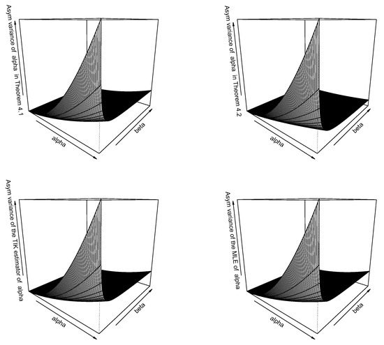
Figure 1.
Asymptotic variance of the estimator of versus and for the estimator given by Theorem 1 (top left), the estimator given by Theorem 2 (top right), TIK estimator (bottom left), and maximum likelihood estimator (bottom right).
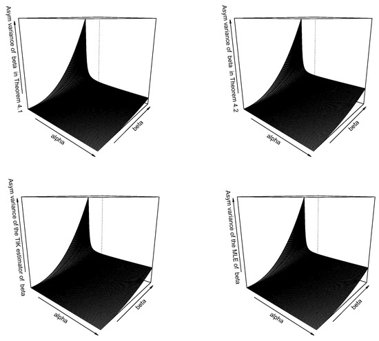
Figure 2.
Asymptotic variance of the estimator of versus and for the estimator given by Theorem 1 (top left), the estimator given by Theorem 2 (top right), TIK estimator (bottom left), and maximum likelihood estimator (bottom right).
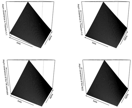
Figure 3.
Asymptotic covariance between the estimators of and versus and for the estimators given by Theorem 1 (top left), the estimators given by Theorem 2 (top right), TIK estimators (bottom left), and maximum likelihood estimators (bottom right).
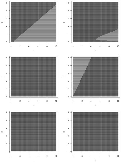
Figure 4.
Sign of the difference between the asymptotic variances of the estimators of given by Theorems 1 and 2 (top left); sign of the difference between the asymptotic variances of the estimator of given by Theorem 1 and TIK estimator (top right); sign of the difference between the asymptotic variances of the estimator of given by Theorem 1 and maximum likelihood estimator (middle left); sign of the difference between the asymptotic variances of the estimator of given by Theorem 2 and TIK estimator (middle right); sign of the difference between the asymptotic variances of the estimator of given by Theorem 2 and maximum likelihood estimator (bottom left); sign of the difference between the asymptotic variances of TIK estimator of and maximum likelihood estimator (bottom right).
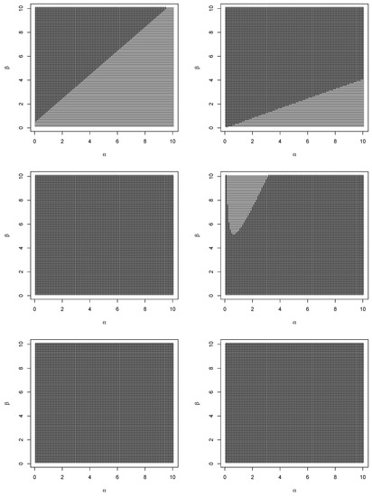
Figure 5.
Sign of the difference between the asymptotic variances of the estimators of given by Theorems 1 and 2 (top left); sign of the difference between the asymptotic variances of the estimator of given by Theorem 1 and TIK estimator (top right); sign of the difference between the asymptotic variances of the estimator of given by Theorem 1 and maximum likelihood estimator (middle left); sign of the difference between the asymptotic variances of the estimator of given by Theorem 2 and TIK estimator (middle right); sign of the difference between the asymptotic variances of the estimator of given by Theorem 2 and maximum likelihood estimator (bottom left); sign of the difference between the asymptotic variances of TIK estimator of and maximum likelihood estimator (bottom right).
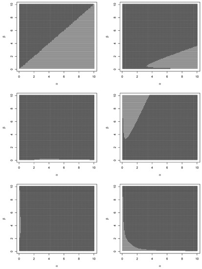
Figure 6.
Sign of the difference between the asymptotic covariances of the estimators given by Theorems 1 and 2 (top left); sign of the difference between the asymptotic covariances of the estimators given by Theorem 1 and TIK estimator (top right); sign of the difference between the asymptotic covariances of the estimators given by Theorem 1 and maximum likelihood estimator (middle left); sign of the difference between the asymptotic covariances of the estimators given by Theorem 2 and TIK estimator (middle right); sign of the difference between the asymptotic covariances of the estimators given by Theorem 2 and maximum likelihood estimator (bottom left); sign of the difference between the asymptotic covariances of TIK estimator and maximum likelihood estimator (bottom right).
We can observe the following from Figure 1, Figure 2 and Figure 3. Asymptotic variances of all of the estimators for increase with respect to ; asymptotic variances of all of the estimators for decrease with respect to ; asymptotic variances of all of the estimators for decrease with respect to ; asymptotic variances of all of the estimators for increase with respect to ; asymptotic covariances of all of the estimators increase with respect to ; and asymptotic covariances of all of the estimators increase with respect to . All four estimators in each of the Figure 1, Figure 2 and Figure 3 appear to behave similarly.
We can observe the following from Figure 4, Figure 5 and Figure 6. With respect to asymptotic variances of the estimators for , the estimator in Theorem 1 is more efficient than the corresponding estimator in Theorem 2 for all ; with respect to asymptotic variances of the estimators for , the estimator in Theorem 1 is more efficient than the corresponding TIK estimator in a parabolic region containing large values of and small values of ; with respect to asymptotic variances of the estimators for , the maximum likelihood estimator is more efficient than the corresponding estimator in Theorem 1 for all values of and ; with respect to asymptotic variances of the estimators for , the estimator in Theorem 2 is more efficient than the corresponding TIK estimator for all ; with respect to asymptotic variances of the estimators for , the maximum likelihood estimator is more efficient than the corresponding estimator in Theorem 2 and the corresponding TIK estimator for all values of and ; with respect to asymptotic variances of the estimators for , the estimator in Theorem 1 is more efficient than the corresponding estimator in Theorem 2 for all ; with respect to asymptotic variances of the estimators for , the estimator in Theorem 1 is more efficient than the corresponding TIK estimator for all ; with respect to asymptotic variances of the estimators for , the estimator in Theorem 2 is more efficient than the corresponding TIK estimator in a parabolic region containing small values of and large values of ; with respect to asymptotic variances of the estimators for , the maximum likelihood estimator is more efficient than the three remaining estimators for all values of and ; with respect to asymptotic covariances, the estimators in Theorem 1 are more efficient than the corresponding estimators in Theorem 2 for all ; with respect to asymptotic covariances, the estimators in Theorem 1 are more efficient than the corresponding TIK estimators in a parabolic region containing large values of and small values of ; with respect to asymptotic covariances, the estimators in Theorem 1 are more efficient than the corresponding maximum likelihood estimators for all small values of ; with respect to asymptotic covariances, the estimators in Theorem 2 are more efficient than the corresponding TIK estimators in a parabolic region containing small values of and large values of ; with respect to asymptotic covariances, the estimators in Theorem 2 are more efficient than the corresponding maximum likelihood estimators for all small values of ; and with respect to asymptotic covariances, the TIK estimators are more efficient than the corresponding maximum likelihood estimators in a hyperbolic region containing either small values of both and or small values of and large values of or large values of and small values of .
In summary, we can see that the estimators in Theorem 1 can be more efficient than the TIK estimators if either or in a parabolic region containing large values of and small values of . The estimators in Theorem 1 can be more efficient than the maximum likelihood estimators for small values of . The estimators in Theorem 2 can be more efficient than the TIK estimators if either or in a parabolic region containing large values of and small values of . The estimators in Theorem 2 can be more efficient than the maximum likelihood estimators for small values of . The estimators in Theorem 1 can be more efficient than the estimators in Theorem 2 if .
6. Simulation Study
Finite sample performances of the estimators given by Theorems 1 and 2, Tamae et al.’s estimators and maximum likelihood estimators are compared in this section. We use the following simulation scheme:
- (i)
- Simulate a random sample of size n from a beta distribution with parameters and ;
- (ii)
- Compute the estimators given by Theorems 1 and 2, Tamae et al.’s estimators and maximum likelihood estimators;
- (iii)
- Repeat steps (i) and (ii) 1000 times;
- (iv)
- Compute the bias and mean squared error of the estimators;
- (v)
- Compute also the p-value for [10]’s test of bivariate normality of the estimators;
- (vi)
- Repeat steps (i) to (v) for .
Biases versus n for all four estimators are shown in Figure 7. Mean squared errors versus n for all four estimators are shown in Figure 8. p-values versus n for all four estimators are shown in Figure 9.
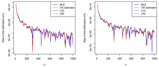
Figure 7.
Biases of the estimators of a (left) and b (right) versus n.
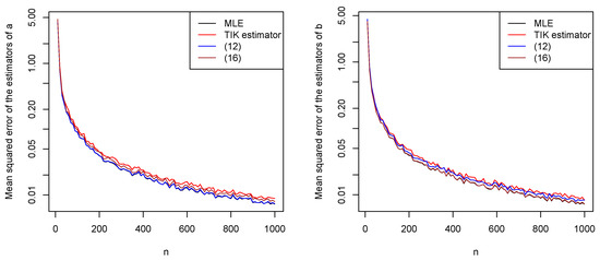
Figure 8.
Mean squared errors of the estimators of a (left) and b (right) versus n.
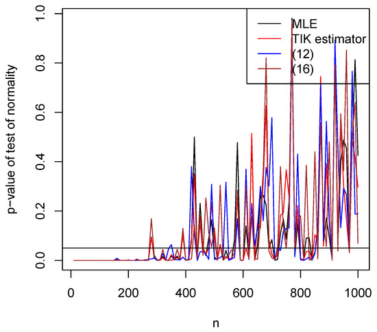
Figure 9.
P-values for [10]’s test of bivariate normality of the estimators versus n. The horizontal line corresponds to 0.05.
We observe the following from the figures: increasing n leads the biases generally decreasing to zero; the relative performances of the estimators with respect to bias appear similar; the biases appear reasonably small for all ; increasing n leads the mean squared errors generally decreasing to zero; the mean squared errors appear largest for Tamae et al.’s estimators and smallest for maximum likelihood estimators; the mean squared errors appear reasonably small for all ; asymptotic normality of all estimators appears to have been achieved for all .
These observations are for and . However, the same observations held for a wide range of other values of a and b. In particular, increasing n always led to the biases decreasing to zero, increasing n always led to the mean squared errors decreasing to zero, and the mean squared errors always appeared largest for Tamae et al.’s estimators and smallest for maximum likelihood estimators.
7. Real Data Illustration
In this section, we compare the performance of the estimators given by Theorems 1 and 2, Tamae et al.’s estimators and maximum likelihood estimators using a real dataset. The data are the proportion voting Remain in the Brexit (EU referendum) poll outcomes for 127 polls from January 2016 to the referendum date on June 2016. The actual data values are 0.52, 0.55, 0.51, 0.49, 0.44, 0.54, 0.48, 0.41, 0.45, 0.42, 0.53, 0.45, 0.44, 0.44, 0.42, 0.42, 0.37, 0.46, 0.43, 0.39, 0.45, 0.44, 0.46, 0.40, 0.48, 0.42, 0.44, 0.45, 0.43, 0.43, 0.48, 0.41, 0.43, 0.40, 0.41, 0.42, 0.44, 0.51, 0.44, 0.44, 0.41, 0.41, 0.45, 0.55, 0.44, 0.44, 0.52, 0.55, 0.47, 0.43, 0.55, 0.38, 0.36, 0.38, 0.44, 0.42, 0.44, 0.43, 0.42, 0.49, 0.39, 0.41, 0.45, 0.43, 0.44, 0.51, 0.51, 0.49, 0.48, 0.43, 0.53, 0.38, 0.40, 0.39, 0.35, 0.45, 0.42, 0.40, 0.39, 0.44, 0.51, 0.39, 0.35, 0.41, 0.51, 0.45, 0.49, 0.40, 0.48, 0.41, 0.46, 0.47, 0.43, 0.45, 0.48, 0.49, 0.40, 0.40, 0.40, 0.39, 0.41, 0.39, 0.48, 0.48, 0.37, 0.38, 0.42, 0.51, 0.45, 0.40, 0.54, 0.36, 0.43, 0.49, 0.41, 0.36, 0.42, 0.38, 0.55, 0.44, 0.54, 0.41, 0.52, 0.42, 0.38, 0.42, 0.44.
We fitted the beta distribution using the four estimators. The estimates of of the beta distribution were (45.315, 57.107), (45.196, 56.974), (44.061, 55.543) and (46.139, 58.163) for the maximum likelihood estimators, TIK estimators, the estimators given by Theorem 1 and the estimators given by Theorem 2, respectively.
The standard errors of the estimates of can be obtained using Theorems 1 and 2. However, the theorems are asymptotic and do not account for variability of the estimators. We used the following bootstrapping procedure to check variability:
- (i)
- Remove the ith observation from the data;
- (ii)
- Refit the beta distribution to the modified data using the four estimators;
- (iii)
- Repeat steps (i) and (ii) for .
The histograms not shown here looked similar for all four estimators. However, the standard deviations of the histograms were 0.448, 0.448, 0.435 and 0.459 for the maximum likelihood estimator, TIK estimator, the estimator given by Theorem 1 and the estimator given by Theorem 2, respectively, of . The standard deviations of the histograms were 0.600, 0.599, 0.580 and 0.617 for the maximum likelihood estimator, TIK estimator, the estimator given by Theorem 1 and the estimator given by Theorem 2, respectively, of . Hence, the estimators given by Theorem 1 provide the best performance with respect to accuracy of fit.
The probability and quantile plots not shown here looked similar for all four estimators. However, the sums of the squares of the deviations between expected and observed probabilities were 0.2970, 0.2932, 0.2884, and 0.2981 for the maximum likelihood estimators, TIK estimators, the estimators given by Theorem 1 and the estimators given by Theorem 2, respectively. The sums of the squares of the deviations between expected and observed quantiles were 0.0101, 0.0101, 0.0100, and 0.0102 for the maximum likelihood estimators, TIK estimators, the estimators given by Theorem 1 and the estimators given by Theorem 2, respectively. Hence, the estimators given by Theorem 1 provide the best performance with respect to goodness of fit.
8. Conclusions
Motivated by [8], we have proposed two closed form estimators for the parameters of the beta distribution. We have proved their asymptotic normality and derived expressions for asymptotic variances and asymptotic covariances. Through a numerical comparison and a real data application, we have shown that proposed estimators can be more efficient than Tamae et al.’s estimators as well as maximum likelihood estimators for certain parameter values. We have also performed a simulation study to check finite sample behavior of all the estimators.
Future work is theoretical comparison of the performances of proposed estimators, Tamae et al.’s estimators and maximum likelihood estimators for finite n. Other future work are to see if closed form estimators can be derived for known extensions of the beta distribution, bivariate beta distributions, multivariate beta distributions, matrix variate beta distributions and complex variate beta distributions [1,11].
Author Contributions
Methodology, V.M.N.; Software, S.N.; Formal analysis, V.M.N.; Writing—original draft, V.M.N.; Supervision, S.N. All authors have read and agreed to the published version of the manuscript.
Funding
This paper has received no external funding.
Data Availability Statement
Data and code are given as part of the manuscript.
Acknowledgments
The authors would like to thank the Editor and the four referees for careful reading and comments which greatly improved the paper.
Conflicts of Interest
The authors declare no conflict of interest.
Appendix A. R Code
The following code computes the estimators given by Theorems 1 and 2, Tamae et al.’s estimators and maximum likelihood estimators.
f=function (p)
{tt=1.0e20
if (p[1]>0&p[2]>0) tt=-sum(dbeta(x,shape1=p[1],shape2=p[2],log=TRUE))
return(tt)}
est=optim(f,par=c(1,1))
a=est$par[1]
b=est$par[2]
a2=mean(x)/(mean(x*log(x/(1-x)))-mean(x)*mean(log(x/(1-x))))
b2=(1-mean(x))/(mean(x*log(x/(1-x)))-mean(x)*mean(log(x/(1-x))))
a3=(mean(x))**2/(mean(x)*mean(log(1-x))-mean(x*log(1-x)))
b3=(mean(x)-(mean(x))**2)/(mean(x)*mean(log(1-x))-mean(x*log(1-x)))
a4=(mean(x))*(1-mean(x))/(mean(x*log(x))-mean(x)*mean(log(x)))
b4=(1-mean(x))**2/(mean(x*log(x))-mean(x)*mean(log(x)))
The following code computes the asymptotic variances and asymptotic covariances of the estimators given by Theorems 1 and 2, Tamae et al.’s estimators and maximum likelihood estimators.
A=digamma(a)-digamma(a+b)
B=digamma(b)-digamma(a+b)
C=a+b
D=trigamma(b)-trigamma(a+b)
E=trigamma(a)-trigamma(a+b)
F=trigamma(a)+trigamma(b)
G=trigamma(a)*trigamma(b)-trigamma(a)*trigamma(a+b)-trigamma(b)*trigamma
(a+b)
s2=a*b/((a+b)**2*(a+b+1))
vic111=a*b*(1+C*C*D)/(C+1)+a*(a+1)*C*(C*C+1)/(C+1)**3
vic112=(b*b*C*C*D-a*(b+C))/(C+1)+(b*C)*((a+2)*C*C+C+a+1)/(C+1)**3
vic122=a*b/(C+1)+b*b*C*(b*C*D-a+1)/(a*(C+1))+
2*(a+1)*b*C*(b*C*C-a*C-a)/(a*(C+1)**3)
vic211=s2*a*a*C*C*(1+2*C*C/(C+1)+b*C**3/((a+1)*(C+1)**2))/(b*b)+
a*a*C*(2+a*C*E/(C+1))/b+a**3*C**3*(a+1)*(1/C**2+1/(C+1)**2-
1/(a*a)-1/(a+1)**2)/(b*b*(C+1))
vic212=s2*a*C*C*((b/a)*(1+C*C/(C+1))+b*C**3/((a+1)*(C+1)**2)+
2+3*C*C/(C+1))/b+a*C*(1+a*C*E/(C+1))+a*a*C**3*(a+1)*(1/C**2+
1/(C+1)**2-1/a**2-1/(a+1)**2)/(b*(C+1))
vic222=s2*C*C*(4*(1+b/a+C**2/(C+1))+(b/a)*(b/a+2*C**2/(C+1))+
b*C**3/((a+1)*(C+1)**2))+a*b*C*C*E/(C+1)+a*(a+1)*C**3*(1/C**2+
1/(C+1)**2-1/a**2-1/(a+1)**2)/(C+1)
TIK11=(s2*C*C*F+1)*a**2-a*b/(C+1)
TIK22=(s2*C*C*F+1)*b**2-a*b/(C+1)
TIK12=(s2*C*C*F+1)*a*b-(C*C-a*b)/(C+1)
MLE11=D/G
MLE22=E/G
MLE12=(trigamma(a+b))/G
References
- Gupta, A.K.; Nadarajah, S. Handbook of Beta Distribution and Its Applications; CRC Press: New York, NY, USA, 2004. [Google Scholar]
- Johnson, N.L.; Kotz, S.; Balakrishnan, N. Continuous Univariate Distributions; John Wiley and Sons: New York, NY, USA, 1995; Volume 2. [Google Scholar]
- Kotz, S.; van Dorp, J.R. Beyond Beta: Other Continuous Families of Distributions with Bounded Support and Applications; World Scientific Publishing Company: Hackensack, NJ, USA, 2004. [Google Scholar]
- Larson, H.J. Introduction to Probability Theory and Statistical Inference; John Wiley and Sons: New York, NY, USA, 1982. [Google Scholar]
- Seber, G.A.F. The Linear Model and Hypothesis: A General Unifying Theory; Springer: Cham, Switzerland, 2015. [Google Scholar]
- Ferrari, S.L.P.; Cribari-Neto, F. Beta regression for modelling rates and proportions. J. Appl. Stat. 2004, 31, 799–815. [Google Scholar] [CrossRef]
- Ye, Z.-S.; Chen, N. Closed-form estimators for the gamma distribution derived from likelihood equations. Am. Stat. 2017, 71, 177–181. [Google Scholar] [CrossRef]
- Tamae, H.; Irie, K.; Kubokawa, T. A score-adjusted approach to closed form estimators for the gamma and beta distributions. Jpn. J. Stat. Data Sci. 2020, 3, 543–561. [Google Scholar] [CrossRef]
- R Core Team. R: A Language and Environment for Statistical Computing; R Foundation for Statistical Computing: Vienna, Austria, 2023. [Google Scholar]
- Henze, N.; Zirkler, B. A class of invariant consistent tests for multivariate normality. Commun. Stat.-Theory Methods 1990, 19, 3595–3617. [Google Scholar] [CrossRef]
- Balakrishnan, N.; Lai, C.D. Continuous Bivariate Distributions; Springer Verlag: New York, NY, USA, 2009. [Google Scholar]
Disclaimer/Publisher’s Note: The statements, opinions and data contained in all publications are solely those of the individual author(s) and contributor(s) and not of MDPI and/or the editor(s). MDPI and/or the editor(s) disclaim responsibility for any injury to people or property resulting from any ideas, methods, instructions or products referred to in the content. |
© 2023 by the authors. Licensee MDPI, Basel, Switzerland. This article is an open access article distributed under the terms and conditions of the Creative Commons Attribution (CC BY) license (https://creativecommons.org/licenses/by/4.0/).