Article

(Iq)–Stability and Uniform Convergence of the Solutions of Singularly Perturbed Boundary Value Problems

Institute of Applied Informatics, Automation and Mechatronics, Slovak University of Technology in Bratislava, Bottova 25, 917 01 Trnava, Slovakia
Mathematics 2023, 11(12), 2717; https://doi.org/10.3390/math11122717
Submission received: 21 May 2023 / Revised: 10 June 2023 / Accepted: 14 June 2023 / Published: 15 June 2023
(This article belongs to the Special Issue Dynamical Systems and System Analysis)

Abstract

:
In this paper, using the notion of ( I q )–stability and the method of a priori estimates, known as the method of lower and upper solutions, the sufficient conditions guaranteeing uniform convergence of solutions to the solution of a reduced problem on the entire interval [ a , b ] have been established for four different types of boundary conditions for a singularly perturbed differential equation ε y = f ( x , y , y ) ,   a x b . In the second part of the paper, by employing the Peano phenomenon, we analyzed the structure of the solutions of the reduced problem f ( x , y , y ) = 0 .

1. Introduction

Let us consider a set of boundary value problems (BVPs) for a singularly perturbed second-order ordinary differential equation
ε y = f ( x , y , y ) , a < x < b , 0 < ε 1 ,
in which f is a continuous function on [ a , b ] × R 2 and the solution y ε ( x ) satisfies one of the following boundary conditions:
y ε ( a ) = 0 , y ε ( b ) = 0 ( Neumann conditions ) ,
y ε ( a ) y ε ( b ) = 0 , y ε ( a ) y ε ( b ) = 0 ( periodic conditions ) ,
y ε ( a ) = 0 , y ε ( b ) y ε ( c ) = 0 , a < c < b ( three point conditions ) ,
y ε ( c ) y ε ( a ) = 0 , y ε ( b ) y ε ( d ) = 0 , a < c d < b
( three or four point conditions ) .
The aim of the paper is to establish, in Theorem 2, sufficient conditions for uniform convergence of the solutions of problem (1), ( j ) ( j { 2 , 3 , 4 , 5 } ) to the solution of the reduced problem f ( x , y , y ) = 0 on the whole interval [ a , b ] for ε going to 0 + , which we obtain when we formally set ε = 0 to (1). The question of whether a system depends continuously on a parameter is particularly important in the context of applications where the measurements, and so also the mathematical models, are known only to a certain accuracy. For BVPs for ordinary differential equations (ODEs), some results on the continuous dependence of the solution on the parameter are known; see, e.g., [1,2,3] and the references therein. In these works, among other conditions, the continuous dependence of the right-hand side of the differential equations on the parameter is required.
It seems that in the theory of the Cauchy initial problem for ODEs, the questions regarding (a) the existence of a solution, (b) the uniqueness of the solution and (c) the continuous dependence of solutions on the initial values or parameters are solved in a satisfactory way. Under the natural and simple assumptions, one can prove that an ODE possesses a unique solution which continuously depends on parameters. The problem of the continuous dependence on parameters for BVPs seems to be more complicated than in the case of the Cauchy initial problem. For an illustration, let us consider a periodic BVP
y = ( y + μ ) ( y 2 + 1 ) , ( 3 ) , μ 0 .
The solution satisfies
z ( a ) z ( x ) d z z 2 + 1 = a x ( z + μ ) d x , where z = y
and for x = b , we obtain
atan ( z ( b ) ) atan ( z ( a ) ) = y ( b ) y ( a ) + ( b a ) μ .
Hence, using (3), it holds that 0 = ( b a ) μ , a contradiction for μ > 0 . Thus, the given problem has a solution only for μ = 0 . So, in this case, we cannot speak on the continuous dependence of the solutions on the parameter μ . On the other hand, the initial value problem for (6) possesses a solution on any finite interval, and this solution continuously depends on μ .
Similarly, for the linear BVP y = y + μ x ,   0 < x < π , μ R with the Neumann boundary conditions (2), that is, y μ ( 0 ) = y μ ( π ) = 0 , there is a solution for μ = 0 only; in fact, infinitely many solutions y μ = 0 ( x ) = c 2 cos x ,   c 2 R . On the other hand, for the same problem, but on the interval [ 0 , 1 ] instead of [ 0 , π ] , there exists for each μ R a unique solution y μ ( x ) = ( x sin x + 1 cos 1 sin 1 cos x ) μ , uniformly converging to y μ = 0 ( x ) 0 on [ 0 , 1 ] for μ 0 .
In light of what is written above, the continuous dependence of solutions on the parameter is not at all obvious for singularly perturbed problems (1) because f / ε is not continuous at ε = 0 , and there is room for arising phenomena that are typical for singularly perturbed problems, such as boundary layers, interior layers and those which have been intensively studied over the last 50 years using various techniques, such as the following:
  • Geometric singular perturbation theory [4,5,6,7,8];
  • Asymptotic expansion of the solutions [9,10];
  • Lower and upper solutions method [11,12,13,14].
At this point, it is worth mentioning that each of the above-mentioned methods has its advantages or disadvantages depending on the types of problems to which they are applied—initial or boundary value problem, time-invariant or time-variant vector field defining the dynamical system, properties of the solution of a reduced problem and the order of a differential equation or dynamical system. Certainly, for the problems we consider in this paper, the method of lower and upper solutions is an elegant tool for analyzing the asymptotic (for ε 0 + ) behavior of solutions to singularly perturbed problems.
The rest of this paper is organized as follows. Section 2 contains a general existence theorem for second-order nonlinear BVPs for which a priori bounds on solutions can be established. In Section 3 (Theorem 2), the sufficient conditions regarding the existence and asymptotic behavior of solutions are established for singularly perturbed BVPs (SPBVPs). This section also contains an expression, namely the inequality (15), estimating the error we commit by approximating the solution of the original singularly perturbed problem by the solution of a reduced problem, resembling the continuous dependence of the solution on the parameter. By employing the Peano phenomenon (Lemma 5) in the Section 4, we study the uniqueness of solution of SPBVPs and the structure of the solution set of a reduced problem.

2. Boundary Value Problems

Before discussing in detail the existence and asymptotic behavior (for ε 0 + ) of the solutions for SPBVPs (1), ( j ) ( j { 2 , 3 , 4 , 5 } ), let us give an outline of the principal method of proof that we use throughout, the method of lower and upper solutions. This method employs the theory of differential inequalities, which was developed by M. Nagumo [15] and later refined by Jackson [16]. It enables one to prove the existence of a solution, and at the same time, to estimate this solution in terms of the solutions of appropriate differential inequalities. This inequality technique leads elegantly (and easily) to results about the existence of solutions and their asymptotic behavior.
A key role for the a priori solution estimation method is played by the Bernstein–Nagumo condition [17,18], which guarantees the boundedness of the first derivative of the solution (Lemma 1), allowing the use of Schauder’s fixed-point theorem to prove the existence of the solution of BVP
y = f ( x , y , y ) , a < x < b
subject to the boundary condition ( j ) ( j { 2 , 3 , 4 , 5 } ) and its lower and upper bounds. Of course, in this section, the boundary conditions ( j ) are considered without the subscript “ ε ”.
The differential inequality approach of Nagumo is based on the observation that if there exist sufficiently smooth, say, twice continuously differentiable on the interval [ a , b ] functions α ( x ) and β ( x ) possessing the following properties:
α ( x ) f ( x , α ( x ) , α ( x ) ) ,     β ( x ) f ( x , β ( x ) , β ( x ) )    for every t [ a , b ] and in the case (2);
α ( a ) 0 , α ( b ) 0        β ( a ) 0 , β ( b ) 0 ;
in the case (3);
α ( a ) α ( b ) = 0 , α ( a ) α ( b ) 0        β ( a ) β ( b ) = 0 , β ( a ) β ( b ) 0 ;
in the case (4);
α ( a ) = 0 , α ( b ) α ( c ) 0        β ( a ) = 0 , β ( b ) β ( c ) 0 ;
in the case (5);
α ( c ) α ( a ) = 0 , α ( b ) α ( d ) 0        β ( c ) β ( a ) = 0 , β ( b ) β ( d ) 0 ;
then the problem (7), ( j ) ( j { 2 , 3 , 4 , 5 } ) has a solution y = y ( x ) of class C 2 ( [ a , b ] ) such that α ( x ) y ( x ) β ( x ) for x in [ a , b ] , provided that f does not grow “too fast” as a function of y . Bernstein showed that a priori bounds for derivatives of solutions to (7) can be obtained once such bounds are found for the solutions themselves, provided that the nonlinearity in f is at most quadratic in y [19,20]:
Definition 1 
(Bernstein–Nagumo condition, [17,18]). We say that the function f satisfies a Bernstein–Nagumo condition if for each M > 0 there exists a continuous function h M : [ 0 , ) [ a M , ) with a M > 0 and
s d s h M ( s ) = +
such that for all y ,   | y | M , all x [ a , b ] and all z R
| f ( x , y , z ) | h M ( | z | ) .
Remark 1. 
The most common type of Bernstein–Nagumo condition is the following:
f ( x , y , z ) = O ( | z | 2 ) as | z | for all ( x , y ) in [ a , b ] × [ α , β ]
leading to three common classes of the BVPs, namely with:
  • f ( x , y , y ) p ( x , y )    (semilinear problem);
  • f ( x , y , y ) p ( x , y ) y + q ( x , y )    (quasilinear problem);
  • f ( x , y , y ) p ( x , y ) y 2 + q ( x , y )    (quadratic problem) [12];
which are usually analyzed separately. However, the main result of the paper, Theorem 2, covers more cases (noninteger powers of y ). An illustrative example is introduced in Example 4.
Lemma 1 
([17], p. 428 in [18]). Let f satisfy a Bernstein–Nagumo condition. Let y ( x ) be any solution of (7) on [ a , b ] satisfying the condition | y ( x ) | M , a x b . Then, there exists a number N > 0 depending only on M and h M such that | y ( x ) | N on [ a , b ] . More exactly, N can be taken as the root of the equation
2 M / ( b a ) N s d s h M ( s ) = 2 M .
Satisfying the Bernstein–Nagumo condition does not in itself guarantee the existence of a solution to the BVPs. To prove this statement, we need the following lemma:
Lemma 2. 
Let f ( · ) be continuous on R and have no real zeros. Then, BVP y = f ( y ) , (2) or (3) does not have a solution.
Proof. 
From y = f ( y ) , we obtain
z ( a ) z ( b ) d z f ( z ) = a b d x .
Because z ( a ) = z ( b ) , we obtain 0 = b a , a contradiction.
Another argument is based on the fact that from the assumption on the function f , the y is strictly monotone, and hence it is impossible for it to hold that y ( a ) = y ( b ) .    □
For the BVP y = μ + ( y ) 2 ,   μ 0 , (2) or (3), Lemma 2 implies that, despite the fact that the function f satisfies the Bernstein–Nagumo condition, this BVP does not have a solution, if μ > 0 . For μ = 0 , there is infinitely many of constant solutions.
The converse statement also holds, namely that if a function f does not satisfy the Bernstein–Nagumo condition, the problem can have a solution if it can be shown that the boundedness of the solution y implies the boundedness of its first derivative y . We now formulate a more general statement, which is a combination of the findings and results in [20,21] extended to other types of boundary conditions that guarantees the existence of a solution (and boundedness of its first derivative) if the right-hand side of the differential equation y = f ( x , y , y ) does not satisfy the Bernstein–Nagumo condition.
Lemma 3. 
Let the following hold:
(k) 
there is a constant M 0 0 such that [ y f ( x , y , 0 ) ] 0 for | y | > M 0 ;
(kk) 
| f ( x , y , z ) | A ( x , y ) z 2 L + B ( x , y ) , where A and B are non-negative functions bounded for ( x , y ) [ a , b ] × [ M 0 , M 0 ] and L 0 (but L need not be an integer). Denote
A 0 = sup A ( x , y ) and B 0 = sup B ( x , y ) ,
for ( x , y ) [ a , b ] × [ M 0 , M 0 ] .
      Then, the BVP (7), ( j ) ( j { 2 , 3 , 4 , 5 } ) has a solution y = y ( x ) ,   | y ( x ) | M 0 on [ a , b ] , if
0 d ν 1 + ν L > 4 M 0 A 0 1 / L B 0 1 ( 1 / L ) .
Remark 2. 
Note that for L equal to 0 , 1 / 2 or 1, we obtain semilinear, quasilinear and quadratic problem, respectively.
Example 1. 
Consider the BVPs
y = ( sin 2 π x ) y 3 + ω y + x 2 + 1 , 0 < x < 1 , ( 2 ) ( 5 ) , ω > 0 ,
that is, f ( x , y , z ) = O ( | z | 3 ) as | z | . Here, L = 3 / 2 and Lemma 3 applies with M 0 = 2 / ω , A 0 = 1 and B 0 = 4 . Thus, BVPs (9), ( j ) ( j { 2 , 3 , 4 , 5 } ) have a solution if
0 d ν 1 + ν L = 0 d ν 1 + ν 3 / 2
= 2 / 3 ln x 2 x + 1 2 + 3 atan 2 3 x 3 3 3 ln x + 1 0
= ( 2 / 3 1 / 2 ) ( π / 2 + a t a n ( 1 / 3 1 / 2 ) ) > 2 11 / 3 ω
or
ω > 2 11 / 3 ( 2 / 3 1 / 2 ) ( π / 2 + atan ( 1 / 3 1 / 2 ) ) 5.2511 .
Figure 1 and Figure 2 show the simulation results for all four boundary conditions.
Now, we return again to the method of a priori estimates of solutions, where in summary, we then have the following theorem:
Theorem 1. 
If:
  • α , β C 2 ( [ a , b ] ) are the lower and upper solutions for the BVP (7), ( j ) ( j { 2 , 3 , 4 , 5 } ) such that α ( x ) β ( x ) on [ a , b ] and f satisfies a Bernstein–Nagumo condition,
  • or, alternatively;
  • the hypotheses (k), (kk) and (8) of Lemma 3 hold;
  then, there exists a solution y ( x ) C 2 ( [ a , b ] ) of (7), ( j ) with the following:
  • α ( x ) y ( x ) β ( x ) ,   a x b ;
  • or
  • | y ( x ) | M 0 on [ a , b ] , respectively.
The proof of this theorem is a direct adaptation of the proofs realized in [20,21,22], so we omit them.
The key technical tool in the proof of Theorem 1 is the following Lemma 4 [22,23], whose proof (for which we do not claim any originality) is provided in Appendix A for the convenience of the reader and to show standard approaches used in the study of the existence of solutions to BVPs.
Lemma 4. 
Let there exist a constant L ˜ > 0 such that
| F ( x , y , z ) | L ˜
for all ( x , y , z ) [ a , b ] × R 2 . Then, the BVP
y + K y = F ( x , y , y ) , K < 0 , ( j ) ( j { 2 , 3 , 4 , 5 } )
has a solution.
The use of this lemma in the proof of Theorem 1 is enabled by Lemma 1, which guarantees the boundedness of the first derivative of the solution for (7) and hence the boundedness of the right-hand side of the differential equation in the solution and its first derivative domain.
Example 2. 
Consider BVP
y 2 y = 0.75 ( a t a n y ) ( 1 + sin ( y ) ) + cos 3 3 π x , 0 < x < 1 / 2 ,
with three-point boundary conditions (5),
y ( 1 / 4 ) y ( 0 ) = 0 , y ( 1 / 2 ) y ( 1 / 4 ) = 0 .
Since
| F ( x , y , z ) | = | 0.75 ( a t a n y ) ( 1 + sin z ) + cos 3 3 π x | 3 4 π + 1
on [ 0 , 1 / 2 ] × R 2 and K = 2 < 0 ; on the basis of Lemma 4, there exists a solution of the BVP (11), (12) and, because the function F ( x , y , z ) + 2 y is increasing in the variable y for each fixed ( x , z ) [ 0 , 1 / 2 ] × R , this solution is unique by Lemma 6. This BVP is not solvable explicitly; therefore, the simulation result is shown in Figure 3. The corresponding MATLAB program code that generated this figure is in Appendix B.
Analogous statements and ideas as presented for the boundary conditions we deal with in this paper also apply to other boundary conditions (e.g., Dirichlet boundary conditions, Robin boundary conditions, etc.) [11,12].

3. Singularly Perturbed Boundary Value Problems

In the following definition of stability for the solution u ( x ) of the reduced problem f ( x , y , y ) = 0 , we assume that the function h ( x , y ) f ( x , y , u ( x ) ) has the stated number of continuous partial derivatives with respect to y in
D δ ( u ) { ( x , y ) R 2 : a x b , | y u ( x ) | δ } ,
δ > 0 is a constant and q 0 is an integer.
Definition 2 
([12]). The solution u = u ( x ) of a reduced problem is said to be ( I q )–stable in [ a , b ] if there exists a positive constant m such that
j h ( x , u ( x ) ) y j 0 for a x b and j = 0 , 1 , , 2 q ,
and
2 q + 1 h ( x , y ) y 2 q + 1 m > 0 in D δ ( u )
for some positive constant δ .
The following theorem is one of the main results of this paper.
Theorem 2. 
Let u C 2 ( [ a , b ] ) be a solution of the reduced problem f ( x , y , y ) = 0 which is ( I q )–stable in [ a , b ] and satisfies the boundary condition ( j ) ( j { 2 , 3 , 4 , 5 } ). Let f satisfy the Bernstein–Nagumo condition.
Then, there exists ε 0 such that for every ε ( 0 , ε 0 ] the SPBVP (1), ( j ) ( j { 2 , 3 , 4 , 5 } ) has a solution y = y ε ( x ) satisfying
| y ε ( x ) u ( x ) | C ε 1 2 q + 1 , a x b ,
where
C = γ m 1 2 q + 1 , γ max x [ a , b ] | u ( x ) | ( 2 q + 1 ) !
Proof. 
The claim of the theorem follows from Theorem 1 of the previous section, if we can exhibit, for example by construction, the existence of the lower and upper bounding functions α ε ( x ) and β ε ( x ) with the required properties.
We now define, for x in [ a , b ] and ε > 0 , the functions
α ε ( x ) = u ( x ) Γ ( ε ) , β ε ( x ) = u ( x ) + Γ ( ε ) .
Here, Γ ( ε ) = ε γ / m 1 2 q + 1 , where γ is a positive constant which is specified later.
It is obvious that the functions α ε ,   β ε have the following properties:
α ε β ε on the interval [ a , b ] and satisfies the boundary conditions required for lower and upper solutions for the SPBVP (1), ( j ).
Now, it just remains to prove that
ε α ε ( x ) f ( x , α ε ( x ) , α ε ( x ) ) and ε β ε ( x ) f ( x , β ε ( x ) , β ε ( x ) ) .
We treat the case that u ( x ) is ( I q )–stable and consider α ε ( x ) . From Taylor’s Theorem and the hypothesis on the ( I q )–stability of the solution u ( x ) of the reduced problem, we have
f ( x , α ε ( x ) , α ε ( x ) ) = h ( x , α ε ( x ) ) h ( x , u ( x ) )
= i = 1 2 q 1 i ! i h ( x , u ( x ) ) y i [ α ε ( x ) u ( x ) ] i 1 ( 2 q + 1 ) ! 2 q + 1 h ( x , ξ ε ( x ) ) y 2 q + 1 [ Γ ( ε ) ] 2 q + 1
= 1 ( 2 q + 1 ) ! 2 q + 1 h ( x , ξ ε ( x ) ) y 2 q + 1 [ Γ ( ε ) ] 2 q + 1 ,
where ( x , ξ ε ( x ) ) is a point between ( x , α ε ( x ) ) and ( x , u ( x ) ) ;   ( x , ξ ε ( x ) ) D δ ( u ) for sufficiently small ε , say, for ε ( 0 , ε L ] . Then, for every x [ a , b ]
ε α ε ( x ) f ( x , α ε ( x ) , α ε ( x ) ) ε u ( x ) + m ( 2 q + 1 ) ! [ Γ ( ε ) ] 2 q + 1 ε | u ( x ) | + ε γ ( 2 q + 1 ) !
= ε γ ( 2 q + 1 ) ! | u ( x ) | .
Now, if we choose a constant γ such that γ | u ( x ) | ( 2 q + 1 ) ! ,   x [ a , b ] , then ε α ε ( x ) f ( x , α ε ( x ) , α ε ( x ) ) . The most accurate estimate of the error in approximating the solutions for the SPBVP (1), ( j ) by solving the reduced problem is obtained if we choose
γ = max x [ a , b ] | u ( x ) | ( 2 q + 1 ) !
The verification for an upper solution β ε ( x ) follows by symmetry. In detail, we have
f ( x , β ε ( x ) , β ε ( x ) ) = h ( x , β ε ( x ) ) h ( x , u ( x ) )
= i = 1 2 q 1 i ! i h ( x , u ( x ) ) y i [ β ε ( x ) u ( x ) ] i + 1 ( 2 q + 1 ) ! 2 q + 1 h ( x , ϑ ε ( x ) ) y 2 q + 1 [ Γ ( ε ) ] 2 q + 1
= 1 ( 2 q + 1 ) ! 2 q + 1 h ( x , ϑ ε ( x ) ) y 2 q + 1 [ Γ ( ε ) ] 2 q + 1 ,
where ( x , ϑ ε ( x ) ) is a point between ( x , u ( x ) ) and ( x , β ε ( x ) ) , and ( x , ϑ ε ( x ) ) D δ ( u ) for sufficiently small ε , say, for ε ( 0 , ε U ] . Then,
f ( x , β ε ( x ) , β ε ( x ) ) ε β ε ( x ) m ( 2 q + 1 ) ! [ Γ ( ε ) ] 2 q + 1 ε u ( x ) ε γ ( 2 q + 1 ) ! ε | u ( x ) | .
The end of the proof is now the same as in the case of the lower bound α ε ( x ) . The inequalities for α ε and β ε hold simultaneously if the parameter ε is from the interval ( 0 , ε 0 ] , where ε 0 = min { ε L , ε U } . Now, using Theorem 1 and (14), for every ε ( 0 , ε 0 ] , there is a solution y ε ( x ) for the SPBVP (1), ( j ) satisfying the inequality
| y ε ( x ) u ( x ) | Γ ( ε ) = ε m max x [ a , b ] | u ( x ) | ( 2 q + 1 ) ! 1 2 q + 1 , a x b .
The theorem is proved.    □
Example 3. 
Let us consider the semilinear SPBVP
ε y = [ y sin 4 π x ] 3 , 0 < x < 1 / 2 , 0 < ε 1 ,
y ε ( 1 / 4 ) y ε ( 0 ) = 0 , y ε ( 1 / 2 ) y ε ( 1 / 4 ) = 0 .
On the basis of Definition 2, the solution of the reduced problem u ( x ) = sin 4 π x is ( I q )–stable with q = 1 , and Theorem 2 implies for every sufficiently small ε the existence of solutions which uniformly converge to the solution of the reduced problem. The convergence of the solutions is successively shown in Figure 4, Figure 5 and Figure 6.
In this context, it is certainly worth noting that if instead of an odd power of [ y sin 4 π x ] we consider an even power of the form 2 n ,   n N = { 1 , 2 , } , the SPBVP (16), (17) has no solution. Indeed, for the boundary conditions (17), the Rolle’s theorem implies the existence of points θ 1 ( 0 , 1 / 4 ) and θ 2 ( 1 / 4 , 1 / 2 ) , such that y ε ( θ i ) = 0 ,   i = 1 , 2 and y ε ( θ ˜ ) = 0 ,   θ ˜ ( θ 1 , θ 2 ) , and y ε ( x ) takes its local extremum at θ ˜ , which is the inflection point of the solution y ε ( x ) (see, for details, e.g., [24]), and this contradicts the fact that the y ε ( x ) is a convex function on the whole interval [ 0 , 1 / 2 ] —in fact, y ε ( x ) is strictly convex because the set { x [ 0 , 1 / 2 ] : y ε ( x ) sin 4 π x = 0 } does not contain an open interval. An analogous argument also holds for the other boundary conditions from the set ( j ) ( j { 2 , 3 , 4 , 5 } ).
Example 4. 
Let us consider SPBVP with a noninteger power of y :
ε y = y 4 / 5 + ( x 2 + 100 ) y + ϕ ( x ) , 0 < x < 3 π / 2 ,
where
ϕ ( x ) = sin 4 / 5 x + ( x 2 + 100 ) ( 2 + cos x )
and the boundary condition (4)
y ε ( 0 ) = 0 , y ε ( 3 π / 2 ) y ε ( π / 2 ) = 0 .
The solution of the reduced problem is u ( x ) = 2 + cos x , which is ( I q )–stable with q = 0 . Theorem 2 implies for every sufficiently small ε the existence of solutions which uniformly converge to the solution of the reduced problem with ε 0 + ; Figure 7 and Figure 8 pictorially describe this convergence. For simulation purposes, we chose relatively large values of the parameter ϵ, the reason being that here m = 100 , which results in rapid convergence of the solutions to the solution of the reduced problem, as shown by the inequality (15), and it would be impossible visually to distinguish the solution of SPBVP from the solution of the reduced problem in the figures, which would practically merge.

4. Structure of the Solutions Set of the Reduced Problem

Lemma 5 
(Peano phenomenon, compare with [22]). Assume the following:
(j) 
f ( x , · , z ) is nondecreasing in R for each ( x , z ) [ a , b ] × R ;
(jj) 
for each r > 0 there is an L r > 0 such that
| f ( x , y , z ) f ( x , y , z ˜ ) | L r | z z ˜ |
for each pair of points ( x , y , z ) ,   ( x , y , z ˜ ) [ a , b ] × [ r , r ] × [ r , r ] .
If y 1 , ε ( x ) and y 2 , ε ( x ) are two solutions of the SPBVP (1), ( j ) ( j { 2 , 3 , 4 , 5 } ), then:
(a) 
y 1 , ε ( x ) y 2 , ε ( x ) = c ( ε ) in [ a , b ] ;
(b) 
if c ( ε ) > 0 ( c ( ε ) < 0 ), then for each c 1 ,   0 c 1 c ( ε ) ( 0 c 1 c ( ε ) ) the function y 2 , ε ( x ) + c 1 is a solution of the SPBVP (1), ( j ) ( j { 2 , 3 , 4 , 5 } ).
Lemma 6 
([22]). If f satisfies the strengthened condition (j)
(j’) 
f ( x , · , z ) is increasing in R for each ( x , z ) [ a , b ] × R ,
then there exists at most one solution of the SPBVP (1), ( j ) ( j { 2 , 3 , 4 , 5 } ).
Lemma 5 and Theorem 2 are the clues for the following result.
Theorem 3. 
Let the assumptions of Lemma 5 be fulfilled, and f satisfies the Bernstein–Nagumo condition.
Then, there exists at most one solution u = u ( x ) of the reduced problem f ( x , y , y ) = 0 such that:
(i) 
u C 2 ( [ a , b ] ) ;
(ii) 
u satisfies the boundary condition ( j ) ( j { 2 , 3 , 4 , 5 } );
(iii) 
u is ( I q )–stable in [ a , b ] .
Proof. 
Suppose to the contrary that there are two solutions u 1 ,   u 2 of the reduced problem satisfying (i) and (ii). Let u 1 and u 2 be ( I q 1 )–stable and ( I q 2 )–stable in the interval [ a , b ] . By Theorem 2, the SPBVP (1), ( j ) ( j { 2 , 3 , 4 , 5 } ) has a solution y 1 , ε ( x ) ( y 2 , ε ( x ) ) for every ε ( 0 , ε 1 ] ( ε ( 0 , ε 2 ] ) satisfying | y 1 , ε ( x ) u 1 ( x ) | Γ 1 ( ε ) 0 + ( | y 2 , ε ( x ) u 2 ( x ) | Γ 2 ( ε ) 0 + ). By Lemma 5, y 1 , ε ( x ) y 2 , ε ( x ) = c ( ε ) in [ a , b ] for every ε ( 0 , min { ε 1 , ε 2 } ] . Because y 1 , ε ( x ) u 1 ( x ) and y 2 , ε ( x ) u 2 ( x ) for ε 0 + in [ a , b ] ,   u 1 ( x ) u 2 ( x ) = c = const in [ a , b ] . Since the functions u 1 and u 2 are solutions of the reduced problem, it holds that f ( x , u 1 , u 1 ) = f ( x , u 2 , u 2 ) = 0 , while, however, u 1 = u 2 . The condition of nondecreasingness of the function f in the variable y implies that in the case of c > 0 ( c < 0 ), the functions u 1 c 1 for 0 c 1 c ( 0 c 1 c ) are also the solutions of the reduced problem. Hence, f ( x , y , u 1 ( x ) ) 0 and f ( x , y , u 2 ( x ) ) 0 in the area D δ 1 ( u 1 ) Ω and D δ 2 ( u 2 ) Ω , respectively, where Ω R 2 is a bounded set determined by the functions y = u 1 ( x ) ,   y = u 2 ( x ) ,   x [ a , b ] and the lines x = a and x = b . This contradicts the assumption of ( I q )–stability of the solutions of the reduced problem. Theorem 3 is proved.    □

5. Conclusions

In this paper, we established conditions for uniform convergence of the solutions of singularly perturbed boundary value problems for the second-order differential equation ε y = f ( x , y , y ) ,   a x b , subject to either the Neumann, periodic or three- or four -point boundary conditions, (2)–(5) to the solution of the reduced problem on the entire interval [ a , b ] . In doing so, we used the apparatus of the method of lower and upper solutions, which, combined with the somewhat forgotten notion of ( I q )–stability of the solution of a reduced problem, forms in principle a simple and elegant tool for proving the existence and asymptotic behavior of solutions for ε going to 0 + .

Funding

This publication has been published with the support of the Ministry of Education, Science, Research and Sport of the Slovak Republic within project VEGA 1/0193/22 “Návrh identifikácie a systému monitorovania parametrov výrobných zariadení pre potreby prediktívnej údržby v súlade s konceptom Industry 4.0 s využitím technológií Industrial IoT”.

Institutional Review Board Statement

Not applicable.

Informed Consent Statement

Not applicable.

Data Availability Statement

Not applicable.

Conflicts of Interest

The author declares no conflict of interest.

Appendix A. Proof of Lemma 4

Let C 1 C 1 ( [ a , b ] ) be endowed with the norm | | y | | 1 = sup a x b | y ( x ) | + sup a x b | y ( x ) | . Then, ( C 1 , | | · | | 1 ) is a Banach space. Define the mapping T : C 1 C 1 by setting for each y C 1
T y ( x ) = a b G ( x , s ) F ( s , y ( s ) , y ( s ) ) d s , a x b ,
where G is the Green function for y + K x = 0 , ( j ) with a real constant K < 0 . If
N 1 sup [ a , b ] × [ a , b ] | G ( x , s ) | ( b a ) , N 2 sup [ a , b ] × [ a , b ] | G ( x , s ) x | ( b a ) ,
then we have that | T y ( x ) | N 1 L ˜ and | ( T y ( x ) ) | N 2 L ˜ . Therefore, T maps the closed, bounded and convex set
B { y C 1 : | y ( x ) | N 1 L ˜ , | y ( x ) | N 2 L ˜ , a x b }
into itself. Furthermore T B is compact by the Arzelà–Ascoli theorem. Hence, by the Schauder fixed-point theorem, T has a fixed point in B . This is a solution of BVP (10). The lemma is proved.

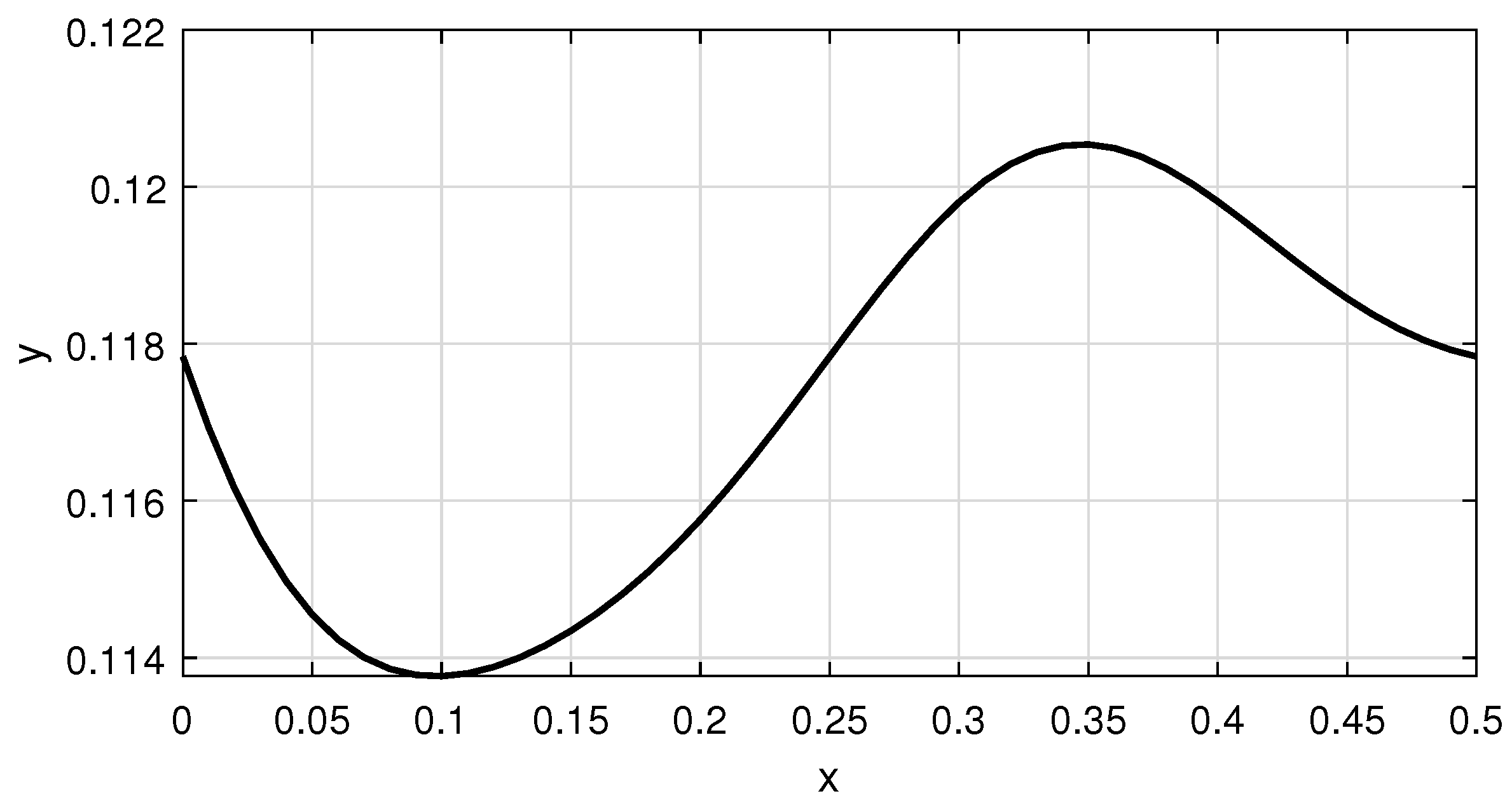
Appendix B. The MATLAB R2022a Code Used for Generating Figure 3

function Example2_3bvp(solver)
% Check for pasting of character " ’ " (<=PDF conversion of code)
% Use vertical single quotation mark instead of right single quotation
mark !
if nargin < 1
solver = ’bvp4c’;
end
bvpsolver = fcnchk(solver);
% Initial mesh - duplicate the interface point xc
xc=0.25;
xinit = [0, 0.01, 0.02, 0.03, 0.04, 0.05, 0.06, 0.07, 0.08, 0.09, 0.10,
0.11, 0.12, 0.13, 0.14, 0.15, 0.16, 0.17, 0.18, 0.19, 0.20, 0.21, 0.22,
0.23, 0.24, xc, xc, 0.26, 0.27, 0.28, 0.29, 0.30, 0.31, 0.32, 0.33, 0.34,
0.35, 0.36, 0.37, 0.38, 0.39, 0.40, 0.41, 0.42, 0.43, 0.44, 0.45, 0.46,
0.47, 0.48, 0.49, 0.50];
% all points in "xinit" must be in one line !!!
yinit = [0.0; -1.0];
sol = bvpinit(xinit,yinit);
sol = bvpsolver(@f,@bc,sol);
plot(sol.x,sol.y(1,:),’k’,’LineWidth’,1.5)
pbaspect([2 1 1])
xlabel(’x’); ylabel(’y’); grid on
print(’Figure_3’,’-deps’)  % output -> Figure_3.eps
function dydx = f(x,y,region)
  dydx = zeros(2,1);
  dydx(1)=y(2); % y(1) = y and y(2) = y’
switch region
case 1
dydx(2)=0.75*atan(y(1))*(1+sin(y(2)))+(cos(3*pi*x))^3+2*(y(1));
case 2
dydx(2)=0.75*atan(y(1))*(1+sin(y(2)))+(cos(3*pi*x))^3+2*(y(1));
   otherwise
   error(’MATLAB:threebvp3:BadRegionIndex’,’Incorrect region index:%d’,
   region);
end
  end
  % -----------------------------------------------------------------------
  % Boundary conditions
    function res=bc(YL,YR)
   res=[YR(1,1)-YL(1,1)   % the first boundary condition  y1/4(1)-y0(1)=0
        YR(1,1)-YL(1,2)   % continuity of y(1) at xc=1/4
        YR(2,1)-YL(2,2)   % continuity of y(2) at xc=1/4
        YR(1,2)-YL(1,2)]; % the second boundary condition y1/2(1)-y1/4(1)=0
  end
  % -----------------------------------------------------------------------
end

References

  1. Ingram, S.K. Continuous dependence on parameters and boundary data for nonlinear two-point boundary value problems. Pac. J. Math. 1972, 41, 395–408. [Google Scholar] [CrossRef] [Green Version]
  2. Vasiliev, N.I.; Klokov, J.A. Foundations of the Theory of Boundary Value Problems for Ordinary Differential Equations; Zinatne: Riga, Latvia, 1978. (In Russian) [Google Scholar]
  3. Idczak, D. Stability in semilinear problems. J. Differ. Equ. 2000, 162, 64–90. [Google Scholar] [CrossRef] [Green Version]
  4. Jones, C.K.R.T. Geometric Singular Perturbation Theory. In Dynamical Systems, Part of the Lecture Notes in Mathematics; Springer: Heidelberg, Germany, 2006; Volume 1609, pp. 44–118. [Google Scholar]
  5. Fenichel, N. Geometric singular perturbation theory for ordinary differential equations. J. Differ. Equ. 1979, 31, 53–98. [Google Scholar] [CrossRef] [Green Version]
  6. Wiggins, S. Normally Hyperbolic Invariant Manifolds in Dynamical Systems; Springer Science+Business Media: New York, NY, USA, 1994. [Google Scholar]
  7. Kuehn, C. Multiple Time Scale Dynamics; Springer: Cham, Switzerland; Heidelberg, Germany; New York, NY, USA; Dordrecht, The Netherlands; London, UK, 2015. [Google Scholar]
  8. Riley, J.W. Fenichel’s Theorems with Applications in Dynamical Systems; University of Louisville: Louisville, KY, USA, 2012. [Google Scholar]
  9. Vasil’eva, A.B. Asymptotic Behavior of Solutions of Problems for Ordinary Nonlinear Differential Equations with a Small Parameter Multiplying the Highest Derivatives, Russian Math. Surveys 1963, 18, 13–84. [Google Scholar]
  10. Vasil’eva, A.B.; Butuzov, V.F. Asymptotic Expansions of Solutions of Singularly Perturbed Equations; Nauka: Moscow, Russia, 1973. (In Russian) [Google Scholar]
  11. De Coster, C.; Habets, P. Two-Point Boundary Value Problems: Lower and Upper Solutions; Elsevier Science: Amsterdam, The Netherlands, 2006. [Google Scholar]
  12. Chang, K.W.; Howes, F.A. Nonlinear Singular Perturbation Phenomena: Theory and Applications; Springer: New York, NY, USA, 1984. [Google Scholar]
  13. Vrabel, R. Upper and lower solutions for singularly perturbed semilinear Neumann’s problem. Math. Bohem. 1997, 122, 175–180. [Google Scholar] [CrossRef]
  14. Vrabel, R. On the approximation of the boundary layers for the controllability problem of nonlinear singularly perturbed systems. Syst. Control Lett. 2012, 61, 422–426. [Google Scholar] [CrossRef] [Green Version]
  15. Nagumo, M. Über die Differentialgleichung y=f(x,y,y). Proc. Phys. Math. Soc. Jpn. 1937, 19, 861–866. [Google Scholar]
  16. Jackson, L.K. Subfunctions and Second-Order Ordinary Differential Inequalities. Adv. Math. 1968, 2, 308–363. [Google Scholar] [CrossRef] [Green Version]
  17. Fabry, C.; Mawhin, J.; Nkashama, M.N. A multiplicity result for periodic solutions of forced nonlinear second order ordinary differential equations. Bull. London Math. Soc. 1986, 18, 173–180. [Google Scholar] [CrossRef]
  18. Hartman, P. Ordinary Differential Equations; Society for Industrial and Applied Mathematics (Classics in Applied Mathematics): Philadelphia, PA, USA, 2002. [Google Scholar]
  19. Bernstein, S.N. Sur les équations du calcul des variations. Ann. Sci. Ecole Norm. Sup. 1912, 29, 431–485. [Google Scholar] [CrossRef] [Green Version]
  20. Granas, A.; Guenther, R.B.; Lee, J.W. Nonlinear boundary value problems for some classes of ordinary differential equations. Rocky Mt. J. Math. 1980, 10, 35–58. [Google Scholar] [CrossRef]
  21. Granas, A.; Guenther, R.B.; Lee, J.W. On a theorem of S. Bernstein. Pac. J. Math. 1978, 74, 67–82. [Google Scholar] [CrossRef] [Green Version]
  22. Šeda, V. On some non-linear boundary value problems for ordinary differential equations. Arch. Math. 1989, 25, 207–222. [Google Scholar]
  23. Schmitt, K. A nonlinear boundary value problem. J. Differ. Equ. 1970, 7, 527–537. [Google Scholar] [CrossRef]
  24. EMORY, Oxford College. Available online: https://mathcenter.oxford.emory.edu/site/math111/proofs/rollesTheorem/ (accessed on 10 June 2023).
Figure 1. Solution of the BVP y = ( sin 2 π x ) y 3 + ω y + x 2 + 1 , 0 < x < 1 , (2) (left) and (3) (right) for ω = 6 , which implies that | y ( x ) | M 0 = 2 / ω = 1 / 3 in the interval [ 0 , 1 ] on the basis of Lemma 3.
Mathematics 11 02717 g001
Figure 2. Solution of the BVP y = ( sin 2 π x ) y 3 + ω y + x 2 + 1 , 0 < x < 1 , (4) ( c = 1 / 2 ) (left) and (5) ( c = d = 1 / 2 ) (right) for ω = 6 , which implies that | y ( x ) | M 0 = 2 / ω = 1 / 3 in the interval [ 0 , 1 ] on the basis of Lemma 3.
Mathematics 11 02717 g002
Figure 3. Solution of the BVP (11), (12) → y ( 0 ) = y ( 1 / 4 ) = y ( 1 / 2 ) = 0.1178 .
Mathematics 11 02717 g003
Figure 4. Solution of the SPBVP ε y = [ y sin 4 π x ] 3 ,   y ε ( 1 / 4 ) y ε ( 0 ) = 0 ,   y ε ( 1 / 2 ) y ε ( 1 / 4 ) = 0 , for ε = 10 2 (left), ε = 10 3 (right). The dashed line shows the function u ( x ) = sin 4 π x , the solution of the reduced problem.
Mathematics 11 02717 g004
Figure 5. Solution of the SPBVP ε y = [ y sin 4 π x ] 3 ,   y ε ( 1 / 4 ) y ε ( 0 ) = 0 ,   y ε ( 1 / 2 ) y ε ( 1 / 4 ) = 0 , for ε = 10 4 (left), ε = 10 5 (right).
Mathematics 11 02717 g005
Figure 6. Solution of the SPBVP ε y = [ y sin 4 π x ] 3 ,   y ε ( 1 / 4 ) y ε ( 0 ) = 0 ,   y ε ( 1 / 2 ) y ε ( 1 / 4 ) = 0 , for ε = 10 6 (left), ε = 10 7 (right).
Mathematics 11 02717 g006
Figure 7. Solution of the SPBVP (18), (4) for ε = 10 2 (left), ε = 10 1 (right). The dashed line shows the function u ( x ) = 2 + cos x ,   x [ 0 , 3 π / 2 ] , the solution of the reduced problem.
Mathematics 11 02717 g007
Figure 8. Solution of the SPBVP (18), (4) for ε = 10 1 .
Mathematics 11 02717 g008
Disclaimer/Publisher’s Note: The statements, opinions and data contained in all publications are solely those of the individual author(s) and contributor(s) and not of MDPI and/or the editor(s). MDPI and/or the editor(s) disclaim responsibility for any injury to people or property resulting from any ideas, methods, instructions or products referred to in the content.

