A New Estimator: Median of the Distribution of the Mean in Robustness

Abstract

In some statistical methods, the statistical information is provided in terms of the values used by classical estimators, such as the sample mean and sample variance. These estimations are used in a second stage, usually in a classical manner, to be combined into a single value, as a weighted mean. Moreover, in many applied studies, the results are given in these terms, i.e., as summary data. In all of these cases, the individual observations are unknown; therefore, computing the usual robustness estimators with them to replace classical non-robust estimations by robust ones is not possible. In this paper, the use of the median of the distribution $F_{\overline{x}}$ of the sample mean is proposed, assuming a location-scale contaminated normal model, where the parameters of $F_{\overline{x}}$ are estimated with the classical estimations provided in the first stage. The estimator so defined is called median of the distribution of the mean, $MdM$. This new estimator is applied in Mendelian randomization, defining the new robust inverse weighted estimator, RIVW.

1. Introduction

In the application of some statistical methods, such as clinical trials, the results are, usually, described in terms of the values taken by classical estimators, such as the sample mean and sample variance. These results are combined, in a second stage, as a weighted mean in a meta analysis. The same occurs in its alternative, Mendelian Randomization, one of the main topics in causal inference.

Moreover, in many applied studies, their results have been described in these terms, i.e., as summary data, not knowing the individual observations, to compute robust estimators with them, replacing the classical non-robust estimations with robust ones.

In this paper, a solution to this problem is proposed, correcting, if necessary, the given classical estimations because, although the individual observations are unknown, the mechanism that generates the data is known because it is the model.

Focusing on the mean estimation problem, the optimal estimator (uniformly minimum variance unbiased estimator) is the sample mean, when no outliers exist in the sample, and the normal distribution $N(\mu ,{\sigma }^2)$ is assumed as the model, with $\mu$ and ${\sigma }^2$ being the usual parameters of the normal distribution, population mean, and variance. Assume that a proportion $ϵ$ of outliers exists in the sample, i.e., a contaminated normal model (see [1], p. 2)

$$(1-ϵ)N(\mu ,{\sigma }^2)+ϵN(g_1\mu ,g_2^2{\sigma }^2)$$

where most of the data are from a $N(\mu ,{\sigma }^2)$, and a small part of them, $ϵ$, are from a normal model with more dispersion and a different location, $N(g_1\mu ,g_2^2{\sigma }^2)$, where $g_1$ is a contamination parameter that affects the location, and $g_2$ is a contamination parameter that affects the scale. The optimality of the sample mean is lost because the optimal procedure and its properties heavily depend on the assumed probability model ([2], p. 2). This is the reason why classical statistics rests, basically, on the normal model and on the sample mean.

Additionally, under a contaminated normal model, the robustness of the sample mean is lost [1,3]. Under this model, the sample mean is not the maximum likelihood estimator [4], and even the normality of the sample mean is not guaranteed [5].

In this paper, a new estimator for a location–scale contaminated normal model is proposed, avoiding the extreme sensitivity of the sample mean but coinciding with it when no outliers are present in the data. The median of the distribution $F_{\overline{x}}$ of the sample mean is proposed as a new estimator, where the parameters of $F_{\overline{x}}$ are estimated with the classical estimations described in previous studies. This estimator is called the median of the distribution of the mean, $MdM$.

The two reasons why this new estimator relies on the distribution of the sample mean are that, first, the classical estimations are given in terms of the classical mean (and classical variance) and, second, this new procedure extends the classical one in the sense that if no outliers are present, this new estimator is the classical sample mean, i.e., with this method, the classical estimation is extended to the case in which outliers are present.

Another estimator somewhat related to $MdM$ is the median of the means estimator $MoM$. However, this estimator is, finally, one of the sample means and, hence, is not robust (see [6]).

With the $MdM$, robustness and optimality are obtained if there are no outliers. Hence, with this approach, a new vision of the dilemma between optimality and robustness is provided.

Because the exact sample distribution of $\overline{x}$ under a mixture distribution is not known, here it is estimated in a closed form with the von Mises (VOM) plus saddlepoint (SAD) method, a technique used by the author in several studies (see, for instance, [7,8]) but in another context. With this approximation, the estimator introduced in this paper can also be extended to other more general models than the normal mixture considered here.

The rest of the paper is structured as follows. In Section 2, the VOM+SAD approximation for the distribution of the sample mean is obtained under a location–scale contaminated normal model. The definition and some properties of this new location estimator are considered in Section 3, and a scale estimator, based on these ideas, is defined in Section 4, and an example of the application of this new estimator is considered in Section 5. These ideas are applied to Mendelian randomization in Section 6. Some conclusions are outlined in Section 7.

2. VOM+SAD Approximation of Sample Mean Distribution

Because the new estimator depends on the distribution of the sample mean, the distribution of the sample mean must be very precise, especially when the considered sample sizes are very small. For this situation, using a von Mises expansion ([9], p. 215, or [10], p. 578) that depends on Hampel’s influence function [11] is highly recommended.

Although, in the end, the obtained results are be applied to the mixture of normals model considered previously, these refer to more general models, F, G, and H, which indicate future extensions of this method.

The final approximation is called VOM+SAD and was previously obtained by the author in the context of spatial data (see [7,8]). Following the ideas developed in those two papers, considering the tail probability functional, initially, the approximation obtained is

$$P_F\{T_n>t\}\simeq P_G\{T_n>t\}+\int \mathrm{TAIF}\left(x;t;T_n,G\right)dF\left(x\right)$$

which allows the approximation of the distribution of $T_n$ when the observations follow model F by the distribution of $T_n$ when the variables of $T_n$ follow model G (pivotal distribution).

This approximation depends on the tail area influence function, TAIF, defined in [12].

Restricting this approximation to M estimators with a monotonic decreasing score function $\psi$ (see [1], p. 46) and using the Lugannani and Rice formula ([13], or [14] p. 77, or [1] p. 314) to obtain a saddlepoint approximation for the TAIF, as the approximation given in [15] (p. 94), for M estimators, the VOM+SAD approximation obtained is

$$P_F\{T_n>t\}\simeq P_G\{T_n>t\}+\int \frac{\varphi \left(s\right)}{r_1}{n}^{1/2}\left(\frac{e^{z_0\psi (x,t)}}{\int e^{z_0\psi (y,t)}dG\left(y\right)}-1\right)dF\left(x\right).$$

In the case of a location–scale mixture normal model, the framework that it is considered in this paper, i.e., assuming that $Z_i\equiv (1-ϵ)N(\mu ,{\sigma }^2)+ϵN(g_1\mu ,g_2^2{\sigma }^2)$, the VOM+SAD approximation is

$$P_F\{T_n>t\}\simeq P_G\{T_n>t\}+ϵ\frac{\varphi \left(s\right)}{r_1}\sqrt{n}\left(\frac{\int e^{z_0\psi (x,t)}dH\left(x\right)}{\int e^{z_0\psi (y,t)}dG\left(y\right)}-1\right)$$

(1)

where $G=N(\mu ,{\sigma }^2)$, and $H=N(g_1\mu ,g_2^2{\sigma }^2)$.

VOM-SAD Approximation for the Distribution of the Sample Mean

In the particular case of the sample mean, the score function is $\psi (x,t)=x-t$. Remember that in the VOM+SAD approximation, the saddlepoint is computed under $G=N(\mu ,{\sigma }^2)$. Under this pivotal distribution, it is

$$K(\lambda ,t)=log\int e^{\lambda (y-t)}\frac{1}{\sigma \sqrt{2\pi }}{e}^{-\frac{1}{2{\sigma }^2}{(y-\mu )}^2}dy=\frac{{\sigma }^2{\lambda }^2}{2}+\lambda (\mu -t).$$

Hence, from the saddlepoint equation $K^{\prime }(z_0,t)=0$ the saddlepoint $z_0=(t-\mu )/{\sigma }^2$ is obtained.

Additionally, $K(z_0,t)=-{(t-\mu )}^2/\left(2{\sigma }^2\right)$, $\varphi \left(s\right)=\varphi (\sqrt{n}(t-\mu )/\sigma )$, $r_1=(t-\mu )/\sigma$, and $K^{″}(\lambda ,t)={\sigma }^2$. The leading term is $P_G\{T_n>t\}=1-\Phi (\sqrt{n}(t-\mu )/\sigma )$, and the quotient in last term in the right side of (1) is

$$\frac{\int e^{z_0\psi (x,t)}dH\left(x\right)}{\int e^{z_0\psi (y,t)}dG\left(y\right)}=exp\left\{(g_1-1)\mu z_0+\frac{1}{2}(g_2^2-1)\sigma z_0^2\right\}.$$

Hence, the VOM+SAD approximation (1) is

$$P_F\{\overline{x}>t\}\simeq 1-\Phi \left(\sqrt{n}\sigma z_0\right)+ϵ\frac{\sqrt{n}}{\sigma z_0}\varphi \left(\sqrt{n}\sigma z_0\right)\left(e^{(g_1-1)\mu z_0+\frac{1}{2}(g_2^2-1)\sigma z_0^2}-1\right).$$

If distributions F and G are not close enough, intermediate distributions can be considered, as in [16,17,18], to obtain a more accurate approximation.

3. Estimator Median of the Distribution of the Mean

If the previous distribution of the mean is

$$F_{\overline{x}}\left(x\right)=1-P_F\{\overline{x}>x\}$$

the median of this distribution, i.e., $F_{\overline{x}}^{-1}(1/2)$, is called the median of the distribution of the mean, $MdM$, i.e., this estimator is the solution of

$$F_{\overline{x}}\left(MdM\right)=\frac{1}{2}.$$

The parameters of $F_{\overline{x}}$ are estimated with the classical estimations, the sample mean $\overline{x}$ and the sample variance $s^2$.

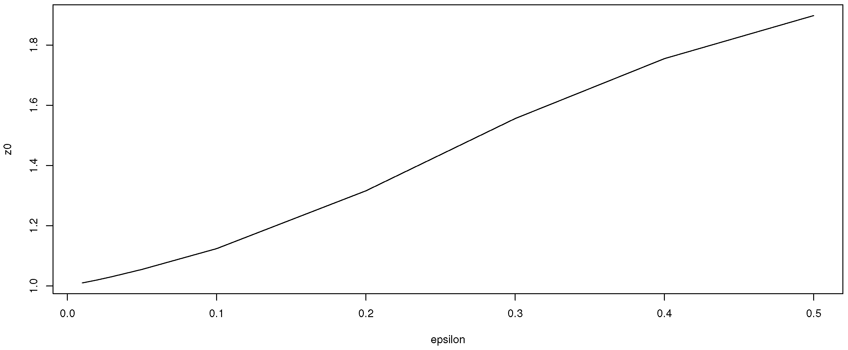
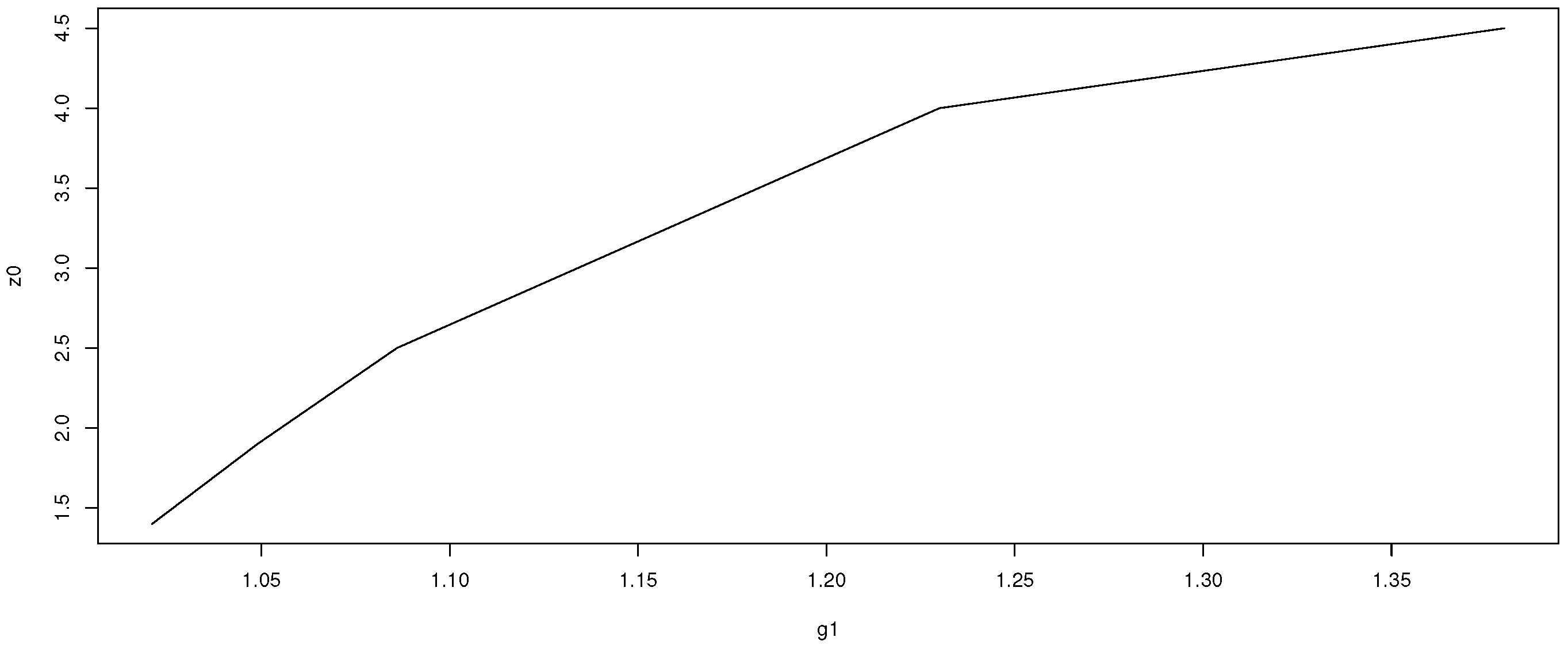
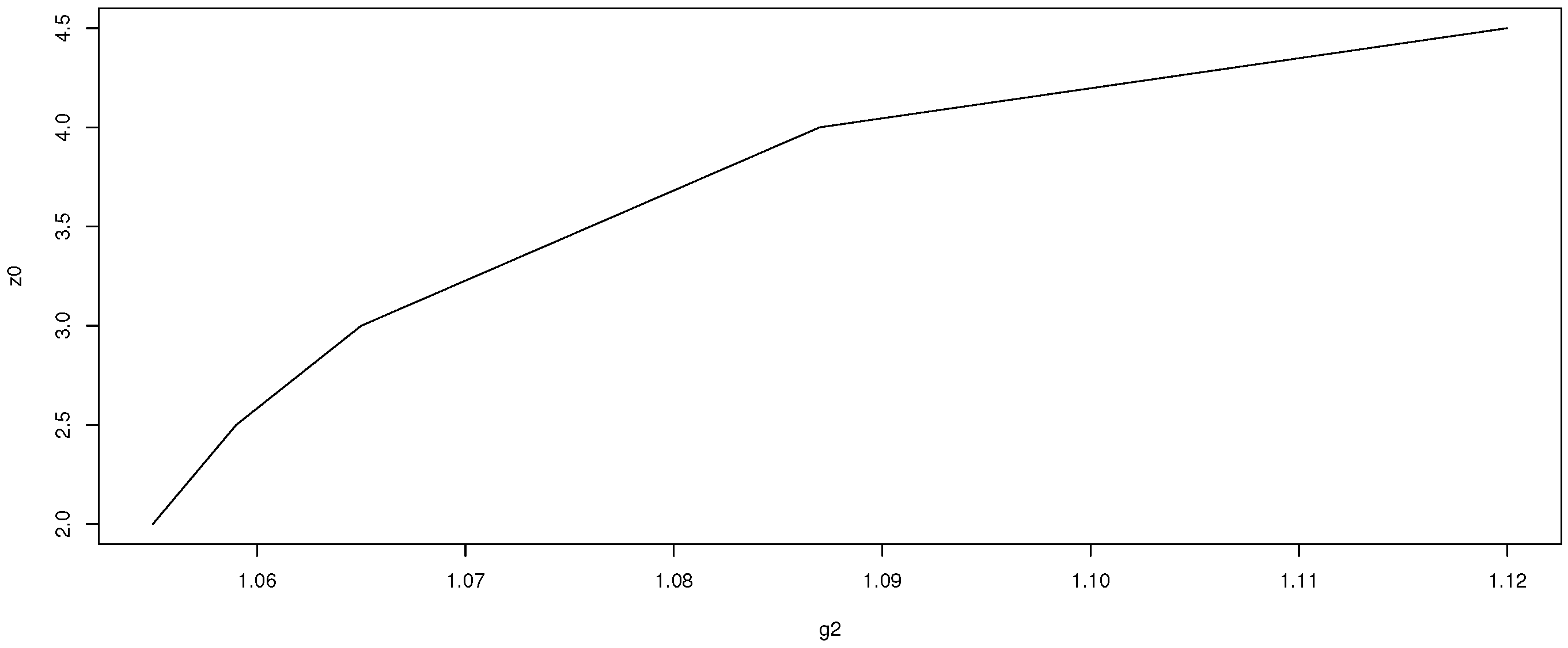
Figure 1, Figure 2 and Figure 3 show that as contamination parameters $ϵ$, $g_1$, or $g_2$ increase, the difference between $MdM$ and $\overline{x}$, i.e., $z_0$, increases.

Figure 1. Differences between $MdM$ and $\overline{x}$ as $ϵ$ increases.

Figure 2. Differences between $MdM$ and $\overline{x}$ as $g_1$ increases.

Figure 3. Differences between $MdM$ and $\overline{x}$ as $g_2$ increases.

The main reason for the definition of $MdM$ is that the median is more robust than the sample mean and, hence, the influence of possible outliers, not knowing the individual observations, as assumed here, should be lower with the median of the distribution of the mean than with the sample mean, used in this distribution as an estimator of the location parameter. Furthermore, in the case without outliers, this estimator is equal to the classical sample mean.

As a limitation, observe that $MdM$ is also sensitive if outliers already affect the sample mean or sample variance used in the estimation of the location or scale parameter $\mu$ or ${\sigma }^2$. Nevertheless, with $MdM$, this sensitivity is lower.

One way to check the behavior of $MdM$ with respect to $\overline{x}$ in a simple numerical example is to run the R sentences

> 

x<-0.80*rnorm(11,2,1)+0.2*rnorm(11,3*2,1)

> 

mean(x)

> 

median(x)

in which we consider a random sample of $n=11$ sample data from a mixture normal $0.8N(2,1)+0.2N(3·2,1)$, i.e., a sample where $ϵ=0.2,g_1=3$ and $g_2=1$.

Finally, in future research, other robust estimators could be considered, such as the trimmed mean of the distribution of the sample mean.

4. Dispersion Estimator

With the ideas developed in this paper, a dispersion estimator should be

$$F_{\overline{x}}^{-1}(3/4)-F_{\overline{x}}^{-1}(1/4).$$

5. Example

In most application papers, only the final values of the estimators used on them are given. Additionally, these estimators are usually the classical sample mean and sample variance and do not include the individual observations from which these estimators are obtained and, therefore, not providing the opportunity to robustify these values using robust techniques.

For this reason, a large number of examples could serve as an illustration of the estimator defined in this paper. Next, let us consider just one.

Example 1.

One of these studies is [19], where some vertebral column and thorax of Neanderthals fossils were re-evaluated using their vertebrae because, probably, as stated by the author, errors occurred in the reconstruction and the samples were wrongly classified. He mentions ([19], p. 23) a misclassification of 7/33, which can be considered as the value of the contamination parameter ϵ.

Because modern humans and Neanderthals have very similar vertebrae, no difference in the mean is assumed, using, hence a distortion factor $g_1=1$. On the other hand, Neanderthals are slightly more stockier than modern humans, with the dispersion of the latter being larger, assuming that $g_2=1.5$.

In Table 2 in [19], classical acceptance confidence intervals are provided for several vertebrae of 28 modern humans. They are based on the classical mean and variance, as the author says in this table. From the table, with respect vertebra T1, the remains of Kebara 2 and La Ferrassie can be considered as modern humans instead of Neanderthals, because they are inside of the confidence interval. The same happens with vertebra T7 but not with vertebra T5.

From these classical intervals, for vertebra T1, the classical sample mean and standard deviation are $\overline{x}=16.6$ and $S=3.61$, respectively. In this case, the estimator median of the distribution of the mean takes the value $MdM=15.034$, obtaining the new robust acceptance confidence interval equal to $[13.63,16.43]$, which does not contain the remains, concluding then, that these remains are Neanderthals and not modern humans, as they were wrongly considered with the classical estimators.

With respect to vertebra T5, $MdM=17.54$, and the new robust acceptance confidence interval is $[15.84,19.24]$, with neither the classical nor the robust interval not including the remains, confirming that they are Neanderthals.

Finally, for vertebra T7, $MdM=19.43$, and the new robust acceptance confidence interval $[17.73,21.13]$, both this robust and the previous classical confidence interval including the remains of the La Ferrassie, hence being modern humans and not Neanderthals.

6. Robust Inverse-Weighted Estimator RIVW in Mendelian Randomization

Another field for the class of problems considered in this paper is randomized clinical trials (CTs). In each of these CTs, the sample mean and sample variance are the usual final result. These are usually combined, in a classical way, as a weighted mean in a meta-analysis. In CTs, the relationship of a variable X (called cause) with another variable Y (called effect) is analyzed, but reverse causality may exist or a lack complete randomization or, more importantly, confounders may be present.

Moreover, CTs are expensive and take a long time. With Mendelian randomization (MR), a method that has received a renewed interest in recent years, CTs are imitated because, in any person, all genetic material is randomized allocated from their parents, including DNA markers. Randomly, some people receive more DNA markers related with variable X and, for others, fewer. MR uses genetic variants (usually single-nucleotide polymorphisms (SNPs)) as instrumental variables Z.

Mathematically, MR is used to avoid possible biases in the regression of Y on X due to these three causes just mentioned. Formally, MR leads us to a two-step linear regression process; first, for every genetic variant $Z_j,j=1,\dots ,L$, a linear regression of X on $Z_j$ is performed, where, for individuals, $i=1,\dots ,n_j$ is

$$X_i\mid Z_{ij}={\beta }_{X_0}+{\beta }_{X_j}{Z}_{ij}+e_{X_{ij}}$$

from which the fitted values ${\widehat{X}}_i$ are obtained and used in a second regression of Y on these $\widehat{X}$, obtaining finally [20]

$$Y_i\mid Z_{ij}={\beta }_{Y_0}+(\beta ·{\beta }_{X_j}+{\alpha }_j)Z_{ij}+e_{Y_{ij}}={\beta }_{Y_0}+{\beta }_{Y_j}{Z}_{ij}+e_{Y_{ij}}$$

where ${\beta }_{X_j}$ and ${\beta }_{Y_j}$ represent the association of $Z_j$ with the exposure and the outcome (only through X), respectively. The parameter $\beta ·{\beta }_{X_j}$ represents the effect of $Z_j$ on Y through X, where $\beta$ is the causal effect of X on Y that is being estimated. Moreover, ${\alpha }_j$ represents the association between $Z_j$ and Y not through the exposure of interest. Finally, the errors terms $e_{X_{ij}}$ and $e_{Y_{ij}}$ are assumed to be independent because independent samples are assumed to be used to fit the two previous regression models.

In MR, the standard estimator of the parameter of interest $\beta$, the slope in the linear regression of Y on X, is the classical two-stage least squares estimator

$${\widehat{\beta }}_{R_j}=\frac{{\widehat{\beta }}_{Y_j}}{{\widehat{\beta }}_{X_j}}$$

which is the quotient of the slope of the regression of Y on $Z_j$, ${\widehat{\beta }}_{Y_j}$, and the slope estimator of the regression of X on $Z_j$, ${\widehat{\beta }}_{X_j}$. These classical estimations, one for each value of the instrumental variable $Z_j$, are combined with the classical inverse-variance weighted (IVW) estimator

$$\mathrm{IVW}=\sum _{j=1}^L{\omega }_j{\widehat{\beta }}_{R_j}/(\sum _{j=1}^L{\omega }_j)$$

where ${\omega }_j=1/var({\widehat{\beta }}_{R_j})$, which is used to weight the ${\widehat{\beta }}_{R_j}$ estimators, assuming that the L genetic variants are mutually independent. In this way, a single causal effect estimate from L genetic instruments is obtained.

This classic and widely used estimator is not robust because it has a $0\%$ breakdown point because it is a weighted mean, see, for instance, [21].

In this section, the robustification of the classical estimator IVW is obtained, first, by replacing estimators ${\widehat{\beta }}_{R_j}$ with the median of the distribution of the mean, $Md{M}_j$ estimators and, second, by replacing the weights ${\omega }_j$ with $v_j$, the inverse of the new dispersion estimator,

$$v_j=\frac{1}{F_{\overline{x}}^{-1}(3/4)-F_{\overline{x}}^{-1}(1/4)}$$

defining the new estimator, based on the ${\widehat{\beta }}_{R_j}$ distribution, as

$$\mathrm{RIVW}=\frac{{\sum }_{j=1}^L{v}_{j}Md{M}_j}{{\sum }_{j=1}^L{v}_j}.$$

6.1. Distribution of ${\widehat{\beta }}_{R_j}$ Estimator

In this section, an approximation for the distribution of ${\widehat{\beta }}_{R_j}$ is obtained for each genetic variant $Z_j,j=1,\dots ,L$, i.e, j is fixed. Moreover, because of the usual regression assumptions, $Z_{ij}$ is not random in the two previous linear regressions, i.e., in the estimator ${\widehat{\beta }}_{R_j}$.

Hence, with ${\mu }_{X_i}$ denoting the constant

$${\mu }_{X_i}={\beta }_{X_0}+{\beta }_{X_j}{Z}_{ij}$$

avoiding the j in the notation of ${\mu }_{X_i}$ to simplify it, and with ${\mu }_{Y_i}$ being the constant

$${\mu }_{Y_i}={\beta }_{Y_0}+{\beta }_{Y_j}{Z}_{ij},$$

and assuming no outliers in the sample, the variable $X_i\mid Z_{ij}$ follows a normal distribution

$$X_i\mid Z_{ij}\equiv N({\mu }_{X_i},{\sigma }_{X_i}^2)$$

and

$$Y_i\mid Z_{ij}\equiv N({\mu }_{Y_i},{\sigma }_{Y_i}^2).$$

The estimator ${\widehat{\beta }}_{R_j}$ is equal to

$${\widehat{\beta }}_{R_j}=\frac{{\widehat{\beta }}_{Y_j}}{{\widehat{\beta }}_{X_j}}$$

and, considering standardized data, i.e., that ${\widehat{\beta }}_{R_j}$ is computed as a correlations quotient,

$${\widehat{\beta }}_{R_j}=\frac{{\displaystyle \sum _{i=1}^{n_j}{Y}_i{Z}_{ij}}}{{\displaystyle \sum _{i=1}^{n_j}{X}_i{Z}_{ij}}}$$

its tail distribution is

$$\begin{array}{ccc}\hfill P\left\{{\widehat{\beta }}_{R_j}>a\right\}& =& P\left\{\frac{{\sum }_{i=1}^{n_j}{Y}_i{Z}_{ij}}{{\sum }_{i=1}^{n_j}{X}_i{Z}_{ij}}>a\right\}\hfill \\ & =& P\left\{\sum _{i=1}^{n_j}{Y}_i{Z}_{ij}-a\sum _{i=1}^{n_j}{X}_i{Z}_{ij}>0\right\}\hfill \\ & =& P\left\{\sum _{i=1}^{n_j}(Y_i-a{X}_i)Z_{ij}>0\right\}.\hfill \end{array}$$

Letting $W_i$ (removing the j if there is no risk of confusion) denote the random variable $W_i=W_{ij}=(Y_i-a{X}_i)Z_{ij}$, $i=1,\dots ,n_j$, where a and $Z_{ij}$ are not random, the aim is to compute the distribution of the sample mean of the variables $W_i$ at 0, i.e.,

$$P\left\{{\widehat{\beta }}_{R_j}>a\right\}=P\left\{\sum _{i=1}^{n_j}{W}_i>0\right\}=P\left\{\overline{W}>0\right\}$$

where $W_i$ is independent but not identically distributed because

$$W_i\mid Z_{ij}\equiv N({\mu }_i,{\sigma }_i^2),i=1,\dots ,n_j$$

where

$${\mu }_i=({\mu }_{Y_i}-a·{\mu }_{X_i})Z_{ij}$$

and

$${\sigma }_i^2=V\left((Y_i-a·X_i)Z_{ij}\right)$$

which depends on ${\sigma }_{X_i}^2$ and ${\sigma }_{Y_i}^2$. The values of these parameters are given from previous studies following the median of the distribution the mean method.

If the data contain no outliers, it will be

$$W_i\mid Z_{ij}\equiv N({\mu }_i,{\sigma }_i^2)$$

but, as usual, a proportion $ϵ$ of outliers in the data is assumed, i.e., as a model for the observations $W_i$ the following

$$F_i=(1-ϵ)N({\mu }_i,{\sigma }_i^2)+ϵN(g_{i1}{\mu }_i,g_{i2}^2{\sigma }_i^2)$$

where the contamination constants $g_{i1}$ and $g_{i2}$ are assumed to depend on $i=1,\dots ,n_j$.

To compute the distribution of $\overline{W}$ under models $F_i$, assuming that the sample sizes $n_j$ are small, a von Mises approximation (VOM), based on a von Mises expansion, is used to obtain an accurate approximation with small sample sizes.

6.2. VOM Approximation of the Distribution

In general, to approximate the tail probability of statistic $T_n$ under a vector of model distributions $\mathbf{F}=(F_1,\dots ,F_n)$, knowing its tail distribution under the vector of model distributions $\mathbf{G}=(G_1,\dots ,G_n)$ (called pivotal distributions), the von Mises expansion of the tail probability of $T_n({\mathbf{X}}_1,{\mathbf{X}}_2,\dots ,{\mathbf{X}}_n)$ at $\mathbf{F}$ is used ([10], Section 2, or [22], Theorem 2.1, or [17], Corollary 2),

$$P_{\mathbf{F}}\{T_n({\mathbf{X}}_1,{\mathbf{X}}_2,\dots ,{\mathbf{X}}_n)>t\}=P_{F_1,\dots ,F_n}\{T_n({\mathbf{X}}_1,{\mathbf{X}}_2,\dots ,{\mathbf{X}}_n)>t\}$$

$$=P_{\mathbf{G}}\{T_n({\mathbf{X}}_1,{\mathbf{X}}_2,\dots ,{\mathbf{X}}_n)>t\}+\sum _{i=1}^n{\int }_{\mathcal{X}}{\mathrm{TAIF}}_i\left(\mathbf{x};t;T_n,\mathbf{G}\right)d{F}_i\left(\mathbf{x}\right)+Rem$$

where the sample space $\mathcal{X}\subset {\mathbb{R}}^m$,

$$Rem=\frac{1}{2}{\int }_{\mathcal{X}}{\int }_{\mathcal{X}}{T}_{{\mathbf{G}}_{\mathbf{F}}}^{\left(2\right)}({\mathbf{x}}_1,{\mathbf{x}}_2)d\left[\mathbf{F}\left({\mathbf{x}}_{\mathbf{1}}\right)-\mathbf{G}\left({\mathbf{x}}_{\mathbf{1}}\right)\right]d\left[\mathbf{F}\left({\mathbf{x}}_{\mathbf{2}}\right)-\mathbf{G}\left({\mathbf{x}}_{\mathbf{2}}\right)\right]$$

where $T_{{\mathbf{G}}_{\mathbf{F}}}^{\left(2\right)}$ is the second derivative of the tail probability functional at the mixture distribution ${\mathbf{G}}_{\mathbf{F}}=(1-\lambda )\mathbf{G}+\lambda \mathbf{F}$, for some $\lambda \in [0,1]$; and ${\mathrm{TAIF}}_i$ is the ith (multivariate) partial tail area influence function of $T_n$ at $\mathbf{G}=(G_1,\dots ,G_n)$ in relation to $G_i$, $i=1,\dots ,n$, introduced in [17], Definition 1,

$${\displaystyle {\mathrm{TAIF}}_i(\mathbf{x};t;T_n,\mathbf{G})=\frac{\partial }{\partial ϵ}{P}_{G_i^{ϵ,\mathbf{x}}}\{T_n({\mathbf{X}}_1,\dots ,{\mathbf{X}}_n)>t\}{\mid }_{ϵ=0}}$$

in those $\mathbf{x}\in \mathcal{X}$ where the right-hand side exists. In the computation of ${\mathrm{TAIF}}_i$, only $G_i$ is contaminated; the other distributions remain fixed, $i=1,\dots ,n$.

In general, $Rem$ is close to 0, and the von Mises approximation (VOM) is defined as

$$\begin{array}{ccc}\hfill P_{\mathbf{F}}\{T_n({\mathbf{X}}_1,{\mathbf{X}}_2,\dots ,{\mathbf{X}}_n)>t\}& \simeq & P_{\mathbf{G}}\{T_n({\mathbf{X}}_1,{\mathbf{X}}_2,\dots ,{\mathbf{X}}_n)>t\}\hfill \\ & & +\sum _{i=1}^n{\int }_{\mathcal{X}}{\mathrm{TAIF}}_i\left(\mathbf{x};t;T_n,\mathbf{G}\right)d{F}_i\left(\mathbf{x}\right).\hfill \end{array}$$

(2)

Moreover, if $\mathbf{F}$ is a mixture distribution, $\mathbf{F}=(1-ϵ)\mathbf{G}+ϵ\mathbf{H}$, $Rem=O\left({ϵ}^2\right)$ ([23], p. 77). Additionally, because of the partial influence functions properties ([22], p. 3) that are valid for the partial tail area influence functions defined in [17], for any $T_n$ it will be

$${\int }_{\mathcal{X}}{\mathrm{TAIF}}_i\left(\mathbf{x};t;T_n,\mathbf{G}\right)d{G}_i\left(x\right)=0,$$

(3)

i.e., the integral with respect a given model of the ${\mathrm{TAIF}}_i$ that depends on this model is equal to 0. Hence,

$$P_{\mathbf{F}}\{T_n({\mathbf{X}}_1,{\mathbf{X}}_2,\dots ,{\mathbf{X}}_n)>t\}=P_{\mathbf{G}}\{T_n({\mathbf{X}}_1,{\mathbf{X}}_2,\dots ,{\mathbf{X}}_n)>t\}$$

$$+(1-ϵ)\sum _{i=1}^n{\int }_{\mathcal{X}}{\mathrm{TAIF}}_i\left(\mathbf{x};t;T_n,\mathbf{G}\right)d{G}_i\left(\mathbf{x}\right)$$

$$+ϵ\sum _{i=1}^n{\int }_{\mathcal{X}}{\mathrm{TAIF}}_i\left(\mathbf{x};t;T_n,\mathbf{G}\right)d{H}_i\left(\mathbf{x}\right)+O\left({ϵ}^2\right)$$

$$=P_{\mathbf{G}}\{T_n({\mathbf{X}}_1,{\mathbf{X}}_2,\dots ,{\mathbf{X}}_n)>t\}+0+ϵ\sum _{i=1}^n{\int }_{\mathcal{X}}{\mathrm{TAIF}}_i\left(\mathbf{x};t;T_n,\mathbf{G}\right)d{H}_i\left(\mathbf{x}\right)+O\left({ϵ}^2\right)$$

i.e., the VOM approximation is

$$P_{\mathbf{F}}\{T_n({\mathbf{X}}_1,{\mathbf{X}}_2,\dots ,{\mathbf{X}}_n)>t\}\simeq P_{\mathbf{G}}\{T_n({\mathbf{X}}_1,{\mathbf{X}}_2,\dots ,{\mathbf{X}}_n)>t\}$$

$$+ϵ\sum _{i=1}^n{\int }_{\mathcal{X}}{\mathrm{TAIF}}_i\left(\mathbf{x};t;T_n,\mathbf{G}\right)d{H}_i\left(\mathbf{x}\right).$$

Moreover, because of Proposition 1 in [17],

$$\begin{array}{ccc}\hfill {\mathrm{TAIF}}_i\left(\mathbf{x};t;T_n,\mathbf{G}\right)& =& -P_{G_1,\dots ,G_n}\{T_n({\mathbf{X}}_1,{\mathbf{X}}_2,\dots ,{\mathbf{X}}_n)>t\}\hfill \\ & & \\ & +& P_{G_1,\dots ,G_{i-1},G_{i+1},\dots ,G_n}\{T_n({\mathbf{X}}_1,\dots ,{\mathbf{X}}_{i-1},\mathbf{x},{\mathbf{X}}_{i+1},\dots ,{\mathbf{X}}_n)>t\}\hfill \end{array}$$

and the VOM approximation of the tail probability $P_{\mathbf{F}}\{T_n({\mathbf{X}}_1,{\mathbf{X}}_2,\dots ,{\mathbf{X}}_n)>t\}$ can also be expressed as

$$\begin{array}{ccc}\hfill P_{\mathbf{F}}\{T_n({\mathbf{X}}_1,{\mathbf{X}}_2,\dots ,{\mathbf{X}}_n)>t\}& \simeq & (1-n)P_{\mathbf{G}}\{T_n({\mathbf{X}}_1,{\mathbf{X}}_2,\dots ,{\mathbf{X}}_n)>t\}\hfill \\ & & +{\int }_{\mathcal{X}}{P}_{G_2,\dots ,G_n}\{T_n(\mathbf{x},{\mathbf{X}}_2,\dots ,{\mathbf{X}}_n)>t\}d{F}_1\left(\mathbf{x}\right)\hfill \\ & & +{\int }_{\mathcal{X}}{P}_{G_1,G_3,\dots ,G_n}\{T_n({\mathbf{X}}_1,\mathbf{x},\dots ,{\mathbf{X}}_n)>t\}d{F}_2\left(\mathbf{x}\right)+\cdots \hfill \\ & & +{\int }_{\mathcal{X}}{P}_{G_1,\dots ,G_{n-1}}\{T_n({\mathbf{X}}_1,\dots ,{\mathbf{X}}_{n-1},\mathbf{x})>t\}d{F}_n\left(\mathbf{x}\right)\hfill \end{array}$$

(4)

which allows an approximation of the tail probability $P_{\mathbf{F}}\{T_n({\mathbf{X}}_1,{\mathbf{X}}_2,\dots ,{\mathbf{X}}_n)>t\}$ under models $\mathbf{F}=(F_1,\dots ,F_n)$, knowing the value of this tail probability under near models $\mathbf{G}=(G_1,\dots ,G_n)$.

In the particular case that $T_n({\mathbf{X}}_1,{\mathbf{X}}_2,\dots ,{\mathbf{X}}_n)=\overline{W}$, the VOM approximation for the tail of $\overline{W}$ can be expressed as (see (2) with $n=n_j,j=1,\dots ,L$ and $t=0$ now)

$$P_{\mathbf{F}}\left\{\overline{W}>0\right\}\simeq P_{\mathbf{G}}\{W_1+\dots +W_{n_j}>0\}+\sum _{i=1}^{n_j}{\int }_{\mathbb{R}}{\mathrm{TAIF}}_i\left(x;0;\overline{W},\mathbf{G}\right)d{F}_i\left(x\right)$$

or, see (4),

$$P_{\mathbf{F}}\left\{\overline{W}>0\right\}\simeq P_{\mathbf{G}}\{W_1+\dots +W_{n_j}>0\}$$

$$+\sum _{i=1}^{n_j}{\int }_{\mathbb{R}}\left[-P_{\mathbf{G}}\{W_1+\dots +W_{n_j}>0\}\right.$$

$$\left.+P_{G_1,\dots ,G_{i-1},G_{i+1},\dots ,G_{n_j}}\{W_1+\dots +W_{i-1}+x+W_{i+1}+\dots +W_{n_j}>0\}d{F}_i\left(x\right)\right]$$

or

$$\begin{array}{ccc}\hfill P_{\mathbf{F}}\left\{\overline{W}>0\right\}& \simeq & (1-n_j)P_{\mathbf{G}}\{W_1+\dots +W_{n_j}>0\}\hfill \\ & & +{\int }_{\mathbb{R}}{P}_{G_2,\dots ,G_{n_j}}\{x+W_2+\dots +W_{n_j}>0\}d{F}_1\left(x\right)\hfill \\ & & +{\int }_{\mathbb{R}}{P}_{G_1,G_3,\dots ,G_{n_j}}\{W_1+x+W_3+\dots +W_{n_j}>0\}d{F}_2\left(x\right)+\dots \hfill \\ & & +{\int }_{\mathbb{R}}{P}_{G_1,\dots ,G_{i-1},G_{i+1},\dots ,G_{n_j}}\{W_1+\dots +W_{i-1}+x+W_{i+1}+\dots +W_{n_j}>0\}d{F}_i\left(x\right)\hfill \\ & & +\dots +{\int }_{\mathbb{R}}{P}_{G_1,\dots ,G_{n_j-1}}\{W_1+\dots +W_{n_j-1}+x>0\}d{F}_{n_j}\left(x\right).\hfill \end{array}$$

If it is assumed as model for the observations $W_i$

$$F_i=(1-ϵ)N({\mu }_i,{\sigma }_i^2)+ϵN(g_{i1}{\mu }_i,g_{i2}^2{\sigma }_i^2)$$

and it is denoted by $G_i^{g_{i1},g_{i2}}\equiv N(g_{i1}{\mu }_i,g_{i2}^2{\sigma }_i^2)$, and by $G_i\equiv N({\mu }_i,{\sigma }_i^2)$ the pivotal distribution, $i=1,\dots ,n_j$, i.e.,

$$F_i=(1-ϵ)G_i+ϵG_i^{g_{i1},g_{i2}}.$$

the generic component of this last equation is

$${\int }_{\mathbb{R}}{P}_{G_1,\dots ,G_{i-1},G_{i+1},\dots ,G_{n_j}}\{W_1+\dots +W_{i-1}+x+W_{i+1}+\dots +W_{n_j}>0\}d{F}_i\left(x\right)=$$

$${\int }_{\mathbb{R}}{P}_{G_1,\dots ,G_{i-1},G_{i+1},\dots ,G_{n_j}}\{W_1+\dots +W_{i-1}+W_{i+1}+\dots +W_{n_j}>-x\}d{F}_i\left(x\right)$$

$$={\int }_{\mathbb{R}}\left[1-\Phi \left(\frac{-x-{\mu }_{-i}}{{\sigma }_{-i}}\right)\right]d{F}_i\left(x\right)$$

where $\Phi$ is the cumulative distribution function of a standard normal distribution,

$${\mu }_{-i}={\mu }_1+\dots +{\mu }_{i-1}+{\mu }_{i+1}+\dots +{\mu }_{n_j}$$

and

$${\sigma }_{-i}^2={\sigma }_1^2+\dots +{\sigma }_{i-1}^2+{\sigma }_{i+1}^2+\dots +{\sigma }_{n_j}^2.$$

If

$${\mu }_s={\mu }_1+\dots +{\mu }_{n_j}={\mu }_{-i}+{\mu }_i$$

and

$${\sigma }_s^2={\sigma }_1^2+\dots +{\sigma }_{n_j}^2={\sigma }_{-i}^2+{\sigma }_i^2$$

then,

$$P_{\mathbf{G}}\{W_1+\dots +W_{n_j}>0\}=1-\Phi \left(\frac{-{\mu }_s}{{\sigma }_s}\right)$$

and

$$P_{\mathbf{F}}\left\{{\widehat{\beta }}_{R_j}>a\right\}=P_{\mathbf{F}}\left\{\sum _{i=1}^{n_j}{W}_i>0\right\}=P_{\mathbf{F}}\left\{\overline{W}>0\right\}$$

$$\simeq 1-\Phi \left(\frac{-{\mu }_s}{{\sigma }_s}\right)+\sum _{i=1}^{n_j}{\int }_{\mathbb{R}}\left[\Phi \left(\frac{-{\mu }_s}{{\sigma }_s}\right)-\Phi \left(\frac{-x-{\mu }_{-i}}{{\sigma }_{-i}}\right)\right]d{F}_i\left(x\right).$$

(5)

Because $F_i$ is a normal mixture

$$F_i=(1-ϵ)G_i+ϵG_i^{g_{i1},g_{i2}}$$

the VOM approximation (5) is

$$=1-\Phi \left(\frac{-{\mu }_s}{{\sigma }_s}\right)+ϵ\sum _{i=1}^{n_j}{\int }_{\mathbb{R}}\left[\Phi \left(\frac{-{\mu }_s}{{\sigma }_s}\right)-\Phi \left(\frac{-x-{\mu }_{-i}}{{\sigma }_{-i}}\right)\right]d{G}_i^{g_{i1},g_{i2}}\left(x\right).$$

Moreover, because of property (3) for the partial influence functions mentioned before, it is

$${\int }_{\mathbb{R}}\left[\Phi \left(\frac{-{\mu }_s}{{\sigma }_s}\right)-\Phi \left(\frac{-x-{\mu }_{-i}}{{\sigma }_{-i}}\right)\right]d{G}_i\left(x\right)=0$$

or

$${\int }_{\mathbb{R}}\Phi \left(\frac{-x-{\mu }_{-i}}{{\sigma }_{-i}}\right)d{G}_i\left(x\right)=\Phi \left(\frac{-{\mu }_s}{{\sigma }_s}\right).$$

Hence, making the change of variable $(x+{\mu }_{-i})/{\sigma }_{-i}=y$, it is

$${\int }_{\mathbb{R}}\Phi \left(\frac{-x-{\mu }_{-i}}{{\sigma }_{-i}}\right)d{G}_i^{g_{i1},g_{i2}}\left(x\right)=\Phi \left(\frac{-{\mu }_s^{g_{i1}}}{{\sigma }_s^{g_{i2}}}\right)$$

where

$${\mu }_s^{g_{i1}}={\mu }_1+\dots +{\mu }_{i-1}+g_{i1}{\mu }_i+{\mu }_{i+1}+\dots +{\mu }_{n_j}$$

and

$${\sigma }_s^{g_{i2}}=\sqrt{{\sigma }_1^2+\dots +{\sigma }_{i-1}^2+g_{i2}{\sigma }_i^2+{\sigma }_{i+1}^2+\dots +{\sigma }_{n_j}^2}.$$

Then, the VOM approximation to the distribution of ${\widehat{\beta }}_{R_j}$ is

$$P\left\{{\widehat{\beta }}_{R_j}>a\right\}=1-\Phi \left(\frac{-{\mu }_s}{{\sigma }_s}\right)+ϵ\sum _{i=1}^{n_j}\left[\Phi \left(\frac{-{\mu }_s}{{\sigma }_s}\right)-\Phi \left(\frac{-{\mu }_s^{g_{i1}}}{{\sigma }_s^{g_{i2}}}\right)\right].$$

Example 2.

In a study [24], whether low-density lipoprotein cholesterol (LDL-C) is a cause of coronary artery disease (CAD) was analyzed considering 28 DNA markers

• DNA markers X Y
• SNP exposure.beta exposure.se outcome.beta outcome.se
• 1 snp_1 0.0260 0.004 0.0677 0.0286
• 2 snp_2 -0.0440 0.004 -0.1625 0.0300
• ..............................................................
• 27 snp_27 0.0090 0.003 0.0000 0.0255
• 28 snp_28 -0.0360 0.007 0.0198 0.0647

Usually, $Z_i\equiv B(2,0.5)$ is assumed to be an instrumental variable to mimic biallelic SNPs in Hardy–Weinberg equilibrium. A value

$$IVW=2.834214$$

was obtained.

With the method proposed in this paper, considering sample sizes of $n=37$, $n_1=17$, $n_2=10$, and $n_3=10$, and contamination parameters $ϵ=0.05$, $g_{i1}=1$, and $g_{i2}=1.5$, for the first DNA marker is obtained

$${\mu }_s={\mu }_1+\dots +{\mu }_{n_j}=30\times (0.0677-a\times 0.0260)$$

$${\sigma }_i^2=0.0286\times 37=1.0582$$

$${\sigma }_s=\sqrt{1.0582\times 37}=6.257268$$

$${\mu }_s^{g_{i1}}={\mu }_s$$

and

$${\sigma }_s^{g_{i2}}=\sqrt{{\sigma }_1^2+\dots +{\sigma }_{i-1}^2+g_{i2}{\sigma }_i^2+{\sigma }_{i+1}^2+\dots +{\sigma }_{n_j}^2}$$

$$=\sqrt{1.0582\times 36+1.5\times 1.0582}=6.299405$$

$$Md{M}_1=2.59$$

$$v_1=\frac{1}{F_{\overline{x}}^{-1}(3/4)-F_{\overline{x}}^{-1}(1/4)}=\frac{1}{8.08-(-2.877)}=0.0912.$$

For all the 28 DNA markers, we have

$$\begin{array}{ccccccc}Md{M}_j\hfill & 2.59& 3.70& 2.78& 2.71& 4.93& \dots \\ v_j\hfill & 0.091& 0.151& 0.128& 0.088& 0.068& \dots \end{array}$$

which are combined in the new robust estimate

$$RIVW=2.042703.$$

7. Conclusions

In this paper, a new method for estimating the parameters in a location–scale contamination model is introduced, in the case where individual observations are not available and, therefore, applying the usual robust methods is not possible, i.e., in summary data problems.

For the location problem, a new estimator was defined that is equal to the usual sample mean when no outliers exist and correcting classical estimations when outliers exist.

This new estimator was applied to one of the most used estimators in Mendelian randomization, the inverse-variance weighted estimator (IVW), defining a new estimator robust inverse weighted estimator (RIVW).