Exploring Initialization Strategies for Metaheuristic Optimization: Case Study of the Set-Union Knapsack Problem

Abstract

In recent years, metaheuristic methods have shown remarkable efficacy in resolving complex combinatorial challenges across a broad spectrum of fields. Nevertheless, the escalating complexity of these problems necessitates the continuous development of innovative techniques to enhance the performance and reliability of these methods. This paper aims to contribute to this endeavor by examining the impact of solution initialization methods on the performance of a hybrid algorithm applied to the set union knapsack problem (SUKP). Three distinct solution initialization methods, random, greedy, and weighted, have been proposed and evaluated. These have been integrated within a sine cosine algorithm employing k-means as a binarization procedure. Through testing on medium- and large-sized SUKP instances, the study reveals that the solution initialization strategy influences the algorithm’s performance, with the weighted method consistently outperforming the other two. Additionally, the obtained results were benchmarked against various metaheuristics that have previously solved SUKP, showing favorable performance in this comparison.

1. Introduction

Over the past few years, metaheuristic methods have emerged as powerful tools in addressing complex problems, particularly those pertaining to the realm of combinatorial challenges. A wide array of applications across various fields, including biology [1,2], logistics [3], civil engineering [4,5], machine learning [6], and many more, serve as compelling evidence of their effectiveness in problem-solving.

These methods have garnered considerable attention owing to their capacity to effectively navigate extensive search spaces and identify near-optimal solutions within relatively brief timeframes. This characteristic has demonstrated its particular value in addressing the immense scale and complexity inherent in numerous combinatorial problems. The ability to find satisfactory solutions for complex problems in a time-efficient manner has solidified the importance of these methods in the field of optimization.

However, as the intricacy of such problems continues to grow, the challenges associated with efficiently solving them also intensify. Consequently, there is a pressing need for innovative techniques and strategies that can enhance the performance of these methods, ensuring that they remain relevant and effective when confronted with increasingly complex optimization tasks. The development of advanced algorithms and the integration of novel approaches in the initialization process can contribute to overcoming these obstacles, ultimately bolstering the performance and reliability of these methods in tackling large-scale, intricate combinatorial problems.

In response to these challenges, researchers have focused on the development and application of diverse approaches aimed at enhancing and fortifying metaheuristic algorithms. One notable example involves hybrid techniques, which amalgamate the strengths of various metaheuristic algorithms. By integrating complementary methods and harnessing their synergies, these hybrid techniques have demonstrated success in augmenting the overall performance, accuracy, and efficiency of the underlying metaheuristic algorithms. Another intriguing aspect to explore is the examination of the forms and parameters of solution initialization.

The significance of initialization operators lies in the fact that the diversity and nature of the initial population have an impact on the algorithm’s performance, potentially leading to enhanced solutions and improved convergence rates. Furthermore, the sensitivity of the algorithms is problem-dependent, signifying that the choice of an initialization method can have a substantial influence on the performance for certain problems. In addition, the population size and the number of iterations also play a role in the algorithms’ performance, necessitating an appropriate population size and a sufficient number of iterations to achieve optimal solutions. Lastly, the effectiveness of initialization methods varies depending on the specific metaheuristic optimizer employed, making it crucial to comprehend the relationship between initialization methods and optimizers in order to select the most suitable combination for specific problems. In summary, good population diversity and an adequate number of iterations, combined with an appropriate initialization method, are likely to lead to optimal solutions.

In the literature exploration, it has been observed that studies such as [7] compare the effects of population size, maximum iterations, and eleven initialization methods on the convergence and accuracy of metaheuristic optimizers. Results have indicated that sensitivity to initialization schemes varies among algorithms and is problem-dependent. Furthermore, performance has been found to rely on population size and the number of iterations, with greater diversity and a suitable quantity of iterations being more likely to produce optimal solutions. In a study by [8], a systematic comparison of 22 initialization methods was conducted, analyzing their impact on the convergence and accuracy of five optimizers: DE, PSO, CS, ABC, and GA. The findings revealed that 43.37% of DE functions and 73.68% of PSO and CS functions were significantly affected by initialization methods. Population size, number of iterations, and certain probability distributions also influenced performance.

In the study by [9], a reliability-analysis-based structural shape optimization formulation was proposed, incorporating Latin hypercube sampling (LHS) as the initialization scheme. The investigation focused on the relationship between geometry and fatigue life in structural component design. The extended finite element method (XFEM) and level set description were utilized, and nature-inspired optimization techniques were employed to solve the problems. Results indicated that proper shape changes can enhance the service life of structural components subjected to fatigue loads, with the location and orientation of initial imperfections significantly affecting optimal shapes. Finally, in [10], the authors provided an extensive review of diverse initialization strategies designed to improve the performance of metaheuristic optimization algorithms. Emphasizing the crucial role of initialization, various distribution schemes, population sizes, and iteration numbers have been investigated by researchers in pursuit of optimal solutions. Notable schemes encompass random numbers, quasirandom sequences, chaos theory, probability distributions, hybrid algorithms, Lévy flights, and more. Additionally, the paper evaluated the influence of population size, maximum iterations, and ten distinct initialization methods on three prominent population-based metaheuristic optimizers: bat algorithm (BA), grey wolf optimizer (GWO), and butterfly optimization algorithm (BOA).

Aligning with the process of solution initialization, this paper proposes various strategies for initializing solutions, incorporating these strategies into a discrete hybrid algorithm detailed in [11]. This algorithm merges the concept of k-means with metaheuristics and is applied to the set union knapsack problem (SUKP). The SUKP [12] is an extended version of the traditional knapsack problem and has attracted considerable research interest in recent years [13,14,15]. This attention is primarily due to its intriguing applications [16,17], coupled with the complexity and challenge involved in solving it efficiently.

In the context of the SUKP, an assortment of items is identified, each with a specific profit value attributed. Additionally, a correspondence is established between each item and a group of elements, with each carrying a weight that impacts the knapsack constraint. A scrutiny of the existing body of literature reveals that the SUKP is predominantly addressed using advanced metaheuristics, with outcomes provided within acceptable time limits. However, when conventional metaheuristics are utilized in the SUKP, issues including instability and diminished effectiveness are exposed as the instance size increases. For instance, a variety of transfer functions were deployed and evaluated within small to medium SUKP instances, as documented in [18]. A reduction in effectiveness was noted when these algorithms were applied to standard SUKP instances. Adding to the complexity, a new series of benchmark problems have been recently introduced, as noted in [19].

Given these considerations, it becomes imperative to explore solution initialization techniques to assess the algorithm’s performance. The following are the significant contributions of this study:

• Three solution initialization strategies are proposed.
• The initialization solutions are integrated with the SIN-COS metaheuristic and the k-means technique, following the strategy proposed in [20].
• The three initialization strategies are evaluated using medium-sized and large-sized SUKP problems, with the latter being proposed in [19].

The structure of this paper is organized as follows: Section 2 delivers a comprehensive examination of the set-union knapsack problem and its related applications. In Section 3, the k-means sine cosine search algorithm and the initialization operator are thoroughly described. Section 4 expounds on the numerical experiments undertaken and the resulting comparisons. Finally, Section 6 presents concluding insights and explores potential directions for future research.

2. Advancements in Solving the Set-Union Knapsack Problem

The SUKP represents an extended model of a knapsack, which is defined as follows. A set of n elements, denoted as U, is assumed to exist, with each element $j\in U$ possessing a positive weight $w_j$. Assumed also is a set of m items, named V, where each item $i\in V$ is a subset of elements $U_i\subseteq U$ and holds a profit $p_i$. Given the presence of a knapsack with a capacity C, the aim of SUKP is to identify a subset of items $S\subseteq V$ that allows the maximization of the total profit of S, while ensuring that the combined weight of the components belonging to S does not exceed the capacity C of the knapsack. The decision variables of the problem are identified as the elements belonging to the set S. It is noteworthy that an element’s weight is considered only once, even if it corresponds to multiple chosen items in S. The mathematical depiction of SUKP is presented subsequently:

$$\mathrm{Maximize}P\left(S\right)=\sum _{i\in S}{p}_i.$$

(1)

subject to:

$$W\left(S\right)=\sum _{j\in {\cup }_{i\in S}{U}_i}{w}_j\le C,S\subseteq V.$$

(2)

In the research work, interesting applications of SUKP are identified, such as the one introduced in [16]. The aim of this application is the enhancement of robustness and scalability within cybernetic systems. The consideration is given to a centralized cyber system with a fixed memory capacity, which hosts an assortment of profit-generating services (or requests), each inclusive of a set of data objects. The activation of a data object consumes a particular amount of memory; however, recurring utilization of the same data object does not incur additional memory consumption (a pivotal condition of SUKP). The objective involves the selection of a service subset from the pool of available candidates, with the intention to maximize the total profit of these services, whilst keeping the total memory required by the linked data objects within the cyber system’s memory capacity. The SUKP model, in which an item symbolizes a service with its profit and an element represents a data object with its memory usage (element weight), fittingly structures this application. Consequently, the determination of the optimal solution to the resulting SUKP problem parallels the resolution of the data allocation problem.

An additional application worth mentioning relates to the real-time rendering of animated crowds, as noted in [21]. In this study, a method is introduced by the authors to hasten the visualization process for large gatherings of animated characters. A caching system is implemented that permits the reuse of skinned key-poses (elements) in multi-pass rendering, across multiple agents and frames, while endorsing an interpolative approach for key-pose blending. Within this context, each item symbolizes a member of the crowd. More applications are evident in data stream compression using bloom filters, as reported in [17].

SUKP is an $\mathcal{NP}$-hard problem [12], and various methods have been employed to address it. Theoretical studies using greedy approaches or dynamic programming are presented in [12,22]. In [23], an integer linear programming model was developed and applied to small instances comprising 85 and 100 items, yielding optimal solutions.

Metaheuristic algorithms have been employed to tackle SUKP in various studies. In [24], the authors utilize an artificial bee colony technique to address SUKP, integrating a greedy operator to manage infeasible solutions. An enhanced moth search algorithm is developed in [25], incorporating a differential mutation operator to boost efficiency. The Jaya algorithm, along with a differential evolution technique, is applied in [26] to enhance exploration capability. A Cauchy mutation is used to improve exploitation ability, while an enhanced repair operator is designed to rectify infeasible solutions.

In [18], the efficacy of various transfer functions is examined for binarizing moth metaheuristics. A local search operator is devised in [27] and applied to large-scale instances of SUKP. The study proposes three strategies in line with the adaptive tabu search framework, enabling efficient solutions for new SUKP instances. In [28], the grey wolf optimizer (GWO) algorithm is adapted to tackle binary problems. Instead of traditional binarization methods, the study employs a multiple parent crossover with two distinct dominance tactics, replicating GWO’s leadership hierarchy technique. Furthermore, an adaptive mutation featuring an exponentially decreasing step size is employed, aiming to inhibit premature convergence and establish a balance between intensification and diversification.

In [29], the authors merge machine learning and metaheuristics to devise a Q-learning reinforcement strategy for binary optimization problems, using PSO, genetic algorithm, and gbPSO as optimizers. Enhanced optimizers incorporate initial solution generation and a random immigrants mechanism, while a mutation procedure fosters intensified search. This approach is applied to the set-union knapsack problem, producing promising outcomes. Meanwhile, [30] investigates the impact of integrating a backtracking strategy into population-based approaches for the same problem. The proposed method features swarm optimization, an iterative search operator, and a path-relinking strategy for obtaining high-quality solutions. Performance evaluation using benchmark instances demonstrates promising results when compared to existing methods.

3. Initialization, Metaheuristic, and Search Operators

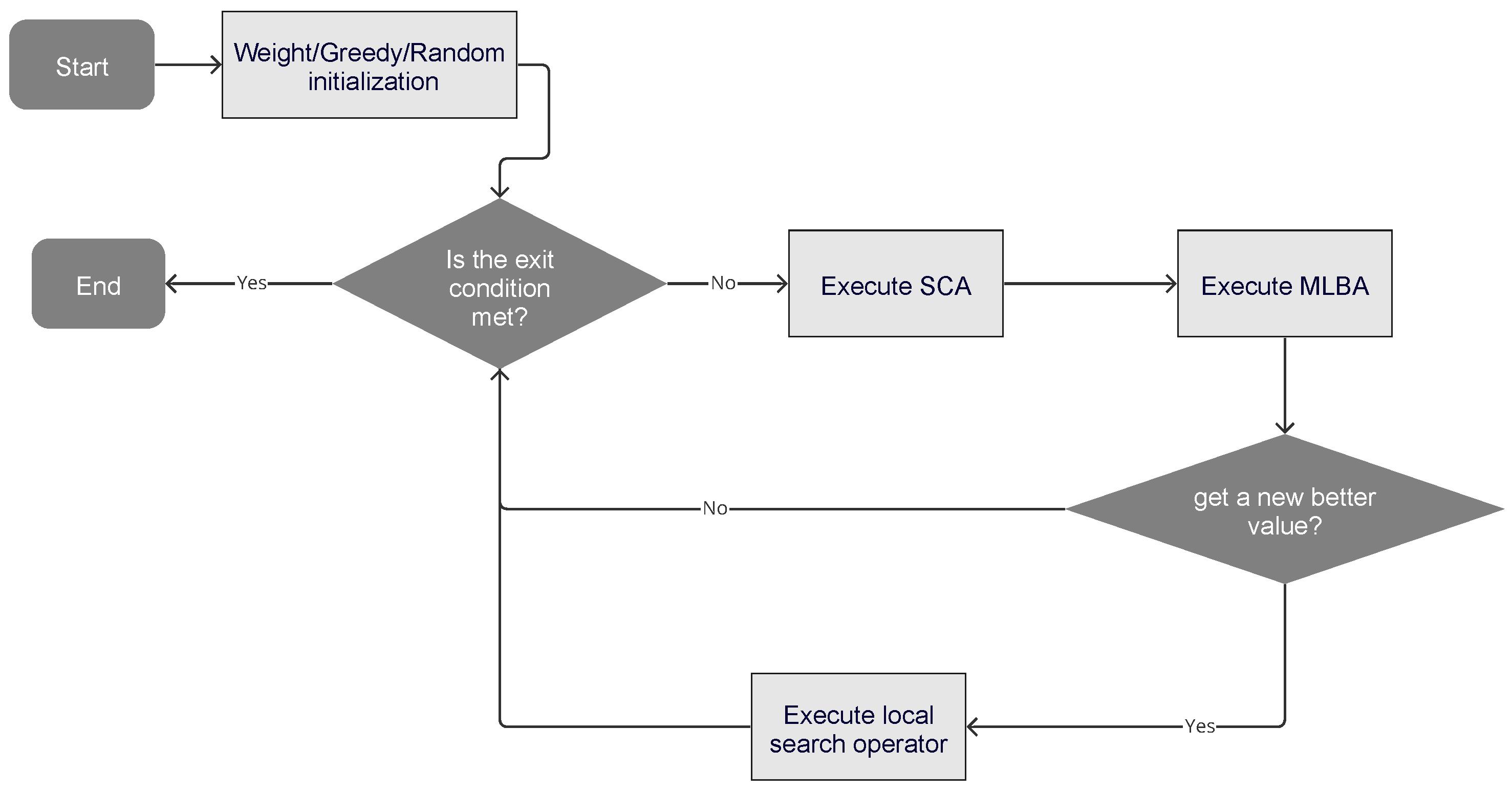
This section outlines a comparison of three distinct initialization operators: a random operator, a greedy operator, and a weighted operator based on a specific indicator. The overall functioning of the proposed algorithm is depicted in Figure 1, with subsequent sections delving into detailed descriptions of each operator. These initialization operators are further elaborated in Section 3.1. Additionally, we discuss the hybrid operator, a unique blend of machine learning techniques and metaheuristics, which is tasked with executing movements. For this study, we implemented a hybrid SCA, as detailed in Section 3.2. Finally, we examine the local search operator, which is utilized to refine the results obtained. This operator is discussed in Section 3.3.

3.1. Initialization Operators

The aim of these operators is to construct the initial solutions that will initiate the search process. To achieve this, items are sorted according to the ratio defined in Equation (3). The operators take $sortItems$ as input, which consists of elements arranged in descending order based on their r values. The output is a valid solution, denoted as Sol.

$$r=\frac{\mathrm{item} \mathrm{profit}}{\mathrm{sum} \mathrm{of} \mathrm{element} \mathrm{weights}}$$

(3)

In the case of the greedy operator, Algorithm 1, at line 4, $Sol$ is initialized with a random element, and this element is removed from the $sortItems$ list. Subsequently, at line 6, the knapsack constraint is checked; if the condition is met, the while loop is entered. Within the loop, a new item is assigned based on Equation (3), and it is removed again from $sortItems$. Once the knapsack is full, the solution requires cleaning in line 10, as its weight is greater than or equal to $knapsackSize$. If the weights are equal, no action is taken. However, if the weight is greater, the items in $Sol$ must be sorted using the r value defined in Equation (3), and removed in ascending order while checking the constraint after each removal. Once the constraint is satisfied, the procedure halts, and the solution $Sol$ is returned.

In the context of the random operator, Algorithm 2, at line 4, a random item is used to initialize $Sol$, and this item is subsequently removed from the $sortItems$ list. Following this, the knapsack constraint is evaluated at line 6. If the condition is fulfilled, the program enters the while loop. Within this loop, a new item is randomly selected without considering the greedy condition and is promptly removed from $sortItems$. When the knapsack is filled, the solution requires adjustment at line 10 as its weight equals or exceeds $knapsackSize$. If the weights are identical, no action is required. However, if the weight of $Sol$ surpasses $knapsackSize$, the items in G must be arranged in accordance with the r-value defined in Equation (3) and are removed in ascending order, with the constraint being evaluated after each removal. The procedure concludes once the constraint is met, returning the solution $Sol$ as the output.

Algorithm 1 Greedy initialization operator.

1: Function initGreedySolutions($sortItems$)   2: Input $sortItems$   3: Output $Sol$   4: $Sol\leftarrow$ getRandom()   5: $sortItems\leftarrow removeFromSortItems(Item$)   6: while (weightSol < knapsackSize) do   7:    $Sol\leftarrow addSortItem(sortItems$)   8:    $sortItems\leftarrow removeFromSortItems(Item$)   9: end while 10: $Sol\leftarrow$ cleanSol($Sol$) 11: return $Sol$ =0

Algorithm 2 Random initial operator.

1: Function initRandomSolutions($sortItems$)   2: Input $sortItems$   3: Output $Sol$   4: $Sol\leftarrow$ getRandom()   5: $sortItems\leftarrow removeFromSortItems(Item$)   6: while (weightSol < knapsackSize) do   7:    $Sol\leftarrow addRandomItem(sortItems$)   8:    $sortItems\leftarrow removeFromSortItems(Item$)   9: end while 10: $Sol\leftarrow$ cleanSol($Sol$) 11: return $Sol$

In the case of the weighted operator, Algorithm 3, the selection process differs in that items are chosen randomly but with a probability governed by Equation (3). In this approach, a normalized probability is constructed for each item, where the sum of all probabilities equals 1. Subsequently, the random selection of items is performed, taking into account the probability assigned to each of them.

Algorithm 3 Weighted initial operator.

1: Function initWeightedSolutions($sortItems$)   2: Input $sortItems$   3: Output $Sol$   4: $Sol\leftarrow$ getRandom()   5: $sortItems\leftarrow removeFromSortItems(Item$)   6: while (weightSol < knapsackSize) do   7:    $Sol\leftarrow addWeightedItem(sortItems$)   8:    $sortItems\leftarrow removeFromSortItems(Item$)   9: end while 10: $Sol\leftarrow$ cleanSol($Sol$) 11: return $Sol$

3.2. Machine Learning Binarization Operator

The binarization process relies heavily on the machine learning binarization algorithm (MLBA). This algorithm receives the list of solutions $lSol$ from the prior iteration, the metaheuristic ($MH$)—in this scenario, SCA, the optimal solution achieved thus far ($bestSol$), and the transition probability for each cluster, $transProbs$, as input. In line 4, the metaheuristic $MH$ is utilized on the list $lSol$; in this specific situation, it corresponds to SCA. The absolute values of velocities $vlSol$ are extracted from the result of applying $MH$ to $lSol$. These velocities symbolize the transition vector obtained through the application of the metaheuristic to the solution list. In line 5, k-means is used to cluster the entire set of velocities (getKmeansClustering); in this particular instance, K is designated as 5. It should be emphasized that the Algorithm 4 in conjunction with Algorithm 5 were proposed in the context of [11].

Algorithm 4 Machine learning binarization operator (MLBA).

1: Function MLBA($lSol$, $MH$, $transProbabs$, $bestSol$)   2: Input $lSol$, $MH$, $transProbabs$   3: Output $lSol$, $bestSol$   4: $vlSol\leftarrow$ getAbsValueVelocities($lSol$, $MH$)   5: $lSolClust\leftarrow$ getKmeansClustering($vlSol$, K)   6: for (each $So{l}_i$ in $lSolClust$) do   7:    for (each $dimSo{l}_{i,j}l$ in $So{l}_i$) do   8:      $dimSolPro{b}_{i,j}$ = getClusterProbability($dimSol$, $transProbabs$)   9:      if $dimSolPro{b}_{i,j}>r_1$ then 10:         Update $lSo{l}_{i,j}$ considering the best. 11:      else 12:         Do not update the item in $lSo{l}_{i,j}$ 13:      end if 14:    end for 15:    $So{l}_i\leftarrow$ cleanSol($So{l}_i$) 16: end for 17: $tempBest\leftarrow$ getBest($lSol$) 18: if $cost\left(tempBest\right)$ > $cost\left(bestSol\right)$ then 19:    $tempBest\leftarrow$ execLocalSearch($tempBest$) 20:    $bestSol\leftarrow$$tempBest$ 21: end if 22: return $lSol$, $bestSol$

Algorithm 5 Local search.

1: Function LocalSearch($bestSol$)   2: Input $bestSol$   3: Output $bestSol$   4: $lsolItems,lsolNoItems\leftarrow$ getItems($bestSol$)   5: i = 0   6: while (i < T) do   7:    $tempSol\leftarrow$ swap($lsolItems$, $lsolNoItems$)   8:    if $profit\left(tempSol\right)>profit\left(bestSol\right)$ and $knapsack\left(tempSol\right)<=knapsackSize$ then   9:      $bestSol\leftarrow tempSol$ 10:    end if 11:    i += 1 12: end while 13: return $bestSol$ =0

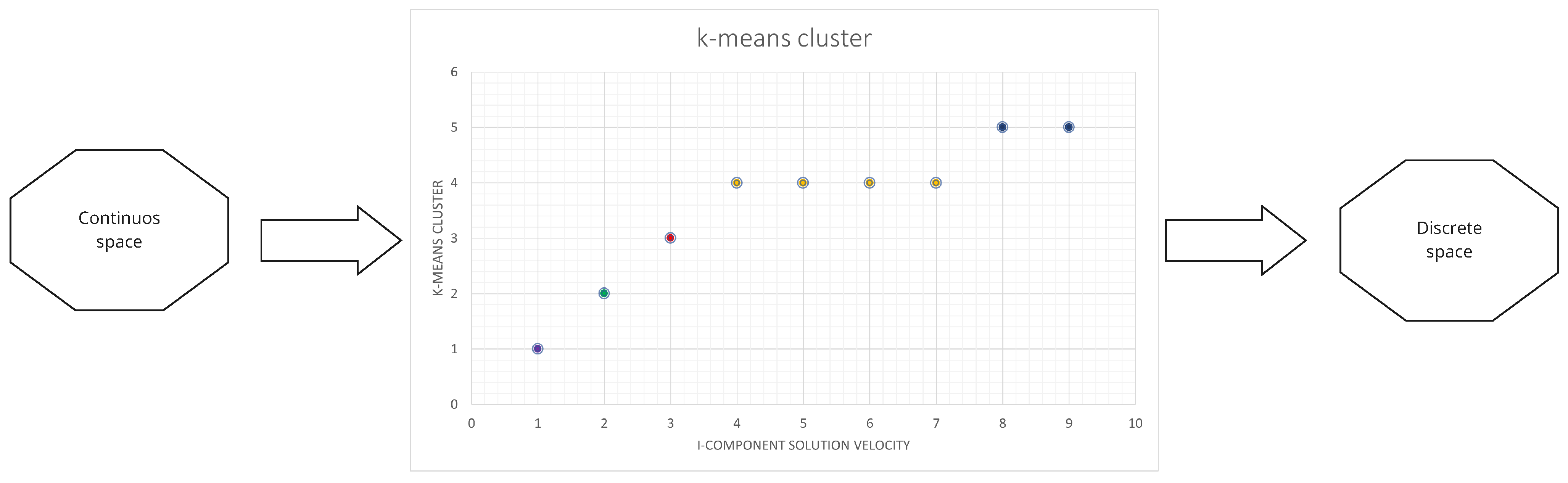
For each solution $So{l}_i$ and dimension j, a cluster assignment is made, and every cluster is linked with a transition probability ($transProbabs$), organized based on the value of the cluster centroid. In this situation, the transition probabilities employed are [0.1, 0.2, 0.4, 0.5, 0.9]. The set of points that belongs to the cluster with the smallest centroid, depicted by the green color in Figure 2, is connected with a transition probability of 0.1. For the collection of blue points with the highest centroid value, a transition probability of 0.9 is associated. The smaller the value of the centroid, the lower the related $transProbs$.

In line 8, for each $lSo{l}_{i,j}$, a transition probability $dimSolPro{b}_{i,j}$ is allocated and subsequently contrasted with a random number $r_1$ in line 9. If $dimSolPro{b}_{i,j}>r_1$, the solution undergoes an update considering the best value in line 10; otherwise, no update occurs, as indicated in line 12. After all solutions have been refreshed, a cleanup process, explained in Section 3.1, is applied. If a new best value emerges, a local search operator is executed in line 19. The details of this local search operator are provided in the following section. Ultimately, the revised list of solutions $lSol$ and the optimal solution $bestSol$ are returned.

3.3. Local Search Operator

The local search operator is invoked whenever a new best value is uncovered by the metaheuristic. This operator accepts the new best values ($bestSol$) as input and, for its initial step, leverages them to ascertain the items that are included and excluded from $bestSol$, as displayed in line 4 of Algorithm 5. These two lists of items undergo an iteration $T=200$ times, effectuating a nonrepetitive swap, as exhibited in line 7 of Algorithm 5. Upon the completion of the swap, two conditions are assessed: whether the profit has improved and if the weight of the knapsack is less than or equal to $knapsackSize$. If both conditions are met, $bestSol$ is updated with $tempSol$, and, ultimately, the refreshed $bestSol$ is returned.

4. Results

This section introduces the experiments performed using MLBA in combination with the sine cosine metaheuristic, aiming to assess the efficacy and contribution of the proposed algorithms when deployed for an $\mathcal{NP}$-hard combinatorial problem. This specific variant of MLBA, which employs the sine cosine algorithm, will be referred to as MLSCABA. The SUKP was elected as a benchmark problem due to its extensive addressal by numerous algorithms and its presentation of nontrivial challenges when it comes to resolving small, medium, and large instances. It should be emphasized that the MLBA binarization technique is highly adaptable to other optimization algorithms. The optimization algorithm of choice was SCA, given its absence of a requirement for parameter tuning and its wide use in solving a variety of optimization problems.

The algorithm was implemented using Python 3.8 and executed on a Windows 10 PC equipped with a Core i7 processor and 32 GB of RAM. To evaluate the statistical significance of the differences, the Wilcoxon signed-rank test was applied with a significance level of 0.05. This test was selected following the methodology delineated in [31]. The Shapiro–Wilk normality test is utilized first in this process. If one of the populations does not adhere to a normal distribution and both populations have an identical number of points, the Wilcoxon signed-rank test is suggested for identifying the difference. In the experiments, the Wilcoxon test was employed to contrast the MLSCABA results with other variants or algorithms used in pairs. A comprehensive list of results was consistently employed for comparisons. The tests were constructed using the statsmodels and scipy libraries in Python. Each instance was solved 30 times to gather the best value and average indicators. Moreover, the average time (in seconds) necessary for the algorithm to discover the optimal solution is documented for each instance.

The initial set of instances, employed during the first phase of this study, were introduced in [32]. These instances encompass between 85 and 500 items and elements. They are distinguished by two parameters. The first parameter, $\mu =\left({\sum }_{i=1}^m{\sum }_{j=1}^n{R}_{ij}\right)/\left(mn\right)$, signifies the density in the matrix, where $R_{ij}=1$ denotes that item i is included in element j. The second parameter, $\nu =C/\left({\sum }_{j=1}^n{w}_j\right)$, denotes the capacity ratio C over the total weight of the elements. As a result, an SUKP instance is labeled as $m\_n\_\mu \_\nu$. The secondary group of instances was proposed in [19] and ranges between 585 and 1000 items and elements. These instances were assembled following the same framework as the preceding set.

4.1. Parameter Setting

The parameter selection was guided by the methodology delineated in [20,33]. This technique draws upon four metrics, encapsulated in Equations (4)–(7), to facilitate judicious parameter selection. We generated values through instances 100_85_0.10_0.75, 100_100_0.15_0.85, and 85_100_0.10_0.75, with each parameter combination undergoing a tenfold validation. The parameters examined and subsequently chosen are documented in

Table 1. Parameter setting for the MLSCABA.

Parameters	Description	Value	Range
N	Number of solutions	10	[5, 10, 20]
K	Clusters number	5	[4, 5]
T	Maximum local search iterations	200	[100, 200, 400]
Transition probability	Transition probability	[0.1, 0.2, 0.4, 0.5, 0.9]	[0.1, 0.2, 0.4, [0.5, 0.6, 0.7], 0.9]

. To identify the optimal configuration, the polygonal area derived from the four-metric radar chart was computed for each setting. The configuration yielding the most expansive area was subsequently selected. Regarding transition probabilities, variation was exclusively confined to the probability of the fourth cluster, assessed at values of [0.5, 0.6, 0.7], while maintaining the rest at a constant level.

• The percentage difference between the best value achieved and the best known value:

  $$bSolution=1-\frac{KnownBestValue-BestValue}{KnownBestValue}$$

  (4)
• The percentage difference between the worst value achieved and the best known value:

  $$wSol=1-\frac{KnownBestValue-WorstValue}{KnownBestValue}$$

  (5)
• The percentage deviation of the obtained average value from the best known value:

  $$aSol=1-\frac{KnownBestValue-AverageValue}{KnownBestValue}$$

  (6)
• The convergence time utilized during the execution:

  $$nTime=1-\frac{convergenceTime-minTime}{maxTime-minTime}$$

  (7)

4.2. Insight into Binary Algorithm

The objective of this section is to have the performance of various initialization operators assessed and compared, specifically random, weighted, and greedy, when applied to two sets of data. In order to carry out this comparison, several key performance indicators were considered, including best value achieved, average value, average execution time, and standard deviation. Valuable insights into the efficiency, effectiveness, and consistency of each initialization operator can be offered by these metrics. To ensure the reliability of the findings, each instance was executed 30 times, providing a more comprehensive evaluation of the performance of the operators across multiple runs.

For the analysis of the results, comparative tables are generated to present quantitative data, box plots are created to facilitate visual comparisons of the performance distributions of the operators, and convergence graphs for selected instances are illustrated to depict the progress of each operator over time. By utilizing these various data visualization techniques, a thorough understanding of the strengths and weaknesses of each initialization operator can be provided, enabling more informed decisions when selecting the most suitable operator for a specific problem or dataset.

The findings from an experimental study on medium-sized instances of the set-union knapsack problem are delineated in

Table 2. Comparison of initialization operators: random, weighted, and greedy for the medium-sized instance set.

		Random				Weighted				Greedy
Instances	Best Known	Best Value	Average	Time (s)	Std	Best Value	Average	Time (s)	Std	Best Value	Average	Time (s)	Std
85_100_0.10_0.75	12,045.00	12,045.00	11,835.33	1.37	193.72	12,045.00	11,866.07	1.22	206.93	12,045.00	11,864.57	1.24	177.94
85_100_0.15_0.85	12,369.00	12,369.00	12,009.37	2.32	392.59	12,369.00	12,043.53	2.52	328.86	12,369.00	11,938.57	2.17	361.75
100_100_0.10_0.75	14,044.00	14,044.00	13,926.97	2.39	92.88	14,044.00	13,882.30	2.34	109.28	14,044.00	13,894.90	3.64	134.65
100_100_0.15_0.85	13,508.00	13,508.00	13,116.07	3.90	239.47	13,508.00	13,174.17	5.46	267.75	13,498.00	12,998.70	3.60	429.24
100_85_0.10_0.75	13,283.00	13,283.00	13,021.87	3.01	154.09	13,283.00	13,029.03	2.42	169.84	13,283.00	12,992.83	3.84	138.88
100_85_0.15_0.85	12,479.00	12,273.00	12,044.77	4.71	203.24	12,479.00	12,015.00	5.96	340.24	12,348.00	12,034.60	3.18	228.98
185_200_0.10_0.75	13,696.00	13,696.00	13,582.93	3.90	101.97	13,696.00	13,559.10	4.64	113.68	13,696.00	13,593.77	5.54	82.97
185_200_0.15_0.85	11,298.00	11,298.00	10,908.87	4.90	248.28	11,298.00	10,923.50	5.64	278.47	11,298.00	10,821.30	4.87	255.41
200_185_0.10_0.75	13,521.00	13,502.00	13,284.00	6.97	176.37	13,502.00	13,287.40	6.56	143.38	13,502.00	13,348.80	7.92	99.57
200_185_0.15_0.85	14,215.00	13,993.00	13,243.17	10.40	479.60	14,215.00	13,234.83	12.84	477.21	13,993.00	13,282.67	9.08	387.88
200_200_0.10_0.75	12,522.00	12,522.00	12,309.57	4.22	183.46	12,522.00	12,262.77	4.37	117.00	12,522.00	12,266.13	7.26	150.87
200_200_0.15_0.85	12,317.00	12,238.00	11,809.53	7.54	230.21	12,317.00	11,842.53	7.00	214.42	12,167.00	11,838.73	11.66	182.89
285_300_0.10_0.75	11,568.00	11,568.00	11,468.43	2.98	86.28	11,568.00	11,495.17	2.54	69.00	11,568.00	11,479.57	3.39	73.66
285_300_0.15_0.85	11,802.00	11,802.00	11,372.00	5.77	205.83	11,802.00	11,411.33	8.18	243.88	11,763.00	11,342.50	6.26	241.63
300_285_0.10_0.75	11,563.00	11,559.00	11,314.17	10.06	143.55	11,563.00	11,346.00	9.05	179.31	11,563.00	11,338.93	7.24	170.56
300_285_0.15_0.85	12,607.00	12,380.00	12,062.07	10.79	300.21	12,402.00	12,084.53	8.04	258.47	12,411.00	12,034.73	10.49	216.47
300_300_0.10_0.75	12,817.00	12,817.00	12,634.20	5.41	93.43	12,817.00	12,652.27	4.83	87.31	12,817.00	12,620.90	4.08	97.47
300_300_0.15_0.85	11,585.00	11,425.00	11,322.17	6.46	140.24	11,425.00	11,288.09	7.88	212.76	11,448.00	11,317.23	7.32	133.51
385_400_0.10_0.75	10,600.00	10,490.00	10,344.23	3.49	74.43	10,600.00	10,357.73	4.69	82.10	10,483.00	10,359.40	4.15	67.64
385_400_0.15_0.85	10,506.00	10,506.00	10,164.50	7.07	153.88	10,506.00	10,175.87	6.72	211.36	10,506.00	10,131.30	7.25	205.12
400_385_0.10_0.75	11,484.00	11,484.00	11,391.97	2.57	89.49	11,484.00	11,409.57	2.82	88.97	11,484.00	11,410.73	2.49	87.33
400_385_0.15_0.85	11,209.00	11,209.00	10,774.00	10.52	292.21	11,209.00	10,725.40	8.82	292.55	11,209.00	10,805.53	11.31	299.81
400_400_0.10_0.75	11,665.00	11,665.00	11,495.67	10.54	141.49	11,665.00	11,501.20	4.21	157.25	11,665.00	11,451.63	4.84	132.43
400_400_0.15_0.85	11,325.00	11,325.00	10,907.23	10.47	422.52	11,325.00	10,976.20	9.24	404.47	11,325.00	10,930.60	8.70	441.57
485_500_0.10_0.75	11,321.00	11,115.00	10,890.13	6.47	106.07	11,260.00	10,885.77	7.73	175.53	11,186.00	10,860.70	7.95	112.53
485_500_0.15_0.85	10,220.00	10,208.00	9835.43	7.70	234.49	10,208.00	9871.23	9.36	215.29	10,208.00	9936.11	7.67	220.54
500_485_0.10_0.75	11,771.00	11,729.00	11,523.77	8.68	151.08	11,729.00	11,504.10	8.64	139.31	11,698.00	11,480.53	8.08	159.68
500_485_0.15_0.85	10,238.00	10,059.00	9834.57	7.23	139.18	10,059.00	9856.20	7.54	111.32	10,086.00	9840.10	7.25	141.35
500_500_0.10_0.75	11,249.00	11,217.00	10,887.07	6.35	120.34	11,123.00	10,854.37	6.08	113.86	11,078.00	10,840.97	6.08	97.11
500_500_0.15_0.85	10,381.00	10,203.00	9931.93	9.08	185.66	10,381.00	9953.77	8.68	261.38	10,381.00	9885.10	7.00	235.07
Average		11,897.07	11,621.47	6.56	185.36	11,928.21	11,627.12	6.51	197.69	11,901.07	11612.11	6.52	186.60
Wilcoxon p-value		0.02	0.02							0.01	0.009

The values highlighted in bold represent the optimal outcomes obtained. It’s important to note that these are only marked when the best result is exclusive to a single algorithm. If there are two algorithms yielding identical optimal values, that instance will not be emphasized.

, with accompanying visualizations depicted in Figure 3 and Figure 4. Three distinct initialization operators—random, greedy, and weighted—were examined in this study. We investigated three different initialization operators, namely, random, greedy, and weighted. The table is formatted in such a way that the first column provides the designation of the instance being analyzed, followed by the column depicting the optimum known solutions for the respective instances. The subsequent four columns illustrate the findings associated with the random initialization operator, including the best-found solution, the average solution, computational time measured in seconds, and the standard deviation of obtained values. In a similar format, the next four columns present the results derived from the weighted operator, while the final quartet of columns elaborate on the outcomes resulting from the application of the greedy operator.

From Table 2, it can be inferred that the best values obtained are associated with the weighted operator, both in terms of best value and average. Additionally, it can be observed that the average convergence times are quite similar among the three operators. The exact number of instances in which the weighted operator outperformed the other two operators in terms of best value was counted, and it was found to be superior in five instances, the random operator in one instance, and the greedy operator in three instances. When the average indicator was analyzed, the weighted initialization operator was observed to outperform the others in 16 instances, while the random operator excelled in seven instances and the greedy operator in seven instances. This further demonstrated the consistent superiority of the weighted operator compared to the others. In the significance analysis, the weighted operator was indicated to be significantly superior to the other two initialization operators, both in terms of best value and average.

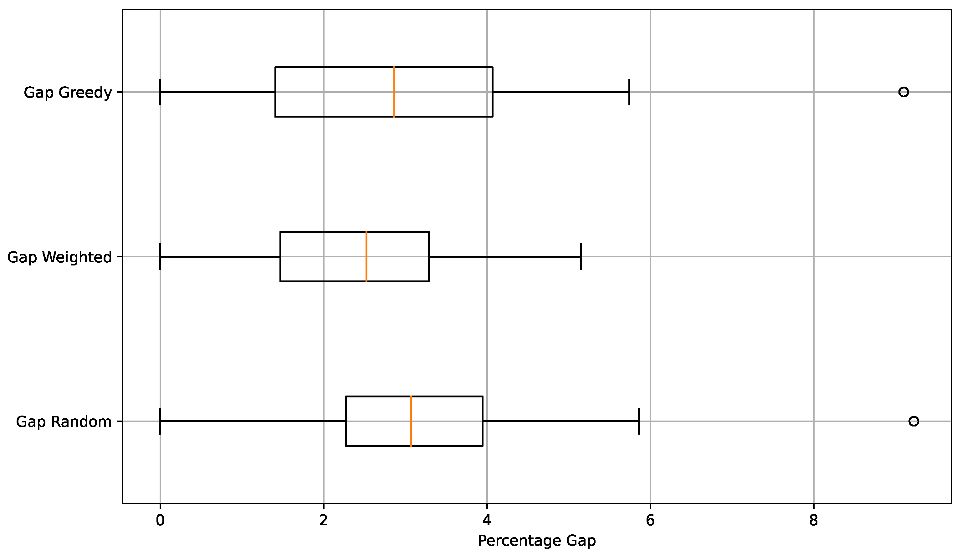
In Figure 3, the % gap of average value, defined in Equation (8), is compared with respect to the best-known value for the different variants developed in this experiment. The comparison is made through box plots. In the figure, it can be observed that visually, the three box plots are similar; however, the median is relatively better for the weighted operator. On the other hand, it is observed that both random and weighted operators have one outlier each. In both cases, it occurred for the same instance, sukp-200-185-0.15-0.85. The dispersion in the case of the greedy operator was greater than that of the other two, even though it is not apparent in the average.

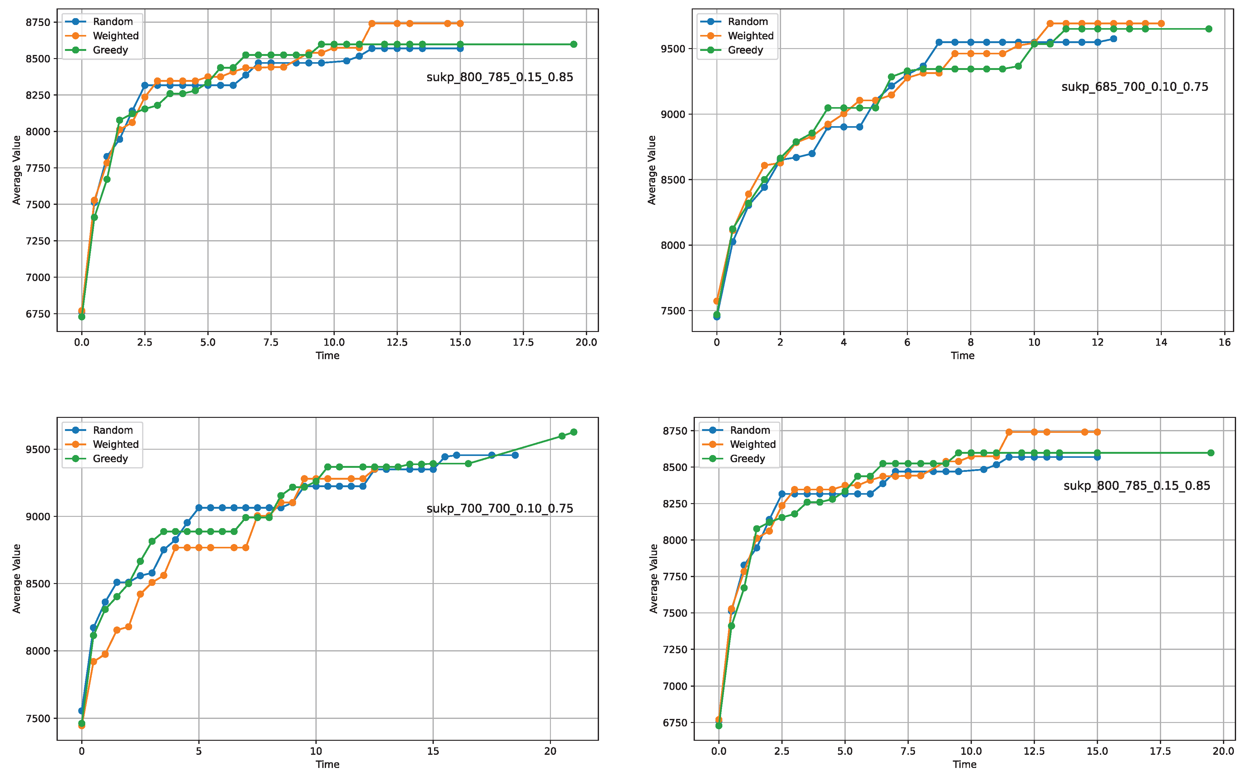
The convergence patterns for four instances are delineated in Figure 4. On initial observation, all plots exhibit analogous trends of convergence, yet certain distinctions arise when delving into the specifics. Notably, the greedy operator demonstrates slower convergence rates in the cases of graphs ’a’ and ’c’ compared to the other two operators. However, this pattern is intriguingly inverted in the context of graph ’d’. Such variations indicate that, on average, the performance disparities among the operators tend to counterbalance across different instances.

$$\%-Gap=100\ast \frac{BestknownValue-AverageValue}{BestknownValue}$$

(8)

Experimental findings derived from large-sized instances of the set-union knapsack problem are presented in

Table 3. Comparison of initialization operators: random, weighted, and greedy for the large-sized instance set.

		Random				Weighted				Greedy
Instances	Best Known	Best Value	Average	Time (s)	Std	Best Value	Average	Time (s)	Std	Best Value	Average	Time (s)	Std
1000_1000_0.10_0.75	9544	8985.00	8429.47	7.15	365.16	9084.00	8428.63	5.41	259.40	9046.00	8347.77	5.75	270.27
1000_1000_0.15_0.85	8474	8129.00	7524.07	7.56	369.28	8165.00	7616.43	8.34	341.37	8079.00	7550.73	9.61	338.77
1000_985_0.10_0.75	9668	8776.00	8165.17	4.39	336.53	9170.00	8318.83	5.46	390.16	8788.00	8221.97	5.15	320.91
1000_985_0.15_0.85	8453	8159.00	7528.70	5.50	379.77	8159.00	7528.70	5.50	379.77	8159.00	7741.67	6.58	351.04
585_600_0.10_0.75	10,393	10,334.00	9932.16	9.26	146.26	10,334.00	9959.27	8.15	146.26	10,233.00	9880.33	8.95	156.26
585_600_0.15_0.85	9256	9256.00	8802.11	6.57	164.13	9256.00	8812.53	6.57	164.13	9256.00	8827.27	7.69	155.69
600_585_0.10_0.75	9914	9741.00	9680.72	3.04	41.50	9741.00	9681.61	3.15	41.50	9914.00	9676.73	4.91	65.38
600_585_0.15_0.85	9357	9357.00	9052.14	10.01	137.27	9357.00	9054.07	9.86	137.27	9258.00	9042.67	7.96	95.32
600_600_0.10_0.75	10524	10,469.00	10,350.58	6.57	101.44	10,490.00	10,384.70	6.70	91.87	10,469.00	10,354.77	6.00	74.25
600_600_0.15_0.85	9062	9024.00	8847.17	5.47	73.51	9024.00	8857.09	6.67	80.37	8976.00	8834.93	5.91	67.09
685_700_0.10_0.75	10,121	9827.00	9420.17	8.16	235.36	9926.00	9548.40	10.38	182.61	9786.00	9472.53	8.89	201.18
685_700_0.15_0.85	9256	8990.00	8699.40	10.20	148.28	9110.00	8779.23	9.04	124.60	9110.00	8727.57	8.12	140.91
700_685_0.10_0.75	9881	9635.00	9397.32	8.69	196.04	9736.00	9452.77	8.07	226.74	9695.00	9410.73	7.39	147.66
700_685_0.15_0.85	9163	9106.00	8811.93	8.24	158.98	9135.00	8790.23	9.75	171.42	9106.00	8718.53	10.97	176.12
700_700_0.10_0.75	9786	9585.00	9138.30	9.88	357.45	9467.00	9171.78	10.02	235.85	9637.00	9307.93	10.76	145.67
700_700_0.15_0.85	9229	8886.00	8582.13	7.68	147.98	8924.00	8602.87	8.70	172.41	9143.00	8664.43	7.13	219.65
785_800_0.10_0.75	9384	9096.00	8640.27	9.71	266.71	9077.00	8603.40	9.95	353.37	9124.00	8627.97	8.71	214.81
785_800_0.15_0.85	8746	8355.00	8062.07	7.87	238.44	8572.00	8159.53	9.64	181.67	8366.00	8095.37	10.11	186.26
800_785_0.10_0.75	9837	9525.00	9091.67	11.18	324.68	9577.00	9060.83	12.39	297.77	9343.00	8955.30	9.54	314.30
800_785_0.15_0.85	9024	8679.00	8456.63	7.12	142.71	8907.00	8555.93	7.13	145.52	8907.00	8498.40	7.31	152.91
800_800_0.10_0.75	9932	9607.00	9309.73	10.26	227.54	9786.00	9372.37	10.36	216.12	9661.00	9413.87	9.43	171.85
800_800_0.15_0.85	9101	8864.00	8389.17	8.97	287.13	8841.00	8395.37	8.11	275.12	8804.00	8381.90	8.17	242.94
885_900_0.10_0.75	9318	9058.00	8656.77	7.97	304.85	9019.00	8596.40	7.31	282.41	9030.00	8653.27	7.73	228.28
885_900_0.15_0.85	8425	8125.00	7669.23	9.88	297.90	8027.00	7568.77	8.21	318.22	8120.00	7620.40	9.08	325.51
900_885_0.10_0.75	9725	9177.00	8859.87	8.70	346.50	9464.00	8953.63	9.16	327.09	9305.00	8861.33	7.85	315.26
900_885_0.15_0.85	8620	8385.00	7814.57	7.69	327.92	8427.00	7902.33	9.38	324.41	8385.00	7872.33	7.71	342.64
900_900_0.10_0.75	9745	9467.00	8989.50	8.50	323.26	9499.00	8870.77	7.41	406.92	9465.00	8949.40	9.28	437.68
900_900_0.15_0.85	8990	8510.00	7747.23	5.13	522.61	8647.00	7908.00	7.73	438.39	8647.00	7888.37	6.44	479.86
985_1000_0.10_0.75	9193	8703.00	8106.17	6.42	323.15	8931.00	8076.70	7.06	436.63	8665.00	8062.87	5.70	327.51
985_1000_0.15_0.85	8528	8143.00	7546.13	6.16	294.45	8143.00	7571.37	5.42	281.91	8134.00	7506.23	5.61	332.20
Average	9354.97	9065.10	8658.00	7.80	252.89	9133.17	8686.06	8.07	247.71	9087.03	8672.25	7.85	233.27
Wilcoxon p-value		0.002	0.01							0.02	0.03

The values highlighted in bold represent the optimal outcomes obtained. It’s important to note that these are only marked when the best result is exclusive to a single algorithm. If there are two algorithms yielding identical optimal values, that instance will not be emphasized.

and further elucidated by the illustrative graphics in Figure 5 and Figure 6. From the data in Table 3, it can be seen that superior results for both average and best value metrics were achieved on average by ’weighted’. Upon detailed inspection of individual instances, it was found that 14 ’best values’ were obtained by the ’weighted’ initialization operator, followed by ’random’ and ’greedy’, each achieving three. In terms of ’average’ values, a similar pattern was seen, with 19 optimal averages being obtained by ’weighted’, followed by ’greedy’ with six, and ’random’ with five. These observations suggest that the final outcome of the optimization process can be influenced by the method used for initializing the solutions. This is further confirmed by significance tests, which indicate a statistically significant difference.

Upon examining the box plots, a favorable trend towards better values for the ’weighted’ initialization operator is also discernible within the interquartile range. The dispersion of results appears more controlled, and the median value also demonstrates superior performance. Furthermore, when analyzing convergence times in conjunction with the graphs, it is observed that there is generally no significant difference among them, with very similar timings being recorded across all three operators. The convergence graphs, likewise, exhibit a comparable pattern.

Based on the findings from the experimental study, it can be concluded that superior performance was exhibited by the weighted initialization operator when compared to the random and greedy operators in solving medium to large-sized instances of the set-union knapsack problem. Although the average convergence times were found to be similar across all three operators, the most optimal solutions were consistently achieved by the weighted operator, along with superior average performance. These assertions were further corroborated by the significance analysis, in which superior performance in terms of best value and average was shown by the weighted operator. However, it must be noted that in certain instances, superior performance was achieved by the random and greedy operators over the weighted operator, indicating that the choice of initialization operator may be contingent upon the unique characteristics of each problem instance.

4.3. Comparisons

This section endeavors to contrast the proposed algorithm with a variety of optimization strategies, particularly focusing on BABC [24], binDE [24], gPSO [14], intAgents [34], and DH-Jaya [26]. The gPSO algorithm commences by creating a randomly populated binary set. By employing crossover and gene selection mechanisms, it generates new particles based on the current, personal, and globally optimal solutions. After the solutions are evaluated and updated accordingly, the algorithm perpetuates iterations until a designated termination criterion is reached. Furthermore, an optional mutation procedure is integrated as needed to preclude premature convergence. The binary artificial bee colony (BABC) is an optimization algorithm that draws inspiration from the foraging practices of honeybees. It incorporates three categories of bees: employed, onlooker, and scout bees. The employed bees actively seek food sources and relay their discoveries to the onlooker bees. Subsequently, the onlookers choose a food source predicated upon its perceived quality. Meanwhile, scout bees traverse uncharted territories in search of superior food sources. The algorithm operates in an iterative manner, continuously refining the food sources until it satisfies a predetermined stopping criterion.

The binary differential evolution (BinDE) algorithm is a population-based optimization strategy. It employs the differential evolution operator to generate novel candidate solutions. The algorithm sustains a population of potential solutions, iteratively updating them by crafting new ones via the differential evolution operator. This operator constructs a new solution by amalgamating two existing solutions with a third, randomly chosen one. Subsequently, the algorithm opts for the superior solution from among the new and existing ones to revamp the population. The algorithm culminates upon reaching a termination criterion, such as attaining a maximum number of iterations or a minimal enhancement in the objective function. The IntAgents algorithm is a swarm-based optimization strategy tailored to solve binary optimization problems. It comprises artificial search agents, each possessing unique cognitive intelligence that enables individual learning within the problem space. While these agents display varied search characteristics, they periodically share information about promising regions. Guided by a central swarm intelligence, these independent agents make use of adaptive information-sharing techniques. These techniques allow the search agents to learn across generations, mitigating the issues of premature convergence and local optima as effectively as possible.

The results are presented in

Table 4. Comparative analysis of MLSCABA and various algorithms in solving SUKP for medium-sized instances.

	Best Known	Best Value						Average Value
Instance		BABC	binDE	gPSO	intAgents	DH-jaya	MLSCABA	BABC	binDE	gPSO	intAgents	DH-jaya	MLSCABA
85_100_0.10_0.75	12045	11,664	11,352	12,045	12,045	12,045	12,045	11,182.7	11,075	11,486.95	11,419.75	11,570.6	11,866.1
85_100_0.15_0.85	12,369	12,369	12,369	12,369	12,369	12,369	12,369	12,081.6	11,875.9	11,994.36	11,885.21	12,318	12,043.5
100_100_0.10_0.75	14,044	13,860	13,814	14,044	14,044	14,044	14,044	13,734.9	13,675.9	13,854.71	13,767.23	13,912.5	13,882.3
100_100_0.15_0.85	13,508	13,508	13,407	13,508	13,508	13,508	13,508	13,352.4	13,212.8	13,347.58	13,003.62	13,439.1	13,174.2
100_85_0.10_0.75	13,283	13,251	13,044	13,283	13,283	13,283	13,283	13028.5	12,991	13,050.53	13,061.02	13,076	13,029.0
100_85_0.15_0.85	12,479	12,238	12,274	12,274	12,274	12,274	12,479	12,155	12,123.9	12,084.82	12,074.84	12,192.5	12,015.0
185_200_0.10_0.75	13,696	13,047	13,024	13,696	13,696	13,696	13,696	12,522.8	12,277.5	13,204.26	13,084.52	13,350.2	13,559.1
185_200_0.15_0.85	11,298	10,602	10,547	11,298	11,298	11,298	11,298	10,150.6	10,085.4	10,801.41	10,780.14	10,828.9	10,923.5
200_185_0.10_0.75	13,521	13,241	13,241	13,405	13,502	13,405	13,502	13,064.4	12,940.7	13,286.56	13,226.28	13,306.6	13,287.4
200_185_0.15_0.85	14,215	13,829	13,671	14,044	14,044	14,215	14,215	13,359.2	13,110	13,492.6	13,441.06	13,660.2	13,234.8
200_200_0.10_0.75	12,522	11,846	11,535	12,522	12,522	12,522	12,522	11,194.3	10,969.4	11,898.73	11,586.26	12,171.6	12,262.8
200_200_0.15_0.85	12,317	11,521	11,469	12,317	11,911	12,187	12,317	10,945	10,717.1	11,584.64	11,288.25	11,746	11,842.5
285_300_0.10_0.75	11,568	11,158	11,152	11,568	11,568	11,568	11,568	10,775.9	10,661.3	11,317.99	11,205.72	11,327.7	11,495.2
285_300_0.15_0.85	11,802	10,528	10,528	11,517	11,517	11,401	11,802	9897.92	9832.32	10,899.2	10,747.33	11,025.9	11,411.3
300_285_0.10_0.75	11,563	10,428	10,420	11,335	11,335	10,934	11,563	9994.76	9899.24	10,669.51	10,576.1	10,703.2	11,346.0
300_285_0.15_0.85	12,607	12,012	11,661	12,245	12,247	12,245	12,402	10,902.9	10,499.4	11,607.1	11,490.26	12,037.5	12,084.5
300_300_0.10_0.75	12,817	12,186	12,304	12,695	12,695	12,695	12,817	11,945.8	11,864.4	12,411.27	12,310.19	12,569.3	12,652.3
300_300_0.15_0.85	11,585	10,382	10,382	11,425	11,425	11,113	11,425	9859.69	9710.37	10,568.41	10,384	10,701.9	11,288.1
385_400_0.10_0.75	10,600	10,085	9883	10,483	10,326	10,414	10,600	9537.5	9314.57	10,013.43	9892.17	10,017	10,357.7
385_400_0.15_0.85	10,506	9456	9352	10,338	10,131	10,302	10,506	9090.03	8846.99	9524.98	9339.67	9565.72	10,175.9
400_385_0.10_0.75	11,484	10,766	10,576	11,484	11,484	11,337	11,484	10,065.2	9681.46	10,915.87	10,734.62	11,062	11,409.6
400_385_0.15_0.85	11,209	9649	9649	10,710	10,710	10,431	11,209	9135.98	9020.87	9864.55	9735	10,017.9	10,725.4
400_400_0.10_0.75	11,665	10,626	10,462	11,531	11,531	11,310	11,665	10,101.1	9975.8	10,958.96	10,756.92	10,914.8	11,501.2
400_400_0.15_0.85	11,325	9541	9388	10,927	10,927	10,915	11,325	9032.95	8768.42	9845.17	9608.07	9969.9	10,976.2
485_500_0.10_0.75	11,321	10,823	10,728	11,094	11,094	10,971	11,260	10,483.4	10,159.4	10,687.62	10,603.53	10,754.8	10,885.8
485_500_0.15_0.85	10,220	9333	9218	10,104	10,104	9715	10,208	9085.57	8919.64	9383.28	9259.36	9467.8	9871.2
500_485_0.10_0.75	11,771	10,784	10,586	11,722	11,722	11,722	11,729	10,452.2	10,363.8	11,184.51	11,111.63	11,269.4	11,504.1
500_485_0.15_0.85	10,238	9090	9191	10,022	10,059	9770	10,059	8857.89	8783.99	9299.56	9165.26	9354.28	9856.2
500_500_0.10_0.75	11,249	10,755	10,546	10,888	10,960	10,960	11,123	10,328.5	10,227.7	10,681.46	10,610.53	10,703.5	10,854.4
500_500_0.15_0.85	10,381	9318	9312	10,194	10,381	10,176	10,381	9180.74	9096.13	9703.62	9578.89	9801.5	9953.8
Average	11,956.9	11,209.4	11,120.1	11,809.8	11,796.4	11,729.0	11,946.8	10,794.1	10,633.2	11,290.8	11,157.9	11,391.0	11,649.0

The values highlighted in bold represent the optimal outcomes obtained. It’s important to note that these are only marked when the best result is exclusive to a single algorithm. If there are two algorithms yielding identical optimal values, that instance will not be emphasized.

. The table indicates that MLSCABA uniquely achieved the optimal values in 19 instances, underscoring its robust performance. Nevertheless, in other situations, at least two algorithms jointly attained the best values, highlighting a competitive landscape. When considering average values, both DH-Jaya and MLSCABA exhibited superior results, with DH-Jaya outperforming in 7 instances and MLSCABA in 23. Notably, while MLSCABA generally yields commendable outcomes, its performance is influenced by the process of solution initialization, indicating that its robustness may be tempered by these initial conditions.

5. Discussion

The findings of this study indicate that the weighted initialization operator tends to outperform the random and greedy operators in most instances of the medium- and large-sized SUKP. This is evident both in terms of the best value obtained and the average value. In particular, the weighted operator achieved the best value in more instances than the other two operators in both datasets. Furthermore, the weighted operator also outperformed the other two operators in terms of the average value in most instances. These results suggest that the weighted operator is more efficient and effective in initializing solutions for this problem.

However, it is important to note that the average execution time was similar among the three operators. This suggests that, although the weighted operator may produce higher-quality solutions, it does not necessarily do so faster than the other operators. Additionally, the convergence plots show that, although all three operators tend to converge to a solution over time, there are some differences in their convergence patterns. For instance, the greedy operator showed a slower convergence rate in some cases, but in other cases, its convergence rate was faster. These differences may be due to the specific characteristics of the problem instances.

In summary, the results suggest that the weighted initialization operator is generally the most effective for the set-union knapsack problem. However, it is also important to consider other factors, such as execution time and the specific characteristics of the problem, when selecting an initialization operator. The results obtained from the comparison of the gPSO, BABC, binDE, intAgents, DH-Jaya, and MLSCABA algorithms in solving the SUKP reveal a variety of strengths and weaknesses in each approach.

The gPSO algorithm, which uses a swarm optimization approach and an iterative process of crossover and gene selection, proved capable of finding optimal solutions in several instances. However, its average performance was surpassed by MLSCABA and DH-Jaya, suggesting it may struggle to maintain consistent performance across multiple iterations. On the other hand, BABC, which draws inspiration from the behavior of bees to search for and improve solutions, achieved the best value in some instances, but its average performance was inferior to that of MLSCABA and DH-Jaya. This may indicate that, although BABC’s approach can be effective in finding optimal solutions, it may not be as effective in maintaining consistent performance across multiple iterations.

The intAgents algorithm, which uses a swarm-based optimization strategy with artificial search agents, achieved the best value in several instances, but its average results were inferior to those of MLSCABA and DH-Jaya. This may indicate that, although intAgents’ approach can be effective in finding optimal solutions, it may struggle to maintain consistent performance across multiple iterations.

DH-Jaya showed solid performance both in terms of the best values and average results. Although it did not achieve the best value in as many instances as MLSCABA, it surpassed MLSCABA in terms of average results in several instances. This suggests that DH-Jaya may be a viable option for this problem, especially in situations where the average quality of the solution is more important than achieving the best possible value. Finally, the proposed algorithm, MLSCABA, achieved the best value in most instances and also showed solid performance in terms of average results. However, its performance may be affected by the initial conditions of the solution, suggesting that the selection of a good initialization operator may be crucial for its performance.

6. Conclusions

In the context of this research, three solution initialization methods were developed and evaluated: random, greedy, and weighted. These methods were integrated and tested in relation to a sine cosine algorithm that uses k-means as a binarization procedure. Tests were conducted with medium- and large-sized instances, and the results show that the solution initialization method significantly impacts the performance of the algorithm.

Specifically, it was observed that the weighted method, which introduces some control over the weight of each item while also incorporating a random component, exhibits superior performance compared to the greedy method. The latter focuses its attention on the quality of items based on a specific heuristic, but does not introduce random elements into the process.

In addition, the weighted method was proven to perform better than the completely random method (random), which does not consider any heuristic for the construction of functions. Regarding convergence times, no significant differences were observed among the methods. However, an improvement in terms of the quality of the solutions obtained was noted, which reiterates the importance of the initialization strategy on the effectiveness of the algorithm.

This study, while concentrating on the set union knapsack problem, unveils initialization methods with potentially broader applicability to a diverse range of combinatorial problems. These might encompass challenges as varied as the traveling salesman problem (TSP), vehicle routing problem (VRP), job shop scheduling problem (JSSP), and quadratic assignment problem (QAP). Each of these problems presents its own unique set of challenges, thus creating a plethora of opportunities for more in-depth examination and investigation in future studies.

Moreover, we believe that there is an opportunity to enhance the solution initialization process further. In this regard, one promising avenue for future research involves the development of adaptive initialization methods. Such methods, with the ability to modulate their behavior based on either the specific characteristics of the problem instance or the algorithm’s progress, could potentially contribute to a more refined, efficient, and effective problem-solving approach.