Article

Observer-Based Fuzzy Control of Uncertain Nonlinear Singular Systems under Multi-Performance Requirements

Department of Marine Engineering, National Taiwan Ocean University, Keelung 202301, Taiwan
*
Author to whom correspondence should be addressed.
Mathematics 2023, 11(12), 2632; https://doi.org/10.3390/math11122632
Submission received: 7 May 2023 / Revised: 28 May 2023 / Accepted: 7 June 2023 / Published: 8 June 2023
(This article belongs to the Special Issue Advanced Methods in Fuzzy Control and Their Applications)

Abstract

:
This paper discusses an observer-based fuzzy control problem for uncertain nonlinear singular systems under Multi-Performance Requirements (MPRs). The approach used in the paper is to model the system using a Takagi–Sugeno (T-S) fuzzy model that can be analyzed using linear control theories. The proposed control scheme is based on the Parallel Distributed Compensation (PDC) approach and Proportional Derivative (PD) control scheme. The goal is to design an observer-based fuzzy controller that achieves stability of the system and also satisfies the Guarantee Cost Control (GCC) constraint while maintaining a desired passive constraint. The stability analysis is performed using Lyapunov theory, and the sufficient conditions are transformed into a Linear Matrix Inequality (LMI) form using a Shur Complement, free-weighting matrix method and Singular Value Decomposition (SVD) techniques. The LMI conditions are then solved using convex optimization algorithms. Finally, the proposed control method is validated using a bio-economic system to demonstrate its effectiveness.

1. Introduction

Singular systems have been of great interest to the field of control theory because they can more accurately represent practical systems with complex dynamics such as bio-economic systems [1], oil catalytic cracking processes [2], electrical circuit systems [3], etc. However, the stability analysis of singular systems is more challenging than those of normal systems. The presence of impulsive behavior is a critical issue that must be addressed before any stability analysis can be performed. To ensure the stability of singular systems, it is necessary to eliminate impulsive behavior. In addition, according to [4], one can find that one approach to achieve this is through matrix decompositions or the use of a controller. In [5,6,7], the researchers investigated various control issues related to linear singular systems, including delay-dependent control, output feedback control and optimal control, respectively. Overall, the study of singular systems and their control is an active area of research in control theory, with many promising results and applications in various practical systems.
Many practical systems exhibit nonlinear characteristics, which makes it challenging to stabilize them using linear control theories. As a result, researchers have extensively investigated control synthesis for nonlinear singular systems. T-S fuzzy models [8,9,10,11,12,13] are an effective approach for describing nonlinear systems. By constructing several linear subsystems using fuzzy sets and IF-THEN rules, the final output of the T-S Fuzzy Singular System (T-SFSS) [14,15,16,17,18,19] can be obtained through membership functions. To stabilize the T-SFSS with linear control theories, a fuzzy controller with the same membership function as the model can be designed based on the PDC concept [13,20]. However, uncertainties are present in practical systems due to modeling errors or component aging. To solve these effects, robust control methods have developed [17,18,19]. Type-2 T-S fuzzy modeling approaches [21,22] have also been constructed to solve the uncertainty problem in membership functions. Moreover, external disturbances caused by external factors can lead to poor control performance, which can make the system unstable. To mitigate the impact of external disturbances, passive theory is used. Passive theory [23,24] involves designing a controller that attenuates the influence of external disturbances.
In recent years, state feedback control methods have been commonly used for analyzing the stability of T-SFSSs. However, in practical systems, it may not be possible to measure the entire state information, which can make it difficult to design a controller. To overcome this challenge, observer theories were investigated in [25,26] to estimate the unmeasurable states. Additionally, research [27,28] has shown that the impulse behaviors in T-SFSSs can be effectively eliminated using derivative state feedback. To address this, the PD control method was proposed in [27,28], which uses the derivative feedback of the PD fuzzy controller to ensure regularity and non-impulsiveness of T-SFSSs. Additionally, the procedure for guaranteeing the regularity and non-impulsiveness using PD fuzzy controllers with derivative feedback is simpler than that of the pure state feedback fuzzy controller. To acquire complete state information of PD fuzzy controllers, an Observer-Based PD (OBPD) fuzzy controller was developed for T-SFSSs in [29,30,31]. Unfortunately, passive control and robust control were not addressed in these studies, which are essential for ensuring the stability of T-SFSSs. Therefore, passive control and robust control are important issues that will be discussed in this paper for determining the stability criterion of T-SFSSs. In addition to stabilization, there have been efforts to assign certain performance criteria when designing controllers. One approach to this is GCC [32,33], which aims to stabilize the system while ensuring an adequate level of performance expressed by a quadratic cost function.
Referring to the above motivations, an OBPD fuzzy control approach is discussed for dealing with uncertain T-SFSSs subject to MPRs. The proposed control scheme employs the PDC concept along with the PD control method. The aim was to ensure the stability of the system while satisfying the GCC constraint under passive constraints. Based on the Lyapunov theory, the sufficient conditions are obtained. These conditions are then transformed into an LMI form using various techniques such as Schur complement, free-weighting matrix and SVD [30]. The LMI conditions can be efficiently solved using convex optimization algorithms [34]. Finally, the effectiveness of the proposed control method was demonstrated by applying it to a nonlinear bio-economic system. The main contributions of this paper can be summarized as follows: (1) Although the PD control method has been applied for the nonlinear singular system in some papers, only a few researchers focused on the observer-based fuzzy control method for T-SFSSs. Based on the T-SFSS, this paper not only developed the fuzzy observer to estimate the unmeasured states, but also proposed a PD fuzzy controller with estimated states to eliminate impulsive behaviors of nonlinear singular systems. Via the OBPD fuzzy controller design method, the MPRs can be combined into the design method to achieve better performances for the nonlinear singular system. (2) For the practical applications, it is expected that the control force can be smaller to achieve the purpose of cost-effectiveness. In this paper, the GCC constraint and passive performance constraint were simultaneously combined into the OBPD fuzzy controller design method. However, the stability analysis will become more difficult and challenging when MPRs are combined. The problem also was efficiently solved by applying mathematical techniques such as SVD and free-weighting matrices. Via the OBPD fuzzy controller design method, the stability of nonlinear singular systems can be achieved with a more cost-effective control effort even under the effect of uncertainty and external disturbances. To the best of our knowledge, the OBPD fuzzy controller design method for uncertain T-SFSSs subject to MPRs constraints has not been developed.
The subsequent sections of this paper are organized as follows. The uncertain T-SFSS with external disturbances and OBPD fuzzy controller are described in Section 2. In Section 3, the stability analysis of the considered system is discussed. In Section 4, an example is used to illustrate the effectiveness of the proposed design method. The conclusion is presented in Section 5.

Notation and Nomenclature

s y m represents the shorthand of + T . n x represents the n x -dimensional vector. h i j and h i represent the shorthand of i = 1 n j = 1 n h i h j and i = 1 n h i , respectively. r a n k ( ) denotes the rank of . denotes the symmetric term in the matrix.

2. System Descriptions and OBPD Control Method

In this section, the T-S fuzzy model is utilized to express the uncertain nonlinear singular system with external disturbance as follows:
Plant Rule i:
If q 1 t is M i 1 and q r t is M i r , then
E x ˙ t = A i + Δ A i t x t + B i + Δ B i t u t D i + Δ D i t w t
z t = C z i x t + J i w t
y t = C y i x t
where q t = q 1 t q 2 t q r t are the premise variables, M i r is the fuzzy set, r is the number of premise variables, i = 1 , 2   ,   m and m is the number of rules, x t n x is the state vector, u t n u is the control input vector, w t n w is the external disturbance vector, y t n y is the measured output vector and z t n z is the output vector. A i n x × n x , B i n x × n u , C y i n y × n x , D i n x × n w , C z i n z × n x and J i n z × n w are constant matrices. E n x × n x is a constant matrix with r a n k ( E ) < n x . Δ A i t n x × n x , Δ B i t n x × n u and Δ D i t n x × n w are the unknown matrices describing uncertainties, which are expressed as Δ A i , Δ B i and Δ D i in the following context and are given as
Δ A i Δ B i Δ D i = H i Δ t W A i W B i W D i
where H i , W A i , W B i and W D i denote the known matrices and Δ t denotes the unknown time-varying function satisfying Δ T t Δ t I .
Hence, the following overall T-S fuzzy model is designed.
E x ˙ t = i = 1 m h i q t A i + Δ A i x t + B i + Δ B i u t + D i + Δ D i w t
z t = i = 1 m h i q t C z i x t + J i w t
y t = i = 1 m h i q t C y i x t
where h i q t = l = 1 r M i l q l t i = 1 m l = 1 r M i l q l t , h i q t 0 , i = 1 m h i q t = 1 and M i l q l t is the grade of the membership of q l t in M i l . For simplification, h i q t h i is defined in the following context.
To overcome the problem with unmeasurable states, the following PD fuzzy observer is constructed.
Observer Rule i:
If q 1 t is M i 1 and… and q r t is M i r , then
E x ^ ˙ t = A i x ^ t + B i u t + L p i y t y ^ t + L d i y ˙ t y ^ ˙ t
y ^ t = C y i x ^ t
where x ^ t n x and y ^ t n y are the estimated state vector and estimated output vector, respectively. The matrices L p i and L d i are the observer gains. Then, the following overall fuzzy observer can be described.
E x ^ ˙ t = i = 1 m h i A i x ^ t + B i u t + L p i y t y ^ t + L d i y ˙ t y ^ ˙ t
y ^ t = i = 1 m h i C y i x ^ t
Based on the PDC concept and PD control method, the OBPD fuzzy controller can be established as follows:
Controller Rule i:
If q 1 t is M i 1 and… and q r t is M i r , then
u t = F p i x ^ t F d i x ^ ˙ t
where F p i and F d i are controller gains. Then, the following overall fuzzy controller can be expressed.
u t = i = 1 m h i F p i x ^ t F d i x ^ ˙ t
Assumption 1 is to ensure the observability and controllability of system (3). Additionally, Assumption 2 assumes the output matrix C can be described by SVD.
Assumption 1. 
If the following equalities are held, system (3) is completely controllable and completely observable.
r a n k s E A i B i = r a n k E B i = n x   a n d   r a n k s E A i C y i = r a n k E C y i = n x
where   s + +  is the open right-half of the complex plane.
Assumption 2. 
([30]). Assume that the output matrix  C y n y × n x  has full row rank, the SVD of matrix  C y  is expressed as
C y = U T V T = U T V 1
where  T = Λ y × y 0 y × x y n y × n x . Λ  is a diagonal matrix with positive diagonal elements.  U n y × n y  and  V n x × n x  are orthogonal matrices.
Remark 1. 
To develop the OBPD fuzzy controller design method in this paper, the SVD technology was applied to solve the problem in the stability analysis. However, the output matrix  C y i  of the T-S fuzzy model (1)–(3) and fuzzy observer (4)–(5) is required to be set as a constant matrix for the SVD technology, that is,  C y 1 = C y 2 = = C y m = C y . Because of this reason, the measured output is considered as the linear case of  y t = C y i x t  for the T-S fuzzy model (3c) and  y ^ t = C y i x ^ t  for the fuzzy observer (5b). Nevertheless, the measured output of the nonlinear system is usually constructed as the linear output in many existing papers [17,18]. Although the setting of constant matrix  C y  will limit the design flexibility fuzzy model and fuzzy controller, the OBPD fuzzy controller design method in this paper is still sufficiently applicable for the control of uncertain nonlinear singular systems.
By defining the estimation error function e t = x t x ^ t and applying Equations (3a) and (5a), one can derive the following relationship equation.
E e ˙ t = E x ˙ t E x ^ ˙ t = i = 1 m j = 1 m h i h j Δ A i Δ B i F p j x t + A i + Δ B i F p j L p i C y e t Δ B i F d j x ˙ t + Δ B i F d j L d i C y e ˙ t + D i + Δ D i w t
From Equations (3a) and (8), the augmented system can be obtained as follows:
E 0 0 E x ˙ t e ˙ t = i = 1 m j = 1 m h i h j A i + Δ A i B i F p j Δ B i F p j B i F p j + Δ B i F p j Δ A i Δ B i F p j A i + Δ B i F p j L p i C y x t e t + B i F d j Δ B i F d j B i F d j + Δ B i F d j Δ B i F d j Δ B i F d j L d i C y x ˙ t e ˙ t + D i + Δ D i D i + Δ D i w t }
By arranging Equation (9), the equation can be further obtained as follows:
E ˜ R i j h i j x ˜ ˙ t = A ˜ R i j h i j x ˜ t + D ˜ i h i w t
where x ˜ t = x T t e T t T , E ˜ R i j = E R i j + H ˜ i Δ t W ˜ B D i j , E R i j = E + B i F d j B i F d j 0 E + L d i C y , H ˜ i = H i H i , W ˜ B D i j = W B i F d j W B i F d j , A ˜ R i j = A R i j + H ˜ i Δ t W ˜ A i + W ˜ B P i j , A R i j = A i B i F p j B i F p j 0 A i L p i C y , W ˜ A i = W A i 0 , W ˜ B P i j = W B i F p j W B i F p j , D ˜ i = D R i + H ˜ i Δ t W D i and D R i = D i D i .
According to Assumption 1, E R i j is turned invertible by gains F d j and L d i . The following equation can thus be obtained from Equation (10).
x ˜ ˙ t = E ˜ R i j 1 h i j A ˜ R i j h i j x ˜ t + D ˜ i h i w t
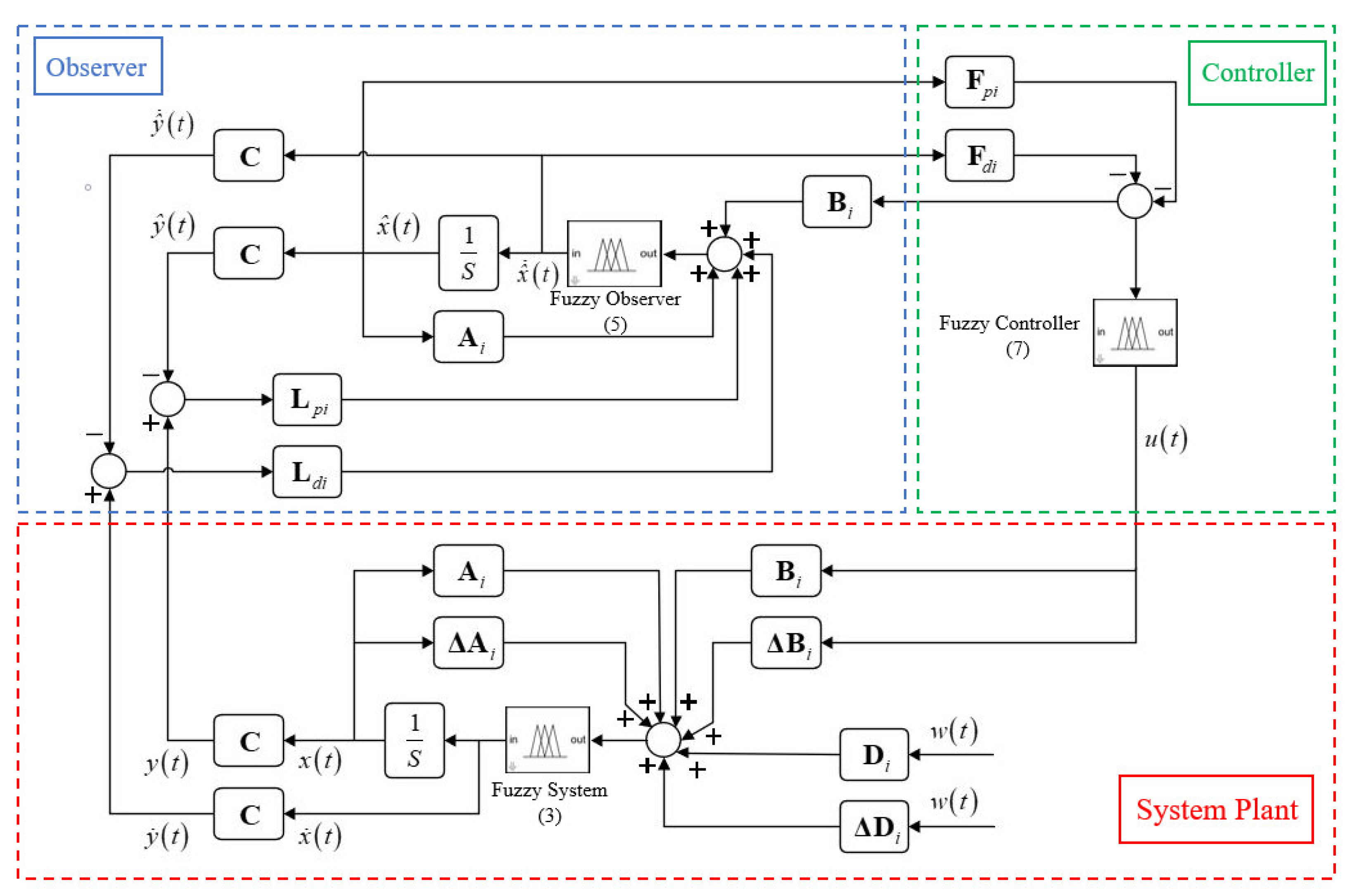
The following figure is provided to illustrate the relationship between the module of all components in a clear and comprehensive manner. Firstly, the T-SFSS (3) in the System Plant part is established for the representation of an uncertain nonlinear singular system under the effect of external disturbances. Then, the fuzzy observer (4) is designed with the same premise part of the fuzzy model and the overall fuzzy observer (5) in the Observer part is developed to estimate the unmeasured states of the T-SSFSS (3). Thus, the estimated states x ^ t and derivative of states x ^ ˙ t obtained by the fuzzy observer (5) can be applied as the feedback signal for the fuzzy controller (7), which is presented in the Controller Part. Finally, the control input u t provided by the fuzzy controller (7) is designed by the OBPD fuzzy controller design method in the next section. Additionally, the control input can be applied to guarantee the stability and MPRs of the nonlinear singular system under the effect of uncertainty and external disturbance (Figure 1).
Some useful definitions and lemmas are provided next before the stability conditions is derived.
Definition 1. 
([24]). If the following inequality is held given   S 1 S 2 0  and  S 3 , then the system is passive with the external disturbance  w t  and output  z t  for all terminal time  t p > 0 .
2 0 t p z T t S 1 w t d t > 0 t p z T t S 2 z t d t + 0 t p w T t S 3 w t d t
The performance cost function associated with system (3) is defined as follows:
J = 0 x T t N 1 x t + u T t N 2 u t d t
where  N 1  and  N 2  are positive definite symmetric matrices with approximate dimensions.
The following definition of GCC for system (3) is defined.
Definition 2. 
([32]). If there is a controller (7) and a positive scalar  J 0  such that system (3a) is asymptotically stable, and the value of the cost function (13) satisfies  J J 0 , then  J 0 is considered to be a guaranteed cost.
Lemma 1. 
([30]). Given real appropriate dimension matrices  H W  and  Δ ( t )  with  Δ T ( t ) Δ ( t ) I  and a scalar  ε > 0 , one can find the result as follows:
s y m H Δ t W ε H H T + ε 1 W T W

3. Main Results

The main object of this paper was to discuss the stability criterion for system (11). Additionally, the theorem in this paper are given as follows.
Theorem 1. 
Giving the matrices  S 1 S 2 0  and  S 3 , system (11) is asymptotically stable and passive if there is the matrices  X ¯ = X ¯ T > 0 K 1 j K 2 j Y 1 i Y 2 i R ¯ 1  and  R ¯ 2 , and a scalar  ε such that the following sufficient condition is held.
s y m R ¯ 1 0 Θ 13 0 Θ 15 0 Θ 17 X ¯ C z i T S 2 s y m R ¯ 1 K 1 j T B i T Θ 24 0 0 K 1 j T W B i T 0 Θ 33 B i K 2 j D i ε H i K 2 j T W B i T 0 Θ 44 D i ε H i K 1 j T W B i T 0 Θ 55 0 W D i T 0 ε I 0 0 ε I 0 I < 0 f o r   i , j   =   1 , 2 , ... , m
where  Θ 13 = R ¯ 2 X ¯ A i T + R ¯ 1 T E + K 1 j T B i T Θ 15 = X ¯ C z i T S 2 J i X ¯ C z i T S 1 Θ 17 = X ¯ W A i T + K 1 j T W B i T Θ 24 = R ¯ 2 X ¯ A i T + R ¯ 1 T E + C T Y 1 i T Θ 33 = s y m E R ¯ 2 + B i K 2 j Θ 44 = s y m E R ¯ 2 + Y 2 i C Θ 55 = J i T S 2 J i + S 3 J i T S 1 S 1 T J i K 1 j T = X ¯ F p j T + R ¯ 1 T F d j T K 2 j = F d j R ¯ 2 Y 1 i T = X ^ L p i T + R ^ 1 T L d i T Y 2 i = L d i R ^ 2 R ¯ 1 T = V R 1 T V T = X ¯ Q 1 Q 2 1 R ¯ 2 T = V R 2 T V T = Q 2 1  and  X ¯ = V X V T = P 1 .
Proof. 
Choose the following Lyapunov function:
V x ˜ t = x ˜ T t P ˜ x ˜ t
The following equation can be obtained according to Equation (16) with the free-weighting matrices Q ˜ 1 and Q ˜ 2 .
V ˙ x ˜ t = 2 x ˜ ˙ T t P ˜ x ˜ t + 2 x ˜ T t Q ˜ 1 + x ˜ ˙ T t Q ˜ 2 × E ˜ R i j h i j x ˜ ˙ t + A ˜ R i j h i j x ˜ t + D ˜ i h i w t
where P ˜ = P 0 P , Q ˜ 1 = Q 1 0 Q 1 and Q ˜ 2 = Q 2 0 Q 2 .
Then, the Lyapunov function (17) can be rewritten as follows:
V ˙ x ¯ t x ¯ T t Ψ i j x ¯ t
where x ¯ T t = x ˜ T t x ˜ ˙ T t w T t and Ψ i j h i j = s y m Q ˜ 1 A ˜ R i j h i j P ˜ Q ˜ 1 E ˜ R i j h i j + A ˜ R i j T h i j Q ˜ 2 T Q ˜ 1 D ˜ R i h i s y m Q ˜ 2 E ˜ R i j h i j Q ˜ 2 D ˜ R i h i 0 .
Based on Definition 1, the following performance function is defined for the case of w t 0 .
Γ z , w , t = 0 t p z T t S 2 z t + w T t S 3 w t 2 z T t S 1 w t d t = 0 t p z T t S 2 z t + w T t S 3 w t 2 z T t S 1 w t + V ˙ x ¯ t d t V x ¯ t p 0 t p z T t S 2 z t + w T t S 3 w t 2 z T t S 1 w t + V ˙ x ¯ t d t = 0 t p G z , w , t d t
where
G z , w , t = z T t S 2 z t + w T t S 3 w t 2 z T t S 1 w t + V ˙ x ˜ t
Substituting Equations (3b) and (18) into Equation (20), one can obtain:
G z , w , t = x ¯ T t Ψ ˜ i j h i j x ¯ t
where
Ψ ˜ i j h i j = i = 1 m j = 1 m h i h j s y m Q ˜ 1 A ˜ R i j + C ˜ z i T S 2 C ˜ z i P Q ˜ 1 E ˜ R i j + A ˜ R i j T Q ˜ 2 T Q ˜ 1 D ˜ R i + C ˜ z i T S 2 J i C ˜ z i T S 1 s y m Q ˜ 2 E ˜ R i j Q ˜ 2 D ˜ R i Θ 55
Pre- and post-multiplying X ˜ R ˜ 1 T 0 0 R ˜ 2 T 0 0 0 I and its transpose matrix on Ψ ˜ i j , the following inequality is inferred:
s y m R ˜ 1 + X ˜ C ˜ z i T S 2 C ˜ z i X ˜ R ˜ 2 X ˜ A ˜ R i j T + R ˜ 1 T E ˜ R i j T X ˜ C ˜ z i T S 2 J i X ˜ C ˜ z i T S 1 s y m E ˜ R i j R ˜ 2 D ˜ R i Θ 55 < 0
where X ˜ = X ¯ 0 X ¯ , R ˜ 1 = R ¯ 1 0 R ¯ 1 and R ˜ 2 = R ¯ 2 0 R ¯ 2
Applying Lemma 1, the uncertain matrices of Equation (22) can be transferred as follows:
s y m H ¯ i Δ t W ¯ i j ε H ¯ i H ¯ i T + ε 1 W ¯ i j T W ¯ i j
where H ¯ i T = 0 H ˜ i T 0 and W ¯ i j = W ˜ B D i j R ˜ 1 W ˜ A i X ˜ W ˜ B P i j X ˜ W ˜ B D i j R ˜ 2 W ˜ D i . According to Equations (22) and (23), the inequality can be obtained as follows:
s y m R ˜ 1 + X ˜ C ˜ z i T S 2 C ˜ z i X ˜ R ˜ 2 X ˜ A R i j T + R ˜ 1 T E R i j T X ˜ C ˜ z i T S 2 J i X ˜ C ˜ z i T S 1 s y m E R i j R ˜ 2 D ˜ R i Θ 55 + ε H ¯ i H ¯ i T + ε 1 W ¯ i j T W ¯ i j < 0
The following inequality can be derived by applying a Schur complement to Equation (24):
s y m R ¯ 1 0 Θ 13 0 Θ 15 0 Θ 17 X ¯ C z i T S 2 s y m R ¯ 1 K 1 j T B i T Θ ¯ 24 0 0 K 1 j T W B i T 0 Θ 33 B i K 2 j D i ε H i K 2 j T W B i T 0 Θ ¯ 44 D i ε H i K 1 j T W B i T 0 Θ 55 0 W D i T 0 ε I 0 0 ε I 0 I < 0
where Θ ¯ 24 = R ¯ 2 X ¯ A i T + R ¯ 1 T E + X ¯ C T L p i T + R ¯ 1 T C T L d i T and Θ ¯ 44 = s y m E R ¯ 2 + L d i C R ¯ 2 .
According to Assumption 2, the following inequality can be inferred from Equation (25) by defining Y 1 i T = X ^ L p i T + R ^ 1 T L d i T and Y 2 i = L d i R ^ 2 :
s y m R ¯ 1 0 Θ 13 0 Θ 15 0 Θ 17 X C z i T S 2 s y m R ¯ 1 K 1 j T B i T Θ 24 0 0 K 1 j T W B i T 0 Θ 33 B i K 2 j D i ε H i K 2 j T W B i T 0 Θ 44 D i ε H i K 1 j T W B i T 0 Θ 55 0 W D i T 0 ε I 0 0 ε I 0 I < 0
Then, one can find that Equation (26) is equivalent to condition (15). Furthermore, if Equation (26) is held, it implies Ψ ˜ i j h i j < 0 such that G z , w , t < 0 is obtained from Equation (21). Therefore, the passive performance of system (11) is realized when condition (15) is established. To analyze the stability of system (11), the following inequality can be derived from Equation (20) and by assuming w t = 0 :
V ˙ x ¯ t < x T t C z i T S 2 C z i x t
Since S 2 0 , V ˙ x ¯ t < 0 can be inferred by (27). Therefore, system (11) is asymptotically stable and passive if condition (15) is held. The proof of Theorem 1 is completed. □
Remark 2. 
In practical applications, the dynamic states and derivative states of a system are not always possible to be directly measured. This derives a challenge for the PD control scheme, which typically assumes that all states are measurable [7,28]. To address the problem, the concept of observer-based control [29,30,31] has been applied as a viable solution in this paper to estimate the derivative states of the feedback signals for the PD controller. Based on the T-SFSS (3), fuzzy observer (5) and PD fuzzy controller (7), an OBPD fuzzy controller design method was proposed in Theorem 1 based on a closed-loop system (11). Combining the passive constraint (12) with the Lyapunov stability theory, the sufficient condition (15) was successfully derived by applying the free-weighting matrix (17) and the SVD technology in Assumption 1. Via satisfying the condition (15), the stability and passive performance can be simultaneously guaranteed for nonlinear singular systems with uncertainty and disturbance.
Theorem 2. 
Given the matrices  S 1 S 2 0  and  S 3 , if there exist the matrices  X ¯ = X ¯ T > 0 , K 1 j , K 2 j , Y 1 i , Y 2 i , R ¯ 1 , R ¯ 2 , and scalars  γ > 0  and  ε  such that the following stability conditions and condition (15) are held, then, the OBPD fuzzy controller (7) is considered to be the GCC for system (11) and also satisfies the passive performance constraint.
s y m R ¯ 1 0 Θ 13 0 K 1 j T X ¯ 0 Θ 17 s y m R ¯ 1 K 1 j T B i T Θ 24 K 1 j T 0 0 K 1 j T W B i T Θ 33 B i K 2 j K 2 j T 0 ε H i K 2 j T W B i T Θ 44 K 2 j T 0 ε H i K 1 j T W B i T N ˜ 2 0 0 0 N ˜ 1 0 0 ε I 0 ε I < 0 f o r   i , j   =   1 , 2 , ... , m
γ x T 0 X ¯ < 0
where  N ˜ 1 = N 1 1  and  N ˜ 2 = N 2 1 .
Proof. 
Applying the same construction of Lyapunov function (16) for V ˙ c x ˜ t , the following equation is also obtained with the free-weighting matrices Q ˜ 1 and Q ˜ 2 :
V ˙ c x ˜ t = 2 x ˜ ˙ T t P ˜ x ˜ t + 2 x ˜ T t Q ˜ 1 + x ˜ ˙ T t Q ˜ 2 × E ˜ R i j h i j x ˜ ˙ t + A ˜ R i j h i j x ˜ t
Similar to Theorem 1, the following inequality can be inferred:
V ˙ c x t x T t Ψ i j h i j x t
where x T t = x ˜ T t x ˜ ˙ T t and Ψ i j h i j = s y m Q ˜ 1 A ˜ R i j h i j P ˜ Q ˜ 1 E ˜ R i j h i j + A ˜ R i j T h i j Q ˜ 2 T s y m Q ˜ 2 E ˜ R i j h i j .
Based on Equation (30) and the cost function defined by Equation (13), the inequality can be given as follows:
J = 0 t p x T t N 1 x t + u T t N 2 u t d t = 0 t p x T t N 1 x t + u T t N 2 u t + V ˙ c x t d t V c x t p 0 t p x T t N 1 x t + u T t N 2 u t + V ˙ c x t d t = 0 t p x T t Ξ i j h i j x t d t
where Ξ i j h i j = Ψ i j h i j + Ω ¯ h j , Ω ¯ = Ω 1 Ω 2 Ω 3 , Ω 1 = N 1 + F p j T N 2 F p j F p j T N 2 F p j F p j T N 2 F p j F p j T N 2 F p j , Ω 2 = F p j T N 2 F d j F p j T N 2 F d j F p j T N 2 F d j F p j T N 2 F d j and Ω 3 = F d j T N 2 F d j F d j T N 2 F d j F d j T N 2 F d j F d j T N 2 F d j .
Pre- and post-multiplying X ˜ R ˜ 1 T 0 R ˜ 2 T and its transpose matrix on Ξ i j , the following inequality can be inferred:
s y m R ˜ 1 + X ^ N ˜ 1 X ^ R ˜ 2 X ˜ A ˜ R i j T + R ˜ 1 T E ˜ R i j T s y m E ˜ R i j R ˜ 2 + K ˜ j T N ˜ 2 K ˜ j < 0
where X ^ = X ¯ 0 0 and K ˜ j = K 1 j K 1 j K 2 j K 2 j .
Based on Lemma 1, the uncertain matrices of Equation (32) can be converted as follows:
s y m H ^ i Δ t W ^ i j ε H ^ i H ^ i T + ε 1 W ^ i j T W ^ i j
where H ^ i T = 0 H ˜ i T and W ^ i j = W ˜ B D i j R ˜ 1 W ˜ A i X ˜ W ˜ B P i j X ˜ W ˜ B D i j R ˜ 2 . According to Equation (33) and applying a Schur complement to Equation (32), the inequality can be obtained as follows:
s y m R ¯ 1 0 Θ 13 0 K 1 j T X 0 Θ 17 s y m R ¯ 1 K 1 j T B i T Θ 24 K 1 j T 0 0 K 1 j T W B i T Θ 33 B i K 2 j K 2 j T 0 ε H i K 2 j T W B i T Θ 44 K 2 j T 0 ε H i K 1 j T W B i T N ˜ 2 0 0 0 N ˜ 1 0 0 ε I 0 ε I < 0
Obviously, Equation (34) is equivalent to the condition (28a), which implies Ξ i j h i j < 0 from Equation (31). That is, if the condition (28a) is held, the stability of system (11) with external disturbances can be ensured with the upper bound of the cost function (13). Moreover, because Ξ i j h i j < 0 , it further indicates that the following inequality is held.
x T t N 1 x t + u T t N 2 u t + V ˙ c x t < 0
Integrating Equation (35) from 0 to t p leads to:
J < V c x 0 V c x t p
If system (11) is stable, V c x t p = 0 . Then, the cost function is bounded by V c x 0 and the following inequality is inferred:
J < x T 0 P x 0
Because x ^ T t = 0 for t ,   0 , the estimation error function e t = x t is inferred. Additionally, the following inequality is obtained by replacing x in V c x 0 :
x T 0 P x 0 = x T 0 P x T 0 = J 0
Noticed that J < J 0 is derived from Equations (37) and (38). Additionally, one can easily find that the constraints of Definition 2 are satisfied if condition (28b) is held. Moreover, J 0 is the upper bound of the GCC constraint and the following relation is obtained by setting a scalar:
x T 0 P x T 0 < γ
By using a Shur complement, the following inequality can be rewritten from Equation (39):
γ x T 0 X ¯ < 0
Obviously, Equation (40) is equivalent to Equation (28b). If condition (28b) is satisfied, it implies that the GCC constraint for system (11) can be achieved. Additionally, system (11) satisfies the GCC and passivity constraint when the conditions of Theorem 2 are held. The proof of Theorem 2 is completed. □
Remark 3. 
Extending the OBPD fuzzy controller design method of Theorem 1, the GGC constraint and passive performance constraint are combined into the design method in Theorem 2 to achieve the MPRs for a nonlinear singular system. However, the stability analysis process will become more complex and challenging. In Theorem 2, this drawback was also overcome by applying free-weighting matrix (29) and the SVD technology in Assumption 1. For most practical applications, it is expected that the control force can be designed as small as possible to efficiently reduce the control cost. Via satisfying the sufficient conditions (15), (28a) and (28b), the stability and passive performance can be achieved with a more cost-effective control force for an uncertain nonlinear singular system. Additionally, the GGC constraint which limits the control input will increase the conservativeness of the stability process. In Theorem, the application of free-weighting matrix (29) can also be provided as a tool to obtain more relax stability analysis results.

4. Numerical Examples

The effectiveness of the proposed design method is illustrated in this section using a nonlinear bio-economic system that was studied in [1,31]. Firstly, the nonlinear bio-economic system is presented as follows.
Θ ˙ 1 t = ζ Θ 2 t r 1 Θ 1 t α Θ 1 t η Θ 1 2 t D t Θ 1 t + w t Θ ˙ 2 t = α Θ 1 t r 2 Θ 2 t 0 = D t ρ Θ 1 t c m + u t
where Θ 1 t and Θ 2 t represent the population density of juvenile species and adult species, respectively.   D t represents the harvest effort on the immature population and u t represents the policy for adjusting the tax. ρ represents the price constant per individual population, c represents the cost coefficient and m represents the economic interest of harvesting. The more detailed meaning of the parameters of Equation (41) can be found in [1].
To protect resources and promote economic development, the government implements the adjustment on tax to increase or decrease the cost for harvesting so that the bio-economy system can achieve sustainable development. Referring to [1], the operating points were chosen as x 1 t d , d and d = 10 . The other system coefficients were chosen as ζ = 0.15 , r 1 = 0.2 , r 2 = 0.1 , α = 0.05 , η = 0.001 , ρ = 1 and c = 40 . Additionally, the nonlinear model (41) can be rewritten as the following form by the setting x 1 t = Θ 1 t c ρ , x 2 t = Θ 2 t α c ρ r 2 and x 3 t = D t ζ α ρ α ρ r 2 ρ r 1 r 2 η c r 2 ρ r 2 :
x ˙ 1 t = 0.79 x 1 t + 0.15 x 2 t 40 x 3 t 0.001 x 1 2 t x 1 t x 3 t + w t x ˙ 2 t = 0.5 x 1 t 0.1 x 2 t 0 = 0.01 x 1 t + x 1 t x 3 t m + u t
In addition, we added uncertainty terms to represent modeling errors for simulating the real operating conditions. With these considerations, the corresponding T-S fuzzy model can be expressed as follows:
E x ˙ t = i = 1 2 h i x t A i + Δ A i x t + B i + Δ B i u t + D i + Δ D i w t z t = i = 1 2 h i x t C z i x t + J i w t y t = C y x t
where i = 1 , 2 , E = 1 0 0 0 1 0 0 0 0 , A 1 = 0.78 0.15 30 0.5 0.1 0 0.01 0 10 , A 2 = 0.8 0.15 50 0.5 0.1 0 0.01 0 10 , B i = 0 0 1 , C y = 1 1 0 0 0 1 , C z 1 = C z 2 = 0 0 1 , D i = 1 0 0 , J 1 = J 2 = 1 , Δ A 1 = 0.002 0 0.005 0 0 0 0 0 0 , Δ A 2 = 0.006 0 0.015 0 0 0 0 0 0 , Δ B 1 = 0.001 0 0 , Δ B 2 = 0.003 0 0 , Δ D 1 = 0.002 0 0 and Δ D 2 = 0.003 0 0 
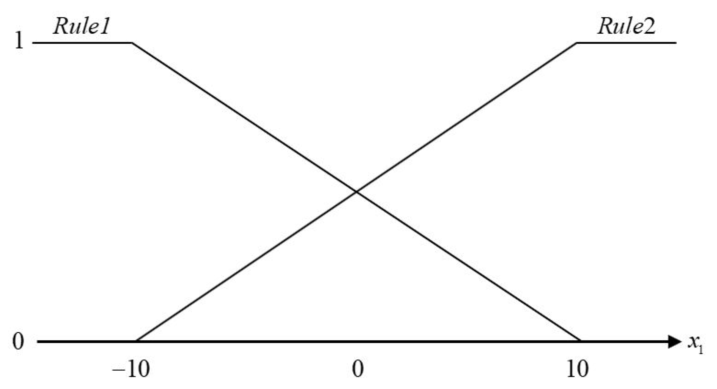
. The membership functions are h 1 x t = 1 2 1 x 1 t 10 and h 2 x t = 1 h 1 x t , which are presented in Figure 2. Moreover, the uncertain parameters are assumed to be as follows from Equation (2):
H 1 = 0.01 0 0 , H 2 = 0.03 0 0 , W A i T = 0.2 0 0.05 , W B 1 = 0.1 , W B 2 = 0.1 , W D 1 = 0.2 , W D 2 = 0.1 and Δ t = s i n t .
Based on Assumption 1, the following matrices U , T and V are obtained by compositing C :
U = 1 0 0 1 ,   T = 1.4142 0 0 1 ,   V = 0.7071 0 0.7071 0.7071 0 0.7071 0 1 0
By setting a scalar γ = 18 and the matrices S 1 = 1 , S 2 = 0.8 and S 3 = 0.8 , the following gains and positive definite matrix can be directly calculated using the convex optimization algorithm:
F d 1 = 3.3984 3.4055 7.0377 ,   F d 2 = 3.4548 3.4505 7.1535 ,   F p 1 = 10 3 × 0.0742 0.0742 1.6105 ,   F p 2 = 10 3 × 0.0754 0.0754 1.6357 ,   L d 1 = 0.9317 1.3680 0.6945 0.8075 43.0746 89.2488 ,   L d 2 = 0.2276 1.0270 0.4160 0.2264 43.0744 89.2098 ,   L p 1 = 10 4 × 0.0022 0.0323 0.0011 0.0228 0.1912 2.0441 ,   L p 2 = 10 4 × 0.0031 0.0246 0.0002 0.0095 0.1910 2.0414 and   P = 0.5266 0.3533 0.5521 0.3533 0.5266 0.5521 0.5521 0.5521 11.6272
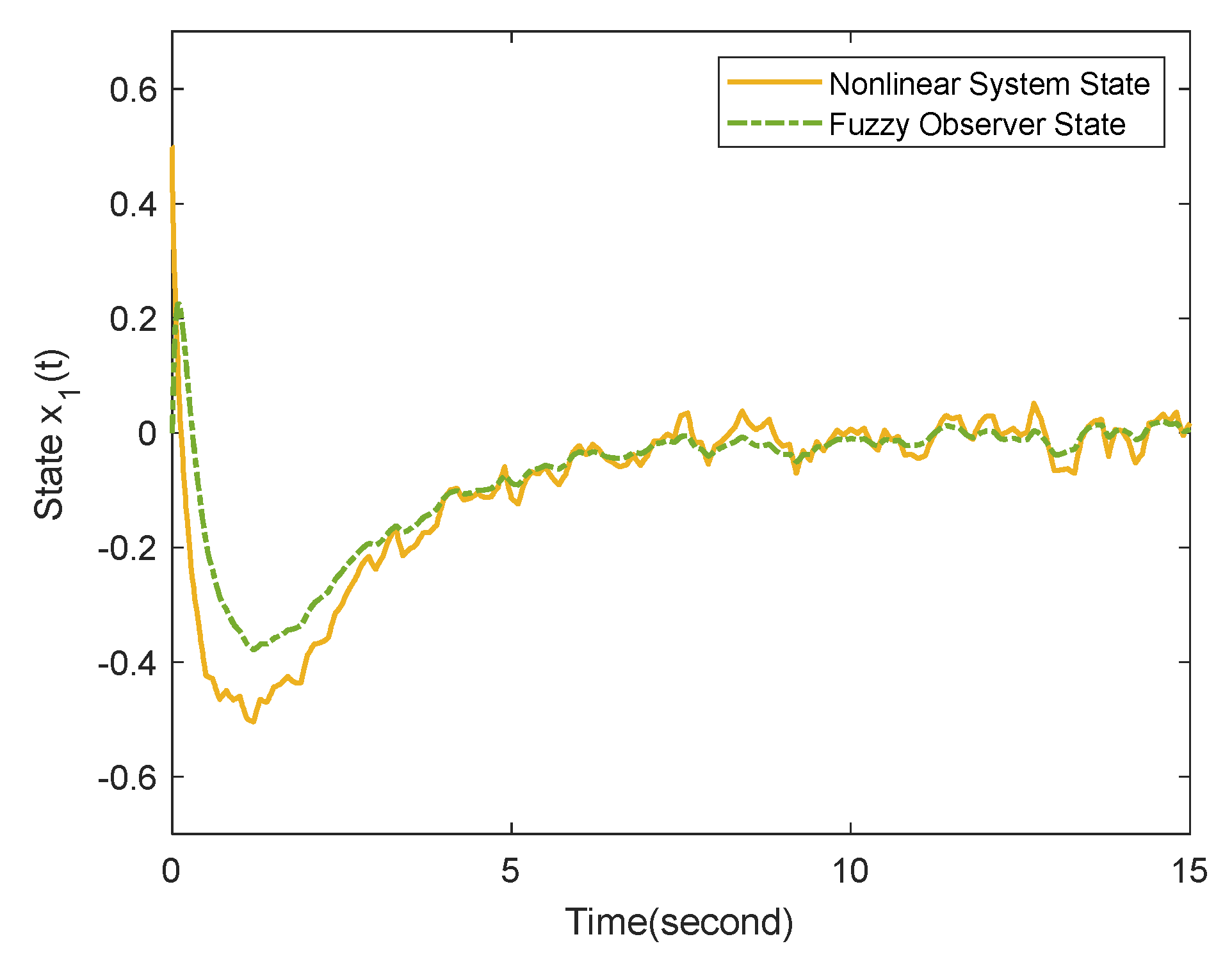
Via the gains presented in Equation (44), the proposed OBPD controller (7) can be designed with the observed states of a fuzzy observer (5) to control the nonlinear bio-economic system. Thus, the state responses of system (42) are depicted in Figure 3, Figure 4 and Figure 5 with the initial conditions x 0 = 0.5 1 0.3 T and x ^ 0 = 0 0 0 T , respectively.
Based on the simulation results in Figure 3, Figure 4 and Figure 5, the passive performance can also be verified as follows. Firstly, the following inequality can be obtained from the passive performance constraint (12) in Definition 1 with the setting of S 1 = 1 , S 2 = 0.8 and S 3 = 0.8 in this simulation:
2 0 t p z T t w t d t 0 t p z T t z t d t + 0 t p w T t w t d t > 0.8
From the inequality (45), one can know that if the value obtained with output z t and external disturbance w t is larger than the threshold value 0.8, the passive performance can be guaranteed for the nonlinear bio-economic system. According to the setting of C z 1 , C z 2 , J 1 , J 2 and C y for the T-S fuzzy model (43), the value based on the term of the right-hand side of Equation (43) was obtained via the simulation results.
2 0 t p z T t w t d t 0 t p z T t z t d t + 0 t p w T t w t d t = 1.248
Obviously, comparing the value of Equation (46) with the threshold value 0.8 in inequality (45), one can find that the passive performance constraint in Definition 1 is satisfied. Therefore, the effect of external disturbance can be effectively attenuated. From the responses in Figure 3, Figure 4 and Figure 5, it becomes evident that the stability of nonlinear bio-economic system was achieved by applying the proposed OBPD fuzzy controller (7) even under the effects of external disturbance and uncertainty. Additionally, it was also seen that the states of the nonlinear system (41) were successfully estimated by the designed fuzzy observer.
Referring to [1,31], the convergence of system states implies that all the states can be controlled to the positive equilibriums for Θ 1 t , Θ 2 t and D t . This also means the juvenile species, the adult species and the harvest effort on the immature population must reach a balance so that the population of the species can be protected from endangerment. Moreover, the proposed OBPD fuzzy controller design method can be provided as a good choice for the government policy to adjust taxes and regulate the cost of harvesting.
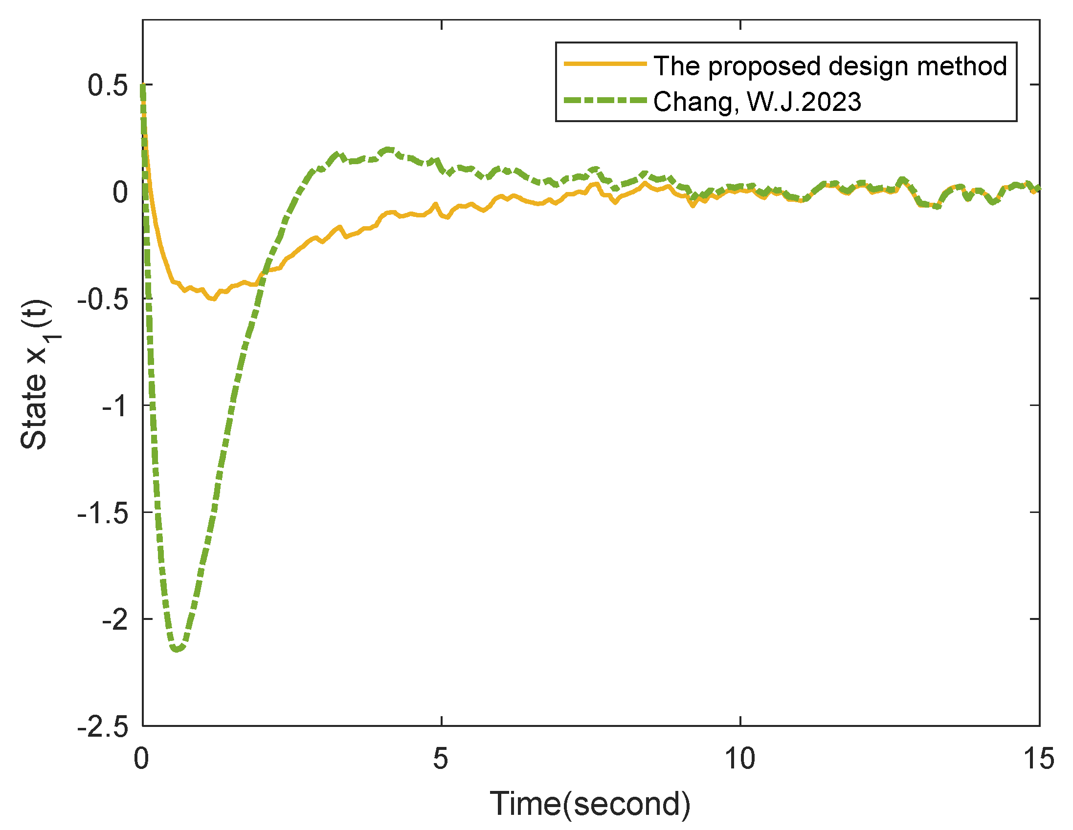
To demonstrate the effectiveness of the proposed OBPD fuzzy control method in the control of nonlinear singular systems, the simulation results comparing the proposed method with the design method in [31] are presented below. Applying the fuzzy control method in [31], the following gains of fuzzy controller and fuzzy observer can be obtained based on the T-SFSS (43):
F d 1 = 10 3 × 0.1132 0.1132 3.5742 , F d 2 = 10 3 × 0.1130 0.1129 3.5687 ,   F p 1 = 10 3 × 0.1691 0.1692 5.3354 ,   F p 2 = 10 3 × 0.1690 0.1689 5.3423 ,   L d 1 = 10 3 × 0.0684 2.1479 0.0869 2.7487 0.1457 4.6306 ,   L d 2 = 10 3 × 0.1300 4.0937 0.1231 3.8890 0.1461 4.6628 ,   L p 1 = 10 3 × 0.0670 2.1076 0.0921 2.8635 0.2965 9.3773   and   L p 2 = 10 3 × 0.1310 4.1506 0.1190 3.7140 0.2969 9.4409
Via selecting the same initial condition x 0 = 0.5 1 0.3 T and x ^ 0 = 0 0 0 T , the state responses of the nonlinear system (41) are presented in Figure 6, Figure 7, Figure 8 and Figure 9 applying the OBPD fuzzy controller (7) and the fuzzy observer (5).
It is worth noting that, although the robust OBPD fuzzy controller subject to passive constraint has also been developed in [31], the GCC performance requirement was considered in this research. However, the stability analysis will become more difficult and challenging if the multi-performance constraints are simultaneously considered in the fuzzy controller design method. Through application of some efficient mathematical techniques, this problem was efficiently solved by the proposed design method. Therefore, the designed fuzzy controller (15) with the gains (44) can achieve stability under the effect of uncertainty and external disturbance by using the smaller control force. From the responses in Figure 9, it is obvious that the control input of the proposed OBPD fuzzy controller design method was smaller than the design method in [31]. On top of that, one can find that the small overshoot of state responses presented in Figure 6, Figure 7 and Figure 8 were obtained by the proposed OBPD fuzzy controller. Additionally, the settling time of all state responses obtained with both design methods was almost the same. Therefore, it can be concluded that the proposed OBPD fuzzy controller design method can obtain better state responses with a more cost-effective control force even when affected by uncertainty and external disturbances.
Based on the simulation results in Figure 6, Figure 7, Figure 8 and Figure 9, the variance values and the overshoot of all states are presented to compare the two design methods. Note that the variance value of external disturbance was selected as 0.5 in this simulation. Comparing the variance values in Table 1 with the variance values of external disturbance, it can be verified that the effect of disturbance was successfully attenuated by two design methods. Additionally, the proposed OBPD fuzzy controller can converge close to zero more accurately with disturbance for states x 1 t and x 3 t . Additionally, the value of max overshoot is also presented for each state in Table 1. From the measurements in Table 1 and Figure 6, Figure 7, Figure 8 and Figure 9, one can see that the proposed OBPD fuzzy controller design method can achieve a smaller overshoot and similar settling time. Additionally, the lower fuzzy control force presented in Figure 9 can be provided by the proposed design method. It is worth noting that the variance value of state x 1 t was not satisfied by applying the design method of [31] because of the excessive overshoot. Thus, the effectiveness of the proposed design method can also be verified from Table 1 by comparing with the design method in [31].
For the bio-economic system, the results in Figure 6 and Figure 7 indicate that the population density of the juvenile species and adult species can smoothly achieve an equilibrium. Additionally, the harvest effort on the immature population can be determined more accurately. The larger overshoot of state responses in Figure 6 and Figure 7 indicates that the population density of the species is rapidly changed, which may not be in accordance with a biological system. Based on the results of Figure 9, the tax is imposed with the smaller and smoother value such that the more economical purpose can be achieved. Therefore, the proposed OBPD fuzzy controller design method not only achieved a better control performance for the nonlinear singular system with uncertainty and external disturbance, but it also can provide a more cost-effective fuzzy control method for practical applications.

5. Conclusions

In this paper, the problem of designing an OBPD fuzzy control approach for uncertain T-SFSSs subject to MPRs was addressed. The proposed control scheme uses the PDC approach and PD control method to ensure that the system is stable and to guarantee the GCC constraint while satisfying a desired passive constraint. The robust control method is applied to deal with the uncertainties. To estimate the current states, an observer is designed to guarantee the existence of the states in the controller. The regularity and non-impulsiveness of the system are also ensured. By using the Lyapunov theory, the stability conditions are derived. The conditions are then transformed into strict LMI form using SVD, free-weighting matrix, and Shur complement techniques, and can be efficiently calculated using convex optimization algorithms. Finally, the simulation results of the bio-economic system show that the proposed method achieved the desired control objectives.
Note that the type-2 T-S fuzzy modeling approach can efficiently solve the uncertain problem in membership functions. Thus, one of the major future works is integrating the proposed OBPD fuzzy controller design method and the interval type-2 T-S fuzzy model to obtain a better control performance.

Author Contributions

Conceptualization, W.-J.C. and Y.-M.H.; methodology, W.-J.C. and Y.-M.H.; software, Y.-M.H. and Y.-H.L.; validation, W.-J.C. and Y.-M.H.; investigation, Y.-M.H.; writing—original draft preparation, W.-J.C. and Y.-M.H.; writing—review and editing, W.-J.C. and Y.-H.L. All authors have read and agreed to the published version of the manuscript.

Funding

This research was funded by the National Science and Technology Council of the Republic of China, grant number MOST 111-2221-E-019-075.

Data Availability Statement

Not applicable.

Conflicts of Interest

The authors declare that no competing financial interest or personal relationship could appear to influence the work reported in this paper.

References

  1. Li, L.; Zhang, Q.; Zhu, B. Fuzzy Stochastic Optimal Guaranteed Cost Control of Bio-Economic Singular Markovian Jump Systems. IEEE Trans. Cybern. 2015, 45, 2512–2521. [Google Scholar] [CrossRef]
  2. Wang, X.; Zhuang, G.; Xia, J.; Chen, G.; Zhang, H. Observer-Based Extended Dissipative Control for Delayed Singular Markovian Jump Systems via Relaxed Lyapunov-Krasovskii Functional. Int. J. Control. Autom. Syst. 2022, 20, 3833–3848. [Google Scholar] [CrossRef]
  3. Zhai, D.; Zhang, Q.L.; Li, J.H. Fault Detection for Singular Multiple Time-Delay Systems with Application to Electrical Circuit. J. Frankl. Inst. 2014, 351, 5411–5436. [Google Scholar] [CrossRef]
  4. Dai, L. (Ed.) Singular Control Systems; Springer: Berlin/Heidelberg, Germany, 1989. [Google Scholar]
  5. Liu, Z.Y.; Lin, C.; Chen, B. Admissibility Analysis for Linear Singular Systems with Time-Varying Delays via Neutral System Approach. ISA Trans. 2016, 61, 141–146. [Google Scholar] [CrossRef]
  6. Meng, B.; Zhang, J.F. Output Feedback Based Admissible Control of Switched Linear Singular Systems. Acta Autom. Sin. 2006, 32, 179–185. [Google Scholar]
  7. Gao, Z.; Liu, Y.; Wang, Z. On Stabilization of Linear Switched Singular Systems via PD State Feedback. IEEE Access 2020, 8, 97007–97015. [Google Scholar] [CrossRef]
  8. Takagi, T.; Sugeno, M. Fuzzy Identification of Systems and its Applications to Modeling and Control. IEEE Trans. Syst. Man Cybern. 1985, 1, 116–132. [Google Scholar] [CrossRef]
  9. Chang, W.J.; Qiao, H.Y.; Ku, C.C. Sliding Mode Fuzzy Control for Nonlinear Stochastic Systems Subject to Pole Assignment and Variance Constraint. In Information Sciences; Elsevier: Amsterdam, The Netherlands, 2018; Volume 432, pp. 133–145. [Google Scholar]
  10. Chang, W.J.; Lin, Y.W.; Lin, Y.H.; Pen, C.L.; Tsai, M.H. Actuator Saturated Fuzzy Controller Design for Interval Type-2 Takagi-Sugeno Fuzzy Models with Multiplicative Noises. Processes 2021, 9, 823. [Google Scholar] [CrossRef]
  11. Jantzen, J. Foundations of Fuzzy Control: A Practical Approach; John Wiley & Sons: Hoboken, NJ, USA, 2013. [Google Scholar]
  12. Novák, V.; Perfilieva, I.; Dvorak, A. Insight into Fuzzy Modeling; John Wiley & Sons: Hoboken, NJ, USA, 2016. [Google Scholar]
  13. Zhang, H.; Liu, D. Fuzzy Modeling and Fuzzy Control; Springer Science & Business Media: Berlin/Heidelberg, Germany, 2006. [Google Scholar]
  14. Wang, H.; Sheng, Z.; Lin, C.; Chen, B. Asymmetric Lyapunov–Krasovskii Functional Method for Admissibility Analysis and Stabilisation of TS Fuzzy Singular Systems with Time Delay. Int. J. Syst. Sci. 2022, 53, 2998–3009. [Google Scholar] [CrossRef]
  15. Esfouna, O.; Tissir, E.H.; Ouahi, M. H Observer Design for TS Fuzzy Singular Systems with Time Varying Delay. Int. J. Syst. Control. Commun. 2022, 13, 266–281. [Google Scholar] [CrossRef]
  16. Chang, W.J.; Lian, K.Y.; Ku, C.C.; Su, C.L. Intelligent Fuzzy Control with State-Derivative Feedback for Takagi-Sugeno Fuzzy Stochastic Singular Systems. J. Mar. Sci. Technol. 2021, 29, 305–318. [Google Scholar] [CrossRef]
  17. Wei, Z.; Ma, Y. Robust H Observer-Based Sliding Mode Control for Uncertain Takagi-Sugeno Fuzzy Descriptor Systems with Unmeasurable Premise Variables and Time-Varying Delay. In Information Sciences; Elsevier: Amsterdam, The Netherlands, 2021; Volume 566, pp. 239–261. [Google Scholar]
  18. Li, R.; Zhang, Q. Robust H Sliding Mode Observer Design for a Class of Takagi-Sugeno Fuzzy Descriptor Systems with Time-Varying Delay. In Applied Mathematics and Computation; Elsevier: Amsterdam, The Netherlands, 2018; Volume 337, pp. 158–178. [Google Scholar]
  19. Wang, Y.; Han, Y.; Gao, C. Robust H Sliding Mode Control for Uncertain Discrete Singular T-S fuzzy Markov Jump Systems. Asian J. Control. 2022, in press. [Google Scholar] [CrossRef]
  20. Wang, H.O.; Tanaka, K.; Griffin, M.F. An Approach to Fuzzy Control of Nonlinear Systems: Stability and Design Issues. IEEE Trans. Fuzzy Syst. 1996, 4, 14–23. [Google Scholar] [CrossRef]
  21. Liang, Q.; Mendel, J.M. Interval Type-2 Fuzzy Logic Systems: Theory and design. IEEE Trans. Fuzzy Syst. 2020, 8, 535–550. [Google Scholar] [CrossRef] [PubMed]
  22. Selvaraj, P.; Sakthivel, R.; Kwon, O.M.; Muslim, M. Disturbance Rejection of Interval Type-2 Fuzzy Systems Based on Equivalence-Input-Disturbance Approach. J. Dyn. Syst. Meas. Control. 2017, 139, 101006. [Google Scholar] [CrossRef]
  23. Chang, W.J.; Su, C.L.; Ku, C.C. Passive Decentralized Fuzzy Control for Takagi-Sugeno Fuzzy Model Based Large-Scale Descriptor systems. IEEE Access 2022, 10, 28656–28669. [Google Scholar] [CrossRef]
  24. Chang, W.J.; Liu, L.Z.; Ku, C.C. Passive Fuzzy Controller Design via Observer Feedback for Stochastic Takagi-Sugeno Fuzzy Models with Multiplicative Noises. Int. J. Control. Autom. Syst. 2011, 9, 550–557. [Google Scholar] [CrossRef]
  25. Mu, Y.; Zhang, H.; Zhou, Y.; Yang, L. A New Method of Fault Estimation Observer Design for TS Fuzzy Singular Systems with Disturbances Using Dissipativity Theory. IEEE Trans. Circuits Syst. II Express Briefs 2022, 69, 5059–5063. [Google Scholar]
  26. Ku, C.C.; Chen, G.W. New Observer-Based Controller Design for LPV Stochastic Systems with Multiplicative Noise. Int. J. Robust Nonlinear Control. 2019, 29, 4315–4327. [Google Scholar] [CrossRef]
  27. Chang, W.J.; Lian, K.Y.; Su, C.L.; Tsai, M.H. Multi-Constrained Fuzzy Control for Perturbed T-S Fuzzy Singular Systems by Proportional-Plus-Derivative State Feedback Method. Int. J. Fuzzy Syst. 2021, 23, 1972–1985. [Google Scholar] [CrossRef]
  28. Mu, Y.; Zhang, H.; Su, H.; Wang, Y. Robust Normalization and H Stabilization for Uncertain Takagi-Sugeno Fuzzy Singular Systems with Time-Delays. Appl. Math. Comput. 2021, 388, 125534. [Google Scholar] [CrossRef]
  29. Ku, C.C.; Chang, W.J.; Tsai, M.H.; Lee, Y.C. Observer-Based Proportional Derivative Fuzzy Control for Singular Takagi-Sugeno Fuzzy Systems. In Information Sciences; Elsevier: Amsterdam, The Netherlands, 2021; Volume 570, pp. 815–830. [Google Scholar]
  30. Ku, C.C.; Chang, W.J.; Huang, Y.M. Robust Observer-Based Fuzzy Control via Proportional Derivative Feedback Method for Singular Takagi-Sugeno Fuzzy Systems. Int. J. Fuzzy Syst. 2022, 24, 3349–3365. [Google Scholar] [CrossRef]
  31. Chang, W.J.; Huang, Y.M.; Ku, C.C.; Du, J. Observer-Based Robust Fuzzy Controller Design for Uncertain Singular Fuzzy Systems Subject to Passivity Criterion. Machines 2023, 11, 280. [Google Scholar] [CrossRef]
  32. Xue, M.; Yan, H.; Zhang, H.; Li, Z.; Chen, S.; Chen, C. Event-Triggered Guaranteed Cost Controller Design for TS Fuzzy Markovian Jump Systems with Partly Unknown Transition Probabilities. IEEE Trans. Fuzzy Syst. 2020, 29, 1052–1064. [Google Scholar] [CrossRef]
  33. Su, C.L.; Chang, W.J.; Pen, C.L. Decentralized Multi-Performance Fuzzy Control for Nonlinear Large-Scale Descriptor Systems. Processes 2022, 10, 2578. [Google Scholar] [CrossRef]
  34. Boyd, S.; El Ghaoui, L.; Feron, E.; Balakrishnan, V. Linear Matrix Inequalities in System and Control Theory; SIAM: Philadelphia, PA, USA, 1994. [Google Scholar]
Figure 1. Block diagram for relationship of each component module.
Mathematics 11 02632 g001
Figure 2. Membership function of x 1 t for example.
Mathematics 11 02632 g002
Figure 3. Responses of x 1 t .
Mathematics 11 02632 g003
Figure 4. Responses of x 2 t .
Mathematics 11 02632 g004
Figure 5. Responses of x 3 t .
Mathematics 11 02632 g005
Figure 6. Responses of x 1 t [31].
Mathematics 11 02632 g006
Figure 7. Responses of x 2 t [31].
Mathematics 11 02632 g007
Figure 8. Responses of x 3 t [31].
Mathematics 11 02632 g008
Figure 9. Responses of u t [31].
Mathematics 11 02632 g009
Table 1. Measurement of Simulation Results.
StatesVariance ValueOvershoot
(Without Initial Value)
The proposed method x 1 t 0.0114 Max Value: 0.5041
x 2 t 0.0338 None
x 3 t 4.201 × 10 4 None
The method in [31] x 1 t 0.097 Max Value: 2.1423
x 2 t 0.0254 Max Value: 0.4185
x 3 t 9.804 × 10 4 Max Value: 0.0194
Disclaimer/Publisher’s Note: The statements, opinions and data contained in all publications are solely those of the individual author(s) and contributor(s) and not of MDPI and/or the editor(s). MDPI and/or the editor(s) disclaim responsibility for any injury to people or property resulting from any ideas, methods, instructions or products referred to in the content.

