Abstract
Considering the worst-case scenario, the junction-tree algorithm remains the most general solution for exact MAP inference with polynomial run-time guarantees. Unfortunately, its main tractability assumption requires the treewidth of a corresponding MRF to be bounded, strongly limiting the range of admissible applications. In fact, many practical problems in the area of structured prediction require modeling global dependencies by either directly introducing global factors or enforcing global constraints on the prediction variables. However, this always results in a fully-connected graph, making exact inferences by means of this algorithm intractable. Previous works focusing on the problem of loss-augmented inference have demonstrated how efficient inference can be performed on models with specific global factors representing non-decomposable loss functions within the training regime of SSVMs. Making the observation that the same fundamental idea can be applied to solve a broader class of computational problems, in this paper, we adjust the framework for an efficient exact inference to allow much finer interactions between the energy of the core model and the sufficient statistics of the global terms. As a result, we greatly increase the range of admissible applications and strongly improve upon the theoretical guarantees of computational efficiency. We illustrate the applicability of our method in several use cases, including one that is not covered by the previous problem formulation. Furthermore, we propose a new graph transformation technique via node cloning, which ensures a polynomial run-time for solving our target problem. In particular, the overall computational complexity of our constrained message-passing algorithm depends only on form-independent quantities such as the treewidth of a corresponding graph (without global connections) and image size of the sufficient statistics of the global terms.
MSC:
68T99
1. Introduction
Many practical tasks can be effectively formulated as discrete optimization problems within the framework of graphical models such as Markov Random Fields (MRFs) [1,2,3] by representing the constraints and objective function in a factorized form. Finding the corresponding solution refers to the task of maximum a posteriori (MAP) inference, which is known to be NP-hard in general. Although there are plenty of existing approximation algorithms [4,5,6,7,8,9,10,11,12,13,14,15,16,17,18,19,20,21,22,23], several problems (described below) require finding an optimal solution. Existing exact algorithms [24,25,26,27,28,29,30,31,32,33,34], on the other hand, either make specific assumptions about the energy function or do not provide polynomial run-time guarantees for the worst case. Assuming the worst-case scenario, the junction (or clique)-tree algorithm [1,35], therefore, remains the most efficient and general solution for exact MAP inference. Unfortunately, its main tractability assumption requires the treewidth [36,37] of a corresponding MRF to be bounded, strongly limiting the range of admissible applications by excluding models with global interactions. Many problems in the area of structured prediction, however, require modeling of global dependencies by either directly introducing global factors or enforcing global constraints on the prediction variables. Among the most popular use cases are (a) learning using non-decomposable (or high-order) loss functions and training via slack scaling formulation within the framework of a structural support vector machine (SSVM) [38,39,40,41,42,43,44,45,46,47], (b) evaluating generalization bounds in structured prediction [14,15,44,48,49,50,51,52,53,54,55,56,57,58,59], and (c) performing MAP inference on otherwise tractable models subject to global constraints [19,60,61]. The latter covers various search problems, including the special task of (diverse) k-best MAP inference [62,63]. Learning with non-decomposable loss functions, in particular, benefits from finding an optimal solution, as all of the theoretical guarantees of training with SSVMs assume exact inference during optimization [39,64,65,66,67,68].
Previous works [45,46,47,69] focusing on the problem of loss-augmented inference (use case (a)) have demonstrated how efficient computation can be performed on models with specific global factors by leveraging a dynamic programming approach based on constrained message passing. The proposed idea models non-decomposable functions as a kind of multivariate cardinality potential , where is some function and denotes the sufficient statistics of the global term. Although able to model popular performance measures, the objective of a corresponding inference problem is rather restricted to simple interactions between the energy of the core model F and the sufficient statistics according to , where is either a summation or a multiplication operation. Although the same framework can be applied to use case (c) by modeling global constraints via an indicator function, it cannot handle a range of other problems in use case (b) that introduce more subtle dependencies between F and .
In this paper, we extend the framework for an efficient exact inference proposed in [69] by allowing much finer interactions between the energy of the core model and the sufficient statistics of the global terms. The extended framework covers all the previous cases and applies to new problems, including the evaluation of generalization bounds in structured learning, which cannot be handled by the previous approach. At the same time, the generalization comes with no additional costs, preserving all the run-time guarantees. In fact, the resulting performance is identical to that of the previous formulation, as the corresponding modifications do not change the computational core idea of the previously proposed message passing constrained via auxiliary variables but only affect the final evaluation step (line 8 in Algorithm 1) of the resulting inference algorithm after all the required statistics have been computed. We accordingly adjust the formal statements given in [69] to ensure the correctness of the algorithmic procedure for the extended case.
Furthermore, we propose an additional graph transformation technique via node cloning that greatly improves the theoretical guarantees on the asymptotic upper bound for the computational complexity. In particular, the above-mentioned work only guarantees polynomial run-time in the case where the core model can be represented by a tree-shaped factor graph, excluding problems with cyclic dependencies. The corresponding complexity estimation for clique trees (see Theorem 2 in [69]), however, requires the maximal node degree to be bounded by a graph-independent constant; otherwise, it results in a term that depends exponentially on the graph size. Here, we first provide an intuition that tends to take on small values (see Proposition 2) and then present an additional graph transformation that reduces this parameter to a constant (see Corollary 1). Furthermore, we analyze how the maximal number of states of auxiliary variables R, which greatly affects the resulting run-time, grows relative to the graph size (see Theorem 2).
The rest of the paper is organized as follows. In Section 2, we formally introduce the class of problems we tackle in this paper, and in Section 3, we present the constrained message-passing algorithm for finding a corresponding optimal solution based on a general representation with clique trees. Additionally, we propose a graph transformation technique via node cloning, which ensures an overall polynomial running time for the computational procedure. In Section 4, we demonstrate the expressivity of our problem formulation on several examples. For an important use case of loss-augmented inference with SSVMs, we show in Section 5 how to represent different dissimilarity measures as global cardinality potentials to align with our problem formulation. In order to validate the guarantees for the computational complexity of Algorithm 1, we present the experimental run-time measurements in Section 6. In Section 7, we provide a summary of our contributions, emphasizing the differences between our results and those in [69]. In Section 8, we broadly discuss the previous works, which is followed by the conclusions in Section 9.
2. Problem Setting
Given an MRF [1,70] over a set of discrete variables, the goal of the maximum a posteriori (MAP) problem is to find a joint variable assignment with the highest probability. This problem is equivalent to minimizing the energy of the model, which describes the corresponding (unnormalized) probability distribution over the variables. In the context of structured prediction, it is equivalent to maximizing a score or compatibility function. To avoid ambiguity, we now refer to the MAP problem as the maximization of an objective function defined over a set of discrete variables . More precisely, we associate each function F with an MRF, where each variable represents a node in the corresponding graph. Furthermore, we assume, without loss of generality, that the function F factorizes over maximal cliques , of the corresponding MRF according to
We now use the concept of the treewidth of a graph [36] to define the complexity of a corresponding function with respect to the MAP inference, as follows.
Definition 1
(-decomposability). We say that a function is τ-decomposable if the (unnormalized) probability factorizes over an MRF with a bounded treewidth τ.
Informally, the treewidth describes the tree-likeness of a graph, that is, how well the graph structure resembles the form of a tree. In an MRF with no cycles going over the individual cliques, the treewidth is equal to the maximal size of a clique minus 1, that is, . Furthermore, the treewidth of a graph is considered bounded if it does not depend on the size of the graph in the following sense. If it is possible to increase the graph size by replicating the individual parts, the treewidth should not be affected by the number of variables in the resulting graph. One simple example is a Markov chain. Increasing the length of the chain does not affect the treewidth, which remains equal to the Markov order of that chain.
The treewidth is defined as the minimum width of a graph and can be computed algorithmically after transforming the corresponding MRF into a data structure called a junction tree or clique tree. Although the problem of constructing a clique tree with a minimum width is NP-hard in general, there are several efficient techniques [1] that can achieve good results with a width close to the treewidth.
In the following, let M be the total number of nodes in an MRF over the variables , and let N be the maximum number of possible values each variable can take on. Assuming that the maximization step dominates the time for creating a clique tree, we obtain the following known result [71]:
Proposition 1.
The computational time complexity for maximizing a τ-decomposable function is upper bounded by .
The notion of -decomposability for real-valued functions naturally extends to mappings with multivariate outputs for which we now define joint decomposability.
Definition 2
(Joint -decomposability). We say two mappings and are jointly -decomposable if they factorize over a common MRF with a bounded treewidth τ.
Definition 2 ensures the existence of a common clique tree with nodes and the corresponding potentials , where , and
Note that the individual factor functions are allowed to have fewer variables in their scope than in a corresponding clique, that is, .
Building on the above definitions we now formally introduce a class of problem instances of MAP inference for which we later provide an exact message-passing algorithm.
Problem 1.
For , , with , and , we consider the following discrete optimization problem:
where we assume that (1) F and are jointly τ-decomposable, and (2) H is non-decreasing in the first argument.
In the next section, we present multiple examples of practical problems that align with the above-mentioned abstract formulation. As our working example, here, we consider the problem of loss-augmented inference within the framework of SSVMs. This framework includes two different formulations known as margin and slack scaling, both of which require solving a combinatorial optimization problem during training. This optimization problem is either used to compute the subgradient of a corresponding objective function or find the configuration of prediction variables that violates the problem constraints the most. For example, in the case of slack scaling formulation, we can define for some , where corresponds to the compatibility score given by the inner product between a joint feature map and a vector of trainable weights (see [39] for more details), and describes the corresponding loss function for a prediction and a ground-truth output . In fact, a considerable number of popular loss functions used in structured prediction can generally be represented in this form, that is, as a multivariate cardinality-based potential that depends on counts of different label statistics.
3. Exact Inference for Problem 1
In this section, we derive a polynomial-time message-passing algorithm that always finds an optimal solution for Problem 1. The corresponding results can be seen as a direct extension of the well-known junction-tree algorithm.
3.1. Algorithmic Core Idea for a Simple Chain Graph
We begin by providing an intuition of why efficient inference is possible for Problem 1 using our working example of loss-augmented inference for SSVMs. For margin scaling, in the case of a linear , the objective inherits the -decomposability directly from F and and, therefore, can be efficiently maximized according to Proposition 1.
The main source of difficulty for slack scaling lies in the multiplication operation between and , which results in a fully-connected MRF regardless of the form of the function . Moreover, many popular loss functions used in structured learning require to be non-linear, preventing efficient inference even for the margin scaling. Nevertheless, efficient inference is possible for a considerable number of practical cases, as shown below. Specifically, the global interactions between a jointly decomposable F and can be controlled by using auxiliary variables at a polynomial cost. We now illustrate this with a simple example.

Figure 1.
Factor graph representation for the margin-scaling objective, with a decomposable loss (on the left), and a (non-decomposable) high-order loss (on the right).
Consider a (Markov) chain of nodes with a 1-decomposable F and 0-decomposable (e.g., Hamming distance), that is,
We aim at maximizing an objective , where is a placeholder for either a summation or a multiplication operation.
The case for margin scaling with a decomposable loss is illustrated by the leftmost factor graph in Figure 1. Here, the corresponding factors and can be folded together, enabling an efficient inference according to Proposition 1. The non-linearity of , however, can result (in the worst case!) in a global dependency between all the variable nodes, leading to a high-order potential , as illustrated by the rightmost factor graph in Figure 1. In slack scaling, even for a linear , after multiplying the individual factors, we can see that the resulting model has an edge for every pair of variables, resulting in a fully-connected graph. Thus, for the last two cases, exact inference using the junction-tree algorithm is generally not feasible. The key idea of our approach is to relax the dense connections in these graphs by introducing auxiliary variables subject to the constraints
More precisely, for , Problem 1 is equivalent to the following constrained optimization problem in the sense that both have the same optimal value and the same set of optimal solutions with respect to :
where the new objective involves no global dependencies and is 1-decomposable if we regard as a constant. We can make the local dependency structure of the new formulation more explicit by taking the constraints directly into the objective as follows:
Here, denotes the indicator function such that if the argument in is true and otherwise. The indicator functions rule out the configurations that do not satisfy Equation (4) when maximization is performed. A corresponding factor graph for margin scaling is illustrated by the leftmost graph in Figure 2. We can see that our new augmented objective (6) shows only local dependencies and is, in fact, 2-decomposable.
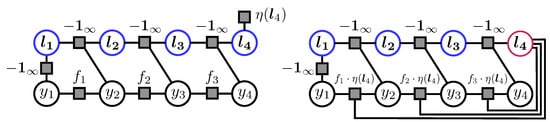
Figure 2.
Factor graph representation for an augmented objective for margin scaling (on the left) and for slack scaling (on the right). The auxiliary variables are marked in blue (except for slack scaling). is the hub node.
Applying the same scheme for slack scaling yields a much more sparsely connected graph (see the rightmost graph in Figure 2). This is achieved by forcing the majority of connections to go through a single node , which we call a hub node. Actually, becomes 2-decomposable if we fix the value of , which then can be multiplied into the corresponding factors of F. In this way, we can effectively reduce the overall treewidth at the expense of increased polynomial computation time (compared to a chain without the global factor), provided that the maximal number R of different states of each auxiliary variable is polynomially bounded in M, which represents the number of nodes in the original graph. In the context of training SSVMs, for example, the majority of the popular loss functions satisfy this condition (see Table 1 in Section 5 for an overview).
3.2. Constrained Message-Passing Algorithm on Clique Trees
The idea presented in the previous section is intuitive and enables the reuse of existing software. Specifically, we can use the conventional junction-tree algorithm for graphical models by extending the original graph with nodes corresponding to the auxiliary variables. Alternatively, instead of performing an explicit graph transformation, we can modify the message-passing protocol, which is asymptotically at least one order of magnitude faster. Therefore, we do not explicitly introduce auxiliary variables as graph nodes before constructing the clique tree but rather use them to condition the message-passing rules. In the following, we derive an algorithm for solving an instance of Problem 1 via constrained message passing on clique trees. The resulting computational scheme can be seen as a direct extension of the junction-tree algorithm to models with specific global factors. Note that the form of tractable global dependencies is constrained according to the definition of Problem 1.
First, similar to the conventional junction-tree algorithm, we need to construct a clique tree for a given set of factors that preserves the family structure and has the running intersection property. Note that we ignore the global term during this process. The corresponding energy is given by the function F according to the definition of Problem 1. There are two equivalent approaches for constructing the click tree [1,70]. The first is based on variable elimination and the second is based on graph triangulation, with an upper bound of . Figure 3 illustrates the intermediate steps of the corresponding construction process for a given factor graph using the triangulation approach. The resulting clique tree example defines the starting point for our message-passing algorithm.
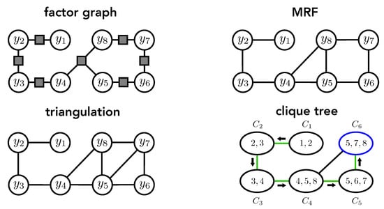
Figure 3.
Illustration of the transformation process of a factor graph into a clique tree. The upper-left graph represents the original factor graph, which describes how the energy of the model without the global factor (see F in the definition of Problem 1) factorizes over the individual variables. In the first step, the factor graph is transformed into an MRF, as shown in the upper-right graph. The lower-left graph shows the result of triangulating the MRF from the previous step. Finally, the lower-right graph shows the resulting cluster graph with cliques constructed from the triangulated MRF. The numbers within the cluster nodes denote the variable indices belonging to the corresponding clique (e.g., refers to ). The green edges indicate a valid spanning clique tree extracted from the cluster graph. The dark arrows represent one possible order of message passing if clique (marked blue) has been chosen as the root of the clique tree.
Assume that a clique tree with cliques is given, where denotes a set of indices of variables contained in the i-th clique. We denote a corresponding set of variables by . Furthermore, we use the notations and to denote the clique potentials (or factors) related to the mappings F and in the definition of Problem 1, respectively. Additionally, we denote by a clique chosen to be the root of the clique tree. Finally, we use the notation for the indices of the neighbors of the clique . We can now compute the optimal value of the objective in Problem 1 as follows. Starting at the leaves of the clique tree, we iteratively send messages toward the root according to the following message-passing protocol. A clique can send a message to its parent clique if it received all messages from the rest of its neighbors for . In that case, we say that is ready.
For each configuration of the variables and parameters (encoding the state of an auxiliary variable associated with the current clique ), a corresponding message from a clique to a clique can be computed according to the following equation:
where we maximize over all configurations of the variables and over all parameters subject to the following constraint
This means that each clique is assigned exactly one (multivariate) auxiliary variable and the range of possible values can take on is implicitly defined by Equation (8). After resolving the recursion in the above equation, we can see that the variable corresponds to a sum of the potentials for each previously processed clique in a subtree of the graph of which forms the root. We refer to Equation (4) in the previous subsection for comparison.
| Algorithm 1 Constrained Message Passing on a Clique Tree |
|
The algorithm terminates if the designated root clique received all messages from its neighbors. We then compute the values
maximizing over all configurations of , and subject to the constraint , which we use to obtain the optimal value of Problem 1 according to
The corresponding optimal solution of Problem 1 can be obtained by backtracking the additional variables , saving optimal decisions in intermediate steps. The complete algorithm is summarized in Algorithm 1. As an alternative, we provide an additional flowchart diagram illustrating the algorithmic steps in Appendix B (see Figure A1 for further details). We underline this important result by the following theorem, for which we provide the proof in Appendix A. It should be noted that this theorem refers to the more general target objective defined in Problem 1 and should replace the corresponding statement in Theorem 2 in [69].
Theorem 1.
Algorithm 1 always finds an optimal solution to Problem 1. The computational complexity is of the order , where R denotes an upper bound on the number of states of each auxiliary variable, and ν is defined as the maximal number of neighbors of a node in a corresponding clique tree.
Besides the treewidth , the value of the parameter also appears to be crucial for the resulting running time of Algorithm 1 since the corresponding complexity is also exponential in . The following proposition suggests that among all possible cluster graphs for a given MRF, there always exists a clique tree for which tends to take on small values (provided is small) and effectively does not depend on the size of the corresponding MRF. We provide the proof in Appendix C.
Proposition 2.
For any MRF with treewidth τ, there is a clique tree for which the maximal number of neighbors of each node is upper bounded according to .
To support the above proposition, we consider the following extreme example, which is illustrated in Figure 4. We are given an MRF with a star-like shape (on the left) with variables and treewidth . One valid clique tree for this MRF is shown in the middle. In particular, the clique containing the variables has neighbors. Therefore, running Algorithm 1 on that clique tree results in a computational time exponential in the graph size M. However, it is easy to modify that clique tree to have a small number of neighbors for each node (shown on the right), upper bounded by .
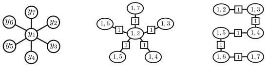
Figure 4.
Illustration of an extreme example where can be linear in the graph size. The leftmost graph represents an MRF with variables and treewidth . The graph in the middle shows a valid clique tree for the MRF on the left, where the clique has neighbors, that is, is linear in the graph size for that clique tree. The rightmost graph represents another clique tree that has a chain form, where . The squared nodes denote the corresponding sepsets.
Although Proposition 2 assures the existence of a clique tree with a small , the actual upper bound on is still very pessimistic (exponential in the treewidth). In fact, by allowing a simple graph modification, we can always reduce the -parameter to a small constant (). Specifically, we can clone each cluster node with more than three neighbors multiple times so that each clone only carries one of the original neighbors. We then connect the clones by a chain that preserves the running intersection property. To ensure that the new cluster graph describes the same set of potentials we set the potentials for each copy of a cluster node to zero: and . The complete modification procedure is illustrated in Figure 5. We summarize this result in the following corollary.
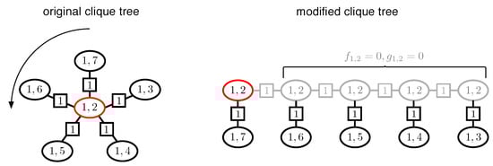
Figure 5.
Illustration of a modification procedure to reduce the maximal number of neighbors for each cluster node in a given clique tree. The graph on the left represents an original clique tree. The only node with more than three neighbors is marked in red. We clone this cluster node multiple times so that each clone only carries one of the original neighbors. The clones are connected by a chain that preserves the running intersection property. The arrow in the left graph indicates the (arbitrarily chosen) order of processing the neighbor nodes. The graph resulting from this transformation is shown on the right. The clones in the new graph are marked in gray. To ensure that the new cluster graph describes the same set of potentials, we set the potentials for the copies of each cloned cluster node to zero: and . This procedure reduces the -parameter to a constant (), significantly reducing the computational cost.
Corollary 1.
Provided a given clique tree is modified according to the presented procedure for reducing the number of neighbors for each cluster node, the overall computational complexity of running Algorithm 1 (including time for graph modification) is of the order .
Note that in the case where the corresponding clique tree is a chain, the resulting complexity reduces to . At this point, we would like to provide an alternative perspective of the computational complexity in this case (with , ), which shows the connection to the conventional junction-tree algorithm. Specifically, the constrained message-passing algorithm (Algorithm 1) can be seen as conventional message passing on a clique tree (for the mapping F in Problem 1) without auxiliary variables, but with an increased size of the state space for each variable , from N to . Then, Proposition 1 guarantees an exact inference in time of the order . The summation constraints with respect to the auxiliary variables can be ensured by extending the corresponding potential functions to take on , forbidding inconsistent state transitions between individual variables. The same observation holds for message passing on factor graphs. To summarize, by introducing auxiliary variables, we can remove the global dependencies imposed by the mapping H in Problem 1, thereby reducing the overall treewidth. However, this comes at the cost of the label space becoming a function of the graph size (R is usually dependent on M).
We conclude our discussion by analyzing the relation between the maximal number of states (of the auxiliary variables) R and the number of variables M in the original MRF. In the worst case, R can grow exponentially with the graph size M. This happens, for example, when the values that the individual factors can take on are scattered across a very large range that grows much faster relative to the graph size. For practical cases, however, we can assume that the individual factor functions take values in an integer interval, which is either fixed or grows polynomially with the graph size. In that case, R is always a polynomial in M, rendering the overall complexity of Algorithm 1 a polynomial in the graph size, as we demonstrate with several examples in Section 6. We summarize this in the following theorem. The corresponding proof is given in Appendix D.
Theorem 2.
Consider an instance of Problem 1 given by a clique tree with M variables. Let be a number that grows polynomially with M. Provided each factor in a decomposition of assumes values from a discrete set of integers , the number R grows polynomially with M according to .
4. Application Use Cases
In this section, we demonstrate the expressivity of Problem 1 by showcasing the diversity of existing (and potentially new) applications that align with our target objective. In particular, practitioners can gain insight into specific examples to verify whether a given task is an instance of Problem 1. The research conducted within the scope of this paper has been motivated by the following use cases:
- Learning with High-Order Loss FunctionsSSVM enables building complex and accurate models for structured prediction by directly integrating the desired performance measure into the training objective. However, its applicability relies on the availability of efficient inference algorithms. In the state-of-the-art training algorithms, such as cutting planes [64,65], bundle methods [67,68], subgradient methods [18], and Frank–Wolfe optimization [66], inference is repeatedly performed either to compute a subgradient or find the most violating configuration. In the literature, the corresponding computational task is generally referred to as the loss-augmented inference, which is the main computational bottleneck during training.
- Enabling Training of Slack Scaling Formulation for SSVMsThe maximum-margin framework of SSVMs includes two loss-sensitive formulations known as margin scaling and slack scaling. Since the original paper on SSVMs [39], there has been much speculation about the differences in training using either of these two formulations. In particular, training via slack scaling has been conjectured to be more accurate and beneficial than margin scaling. Nevertheless, it has rarely been used in practice due to the lack of known efficient inference algorithms.
- Evaluating Generalization Bounds for Structured PredictionThe purpose of generalization bounds is to provide useful theoretical insights into the behavior and stability of a learning algorithm by upper bounding the expected loss or the risk of a prediction function. Evaluating such a bound could provide certain guarantees on how a system trained on some finite data will perform in the future on unseen examples. Unlike in standard regression or classification tasks with univariate real-valued outputs, in structured prediction, evaluating generalization bounds requires solving a combinatorial optimization problem, thereby limiting its use in practice [48].
- Globally Constrained MAP InferenceIn many cases, evaluating a prediction function with structured outputs technically corresponds to performing MAP inference on a discrete graphical model, including Markov random fields (MRFs) [1], probabilistic context-free grammars (PCFGs) [72,73,74], hidden Markov models (HMMs) [75], conditional random fields (CRFs) [3], probabilistic relational models (PRMs) [76,77], and Markov logic networks (MLNs) [78]. In practice, we might want to modify the prediction function by imposing additional (global) constraints on its output. For example, we could perform a corresponding MAP inference subject to the constraints on the label counts specifying the size of the output or the distribution of the resulting labels, which is a common approach in applications such as sequence tagging and image segmentation. Alternatively, we might want to generate the best output with a score from a specific range that can provide deeper insights into the energy function of a corresponding model. Finally, we might want to restrict the set of possible outputs directly by excluding specific label configurations. The latter is closely related to the computational task known as (diverse) k-best MAP inference [62,63].
In the following, we provide technical details about how the generic tasks listed above can be addressed using our framework.
4.1. Loss-Augmented Inference with High-Order Loss Functions
As already mentioned, Problem 1 covers as a special case the task of loss-augmented inference (for margin and slack scaling) within the framework of SSVM [39,46]. In order to match the generic representation given in (2), we can define , and for suitable and . Here, denotes a joint feature map on an input–output pair , is a trainable weight vector, and is a dissimilarity measure between a prediction and a true output . Given this notation, our target objective can be written as follows:
We note that a considerable number of non-decomposable (or high-order) loss functions in structured prediction can be represented as multivariate cardinality-based potentials , where the mapping encodes the label statistics, e.g., the number of true or false positives with respect to the ground truth. Furthermore, the maximal number of states R for the corresponding auxiliary variables related to is polynomially bounded in the number of variables M (see Table 1 in Section 5 for an overview of existing loss functions and the resulting values for R). For the specific case of a chain graph with -loss, for example, the resulting complexity of Algorithm 1 is cubic in the graph size.
4.2. Evaluating Generalization Bounds in Structured Prediction
In the following, we demonstrate how our algorithmic idea can be used to evaluate the PAC-Bayesian generalization bounds for max-margin structured prediction. As a working example, we consider the following generalization theorem, as stated in [48]:
Theorem 3.
Assume that . With a probability of at least over the draw of the training set of size , the following holds simultaneously for all weight vectors :
where denotes the corresponding prediction function.
Evaluating the second term on the right-hand side of the inequality in (12) involves a maximization over for each data point according to
We now show that this maximization term is an instance of Problem 1. More precisely, we consider an example with and an -loss (see Table 1). Next, we define , , and set
where we use , , which removes the need for additional auxiliary variables for the Hamming distance, reducing the resulting computational cost. Here, , , and denote the numbers of true positives, false positives, and false negatives, respectively. denotes the size of the output . Both and are constant with respect to the maximization over . Note also that H is non-decreasing in . Furthermore, the number of states of the auxiliary variables is upper bounded by (see Table 1). Therefore, here, the computational complexity of Algorithm 1 (according to Corollary 1) is given by .
As a final remark, we note that training an SSVM corresponds to solving a convex problem but is not consistent. It fails to converge to the optimal predictor even in the limit of infinite training data (see [60] for more details). However, minimizing the (non-convex) generalization bound is consistent. Algorithm 1 provides an effective evaluation tool that could potentially be used for the development of new training algorithms based on the direct minimization of such bounds. We leave the corresponding investigation for future work.
4.3. Globally-Constrained MAP Inference
Another common use case is performing MAP inference on graphical models (such as MRFs) subject to additional constraints on the variables or the range of the corresponding objective including various tasks such as image segmentation in computer vision, sequence tagging in computational biology or natural language processing, and signal denoising in information theory. We note that an important tractability assumption in the definition of Problem 1 is the -decomposability of F and with a reasonably small treewidth . In areas such as computer vision, we usually encounter models (e.g., Ising grid model) where the treewidth is a function of the graph size given by . In this case, we can use Algorithm 1 by leveraging the technique of dual decomposition [5,16,79]. More precisely, we decompose the original graph in (multiple) trees, where the global factor is attached to exactly one of the trees in our decomposition. We also note that from a technical perspective, the problem of MAP inference subject to some global constraints on the statistics is equivalent to the MAP problem augmented with a global cardinality-based potential . Specifically, we can define as an indicator function , which returns if the corresponding constraint on is violated. Furthermore, the form of does not affect the message passing of the presented algorithm. We can always check the validity of a corresponding constraint after all the necessary statistics have been computed.
4.3.1. Constraints on Label Counts
As a simple example, consider the binary-sequence tagging experiment, that is, every output is a sequence, and each site in the sequence can be either 0 or 1. Given some prior information on the number b of positive labels, we can improve the quality of the results by imposing a corresponding constraint on the outputs:
We can write this as an instance of Problem 1 by setting
where , and . Since all the variables in are binary, the number of states R of the corresponding auxiliary variables is upper bounded by M. In addition, because the output graph is a sequence, we have , . Therefore, here, the computational complexity of Algorithm 1 is of the order .
4.3.2. Constraints on Objective Value
We continue with the binary-sequence tagging example (with pairwise interactions). To force constraints on the score to be in a specific range, as in
we first rewrite the prediction function in terms of its sufficient statistics according to
, , and define
Note that contains all the sufficient statistics of F such that . Here, we could replace with any (non-linear) constraint on the sufficient statistics of the joint feature map .
The corresponding computational complexity can be derived by considering an urn problem: one with and one with distinguishable urns and M indistinguishable balls. Here, D denotes the size of the dictionary for the observations in the input sequence . Note that the dictionary of the input symbols can be large compared to other problem parameters. However, we can reduce D to the size of the vocabulary only occurring in the current input . The first urn problem corresponds to the unary observation-state statistics , and the second corresponds to the pairwise statistics for the state transition . The resulting number of possible distributions of balls over the urns is given by
Although the resulting complexity (due to ) being is still a polynomial in the number of variables M, the degree is quite high, making it suitable for only short sequences. For practical use, we recommend the efficient approximation framework of Lagrangian relaxation and Dual Decomposition [5,16,79].
4.3.3. Constraints on Search Space
The constraints on the search space can be different from the constraints we can impose on the label counts. For example, we might want to exclude a set of K complete outputs from the feasible set by using an exclusion potential .
For simplicity, we again consider a sequence-tagging example with pairwise dependencies. Given a set of K patterns to exclude, we can introduce auxiliary variables , where for each pattern , we have a constraint . More precisely, we modify the message computation in (7) with respect to the auxiliary variables by replacing the corresponding constraints in the maximization over with the constraints . Therefore, the maximal number of states for is given by . The resulting complexity for finding an optimal solution over is of the order .
A related problem is finding a diverse k-best solution. Here, the goal is to produce the best solutions that are sufficiently different from each other according to a diversity function, e.g., a loss function such as the Hamming distance . More precisely, after computing the MAP solution , we compute the second-best (diverse) output with . For the third-best solution, we then require and , and so on. In other words, we search for an optimal output such that , for all .
For this purpose, we define auxiliary variables , where for each pattern , we have a constraint , which computes the Hamming distance of a solution with respect to the pattern . Therefore, we can define
where , and at the final stage (due to ), we have all the necessary information to evaluate the constraints with respect to the diversity function (here Hamming distance). The maximal number of states R for the auxiliary variables is upper bounded by . Therefore, the resulting running time for finding the K-th diverse output sequence is of the order .
Finally, we note that the concept of diverse K-best solutions can also be used during the training of SSVMs to speed up the convergence of a corresponding algorithm by generating diverse cutting planes or subgradients, as described in [63]. An appealing property of Algorithm 1 is that we obtain some of the necessary information for free as a side effect of the message passing.
5. Compact Representation of Loss Functions
We now further advance the task of loss-augmented inference (see Section 4.1) by presenting a list of popular dissimilarity measures that our algorithm can handle, which are summarized in Table 1. The measures are given in a compact representation based on the corresponding sufficient statistics encoded as a mapping . Columns 2 and 3 show the form of and , respectively. Column 4 provides an upper bound R on the number of possible values of auxiliary variables that affect the resulting running time of Algorithm 1 (see Corollary 1).

Table 1.
Compact representation of popular dissimilarity measures based on the corresponding sufficient statistics . The upper (and lower!) bounds on the number of states of the auxiliary variables R for the presented loss functions are shown in the last column.
Table 1.
Compact representation of popular dissimilarity measures based on the corresponding sufficient statistics . The upper (and lower!) bounds on the number of states of the auxiliary variables R for the presented loss functions are shown in the last column.
| Loss | R | ||
|---|---|---|---|
| G | M | ||
| M | |||
| G | M | ||
| M | |||
| M | |||
| G | M | ||
Here, denotes the number of nodes in the output . , and are the numbers of true positives, false positives, and false negatives, respectively. The number of true positives for a prediction and a true output is defined as the number of common nodes with the same label. The number of false positives is determined by the number of nodes that are present in the output but missing (or with another label) in the true output . Similarly, the number of false negatives corresponds to the number of nodes present in but missing (or with another label) in . In particular, it holds that .
We can see in Table 1 that each element of is a sum of binary variables, which significantly reduces the image size of mapping . This occurs despite the exponential variety of the output space . As a result, the image size grows only polynomially with the size of the outputs , and the number R provides an upper bound on the image size of .
Zero-One Loss ()
This loss function takes on binary values and is the most uninformative since it requires a prediction to match the ground truth to 100% and provides no partial quantification of the prediction quality in the opposite case. Technically, this measure is not decomposable since it requires the numbers of and to be evaluated via
Sometimes, we cannot compute the (unlike ) from the individual nodes of a prediction. Instead, we can count the and compute the using the relationship . For example, if the outputs are set with no ordering indication of the individual set elements, we need to know the whole set in order to be able to compute the . Therefore, computing from a partially constructed output is not possible. We note, however, that in the case of the zero-one loss function, there is a faster inference approach, which involves modifying the prediction algorithm to also compute the second-best output and selecting the best result based on the value of the objective function.
Hamming Distance/Hamming Loss ()
In the context of sequence learning, given a true output and a prediction of the same length, the Hamming distance measures the number of states on which the two sequences disagree:
By normalizing this value, we obtain the Hamming loss, which does not depend on the length of the sequences. Both measures are decomposable.
Weighted Hamming Distance ()
For a given matrix , the weighted Hamming distance is defined as . However, keeping track of the accumulated sum of the weights until the current position t in a sequence, unlike for the Hamming distance, can be intractable. We can, however, use the following observation. It is sufficient to count the occurrences for each pair of states according to
In other words, each dimension of (denoted as ) corresponds to
Here, we can upper bound the image size of by considering an urn problem with distinguishable urns and M indistinguishable balls. The number of possible distributions of the balls over the urns is given by .
False Positives/Precision/Recall ()
False positives measure the discrepancy between outputs by counting the number of false positives in a prediction with respect to the true output . This metric is often used in learning tasks such as natural language parsing due to its simplicity. Precision and recall are popular measures used in information retrieval. By subtracting the corresponding values from one, we can easily convert them to a loss function. Unlike precision given by , recall effectively depends on only one parameter. Although it is originally parameterized by two parameters given as , we can exploit the fact that the value is always known in advance during the inference, rendering recall a decomposable measure.
-Loss ()
The -score is often used to evaluate performance in various natural language processing applications and is also suitable for many structured prediction tasks. It is originally defined as the harmonic mean of precision and recall
However, since the value is always known in advance during the inference, the -score effectively depends on only two parameters . The corresponding loss function is defined as .
Intersection Over Union ()
The Intersection-Over-Union loss is mostly used in image processing tasks such as image segmentation and object recognition and was used as a performance measure in the Pascal Visual Object Classes Challenge [80]. It is defined as . We can easily interpret this value in cases where the outputs , describe the bounding boxes of pixels. The more the overlap of two boxes, the smaller the loss value. We note that in the case of binary image segmentation, for example, we have a different interpretation of true and false positives. In particular, it holds that , where is the number of positive entries in . In terms of the contingency table, this yields
Since , the value effectively depends on only two parameters (instead of three). Moreover, unlike -loss, defines a proper distance metric on sets.
Label-Count Loss ()
The Label-Count loss is a performance measure used for the task of binary image segmentation in computer vision and is given by
This loss function prevents assigning low energy to segmentation labelings with substantially different areas compared to the ground truth.
Number/Rate of Crossing Brackets (, )
The number of Crossing Brackets () is a measure used to evaluate performance in natural language parsing. It computes the average of how many constituents in one tree cross over constituent boundaries in the other tree . The normalized version (by ) of this measure is called the Crossing Brackets (Recall) Rate. Since the value is not known in advance, the evaluation requires a further parameter for the size of .
Bilingual Evaluation Understudy ()
Bilingual Evaluation Understudy, or BLEU for short [81], is a measure used to evaluate the quality of machine translations. It computes the geometric mean of the precision of k-grams of various lengths (for ) between a hypothesis and a set of reference translations, multiplied by a factor to penalize short sentences according to
Note that K is a constant, rendering the term a polynomial in M.
Recall-Oriented Understudy for Gisting Evaluation (, )
The Recall-Oriented Understudy for Gisting Evaluation, or ROUGE for short [82], is a measure used to evaluate the quality of a summary by comparing it to other summaries created by humans. More precisely, for a given set of reference summaries and a summary candidate X, ROUGE-K computes the percentage of k-grams from that appear in X according to
where provides the number of occurrences of a k-gram k in a summary S. We can estimate an upper bound R on the image size of similarly to the derivation for the weighted Hamming distance above as , where is the dimensionality of . This represents the number of unique k-grams occurring in the reference summaries. Note that we do not need to count grams that do not occur in the references.
Another version, ROUGE-LCS, is based on the concept of the longest common subsequence (LCS). More precisely, for two summaries X and Y, we first compute , which is the length of the LCS. We then use this value to define precision and recall measures given by and , respectively. These measures are used to evaluate the corresponding F-measure:
In other words, each dimension in is indexed by an . ROUGE-LCS (unlike ROUGE-K) is non-decomposable.
6. Validation of Theoretical Time Complexity
To demonstrate feasibility, we evaluate the performance of our algorithm on several application tasks: part-of-speech tagging [83], base-NP chunking [84], and constituency parsing [39,46]. More precisely, we consider the task of loss-augmented inference (see Section 4.1) for margin and slack scaling with different loss functions. The run-times for the task of diverse k-best MAP inference (Section 4.3) and for evaluating the structured generalization bounds (see Section 4.2) are identical to the run-time for the loss-augmented inference with slack scaling. We omit the corresponding plots due to redundancy. In all the experiments, we used Penn English Treebank-3 [85] as a benchmark data set, which provides a large corpus of annotated sentences from the Wall Street Journal. For better visualization, we restrict our experiments to sentences containing at most 40 words. The resulting time performance is shown in Figure 6. We can see that different loss functions result in different computation costs, as indicated by the number of values for the auxiliary variables shown in the last column of Table 1. In particular, the shapes of the curves are consistent with the upper bound provided in Theorem 1, which reflects the polynomial degree of the overall dependency with respect to the graph size M. The difference between margin and slack scaling is due to the fact that in the case of a decomposable loss function , the corresponding loss terms can be folded into the factors of the compatibility function F, allowing for the use of conventional message passing.
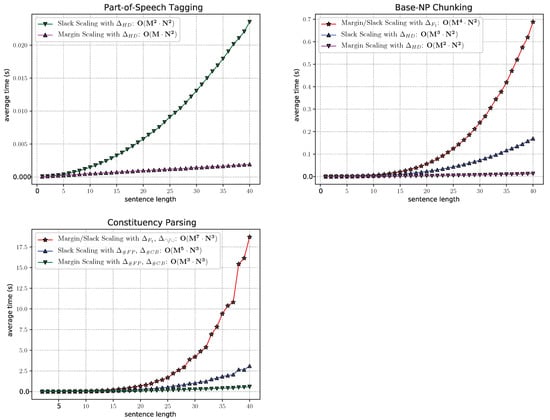
Figure 6.
Empirical evaluation of the run-time performance of loss-augmented inference for part-of-speech tagging, base-NP chunking, and constituency-parsing tasks.
7. Summary of Contributions
In this paper, we provided a set of formal contributions by generalizing the idea of constrained message passing introduced in [69]. Our improved framework, which is presented in this paper, includes the following key elements:
- Abstract definition of the target problem (see Problem 1);
- Constrained message-passing algorithm on clique trees (see Algorithm 1);
- Formal statements to ensure theoretical properties such as correctness and efficiency (see Theorem 1, Proposition 2, Corollary 1, Theorem 2).
We emphasize that the idea of using auxiliary variables to constrain message passing is not novel per se and was originally proposed in [69]. Our first contribution concerns the difference in the definition of the target problem, which broadens the range of admissible applications. More precisely, the target objective H in the previous publication relates the energy of the model F and the vector-valued mapping , which describes the sufficient statistics of the global terms in a rather restricted form according to
where is a non-negative function on . Although this is sufficient for the purposes of [69], there are other computational problems that could benefit from the same message-passing idea but cannot be addressed by it in the above form. Therefore, we relax the form of the function H in our target problem (Problem 1) to allow much finer interactions between F and . Specifically, we allow H to be any function on the arguments , which is restricted only by the requirement that it is non-decreasing in the first argument. Without this assumption, the proposed algorithm (Algorithm 1) is not guaranteed to provide an optimal solution. Therefore, all related theorems, algorithms, and the corresponding proofs in [69] must be adjusted accordingly. Conceptually, we can reuse the computational core idea, including the introduction of auxiliary variables, without any changes. The only difference in the new version of the algorithm is how the statistics gathered during message passing are evaluated at the end to ensure the optimality of the solution according to the new requirement on the function H (see line 8 in Algorithm 1). In order to motivate the significance and practical usability of this extension, we demonstrated that mappings F and can interact by means of the function H in a highly non-trivial way, thereby exceeding the range of problem formulations in [69]. In particular, we showed how the generalization bounds in structured prediction can be evaluated using our approach (see Section 4.2). To the best of our knowledge, there are no existing methods for finding an optimal solution for this task.
Our second contribution involves a new graph transformation technique via node cloning (illustrated in Figure 5), which significantly enhances the asymptotic bounds on the computational complexity of Algorithm 1. Previously, in [69], the polynomial running time was guaranteed only if the maximal node degree in a corresponding cluster graph was bounded by a (small) constant. The proposed transformation effectively removes this limitation and ensures polynomial running time regardless of the graph structure. We emphasize this result in Corollary 1. Note that the term in Theorem 1 in [69] has been replaced with in Corollary 1 of the current paper, thereby reducing the computational complexity of the resulting message-passing algorithm. This reduction is significant, as can be dependent on the graph size in the worst case (see Figure 4).
As our third contribution, we investigate the important question of how the parameter R, which describes the maximum number of states for auxiliary variables, grows with the size of the graph, as measured by the total number of variables M in the corresponding MRF. As a result, we identify a sufficient condition on that guarantees the overall polynomial run-time of Algorithm 1 in relation to the graph size in our target problem (Problem 1; see Theorem 2).
8. Related Works
Several previous works have addressed the problem of exact MAP inference with global factors in the context of SSVMs when optimizing for non-decomposable loss functions. Joachims [86] proposed an algorithm for a set of multivariate losses, including the -loss. However, the presented idea applies only to a simple case, where the corresponding mapping F in (2) decomposes into non-overlapping components (e.g., unary potentials).
Similar ideas based on the introduction of auxiliary variables have been proposed [87,88] to modify the belief propagation algorithm according to a special form of high-order potentials. Specifically, for the case of binary-valued variables , the authors focus on the univariate cardinality potentials. For the tasks of sequence tagging and constituency parsing, ref. [45,46] propose an exact inference algorithm for the slack scaling formulation that focuses on the univariate dissimilarity measures and (see Table 1 for details). In [69] the authors extrapolate this idea and provide a unified strategy to tackle multivariate and non-decomposable loss functions.
In the current paper, we build on the results in [69] and generalize the target problem (Problem 1) by increasing the range of admissible applications. More precisely, we replace the binary operation corresponding to either a summation or multiplication in the previous objective with a function , thereby allowing for more subtle interactions between the energy of the core model F and the sufficient statistics according to . The increased flexibility, however, must be further restricted in order for a corresponding solution to be optimal. We have found that it is sufficient to impose a requirement on H to be non-decreasing in the first argument. Note that for the special case of the objective in [69], this requirement automatically holds.
Furthermore, the previous works could only guarantee polynomial run-time in cases where (a) the core model can be represented by a tree-shaped factor graph, and (b) the maximal degree of a variable node in the factor graph is bounded by a constant. The former excludes problems with cyclic dependencies and the latter rejects graphs with star-like shapes. The corresponding idea for clique trees can handle cycles but suffers from a similar restriction on the maximal node degree being bounded. Here, we solve this problem by applying the graph transformation proposed in Section 3.2, effectively reducing the maximal node degree to . We note that a similar idea can be applied to factor graphs by replicating variable nodes and introducing constant factors. As a result, we improve the guarantee on the computational complexity by reducing the potentially unbounded parameter in the upper bound to .
In future work, we will consider applying our framework to the explanation task based on the technique of layer-wise relevance propagation [89] in graph neural networks, following in the spirit of [90,91].
9. Conclusions
Despite the high diversity in the range of existing applications, a considerable number of the underlying MAP problems share the unifying property that the information on the global variable interactions imposed by either a global factor or a global constraint can be locally propagated through the network by means of dynamic programming. By extending previous works, we presented a theoretical framework for efficient exact inference on models involving global factors with decomposable internal structures. At the heart of the presented framework is a constrained message-passing algorithm that always finds an optimal solution for our target problem in polynomial time. In particular, the performance of our approach does not explicitly depend on the graph form but rather on intrinsic properties such as the treewidth and the number of states of the auxiliary variables defined by the sufficient statistics of global interactions. The overall computational procedure is provably exact, and it has lower asymptotic bounds on the computational time complexity compared to previous works.
Author Contributions
Conceptualization, A.B.; Methodology, A.B.; Software, A.B.; Validation, A.B.; Formal analysis, A.B. and S.N.; Investigation, A.B.; Writing—original draft, A.B.; Writing—review & editing, A.B., S.N. and K.-R.M.; Funding acquisition, K.-R.M. All authors have read and agreed to the published version of the manuscript.
Funding
A.B. acknowledges support by the BASLEARN—TU Berlin/BASF Joint Lab for Machine Learning, cofinanced by TU Berlin and BASF SE. S.N. and K.-R.M. acknowledge support by the German Federal Ministry of Education and Research (BMBF) for BIFOLD under grants 01IS18025A and 01IS18037A. K.-R.M. was partly supported by the Institute of Information and Communications Technology Planning and Evaluation (IITP) grants funded by the Korea government(MSIT) (no. 2019-0-00079, Artificial Intelligence Graduate School Program, Korea University and no. 2022-0-00984, Development of Artificial Intelligence Technology for Personalized Plug-and-Play Explanation and Verification of Explanation) and by the German Federal Ministry for Education and Research (BMBF) under grants 01IS14013B-E and 01GQ1115.
Data Availability Statement
The data used in the experimental part of this paper is available at https://catalog.ldc.upenn.edu.
Conflicts of Interest
The authors declare no conflict of interest. The funders had no role in the design of the study; in the collection, analyses, or interpretation of data; in the writing of the manuscript; or in the decision to publish the results.
Abbreviations
The following abbreviations are used in this manuscript:
| LCS | Longest Common Subsequence |
| MAP | Maximum A Posteriori |
| MRF | Markov Random Field |
| SSVM | Structural Support Vector Machine |
Appendix A. Proof of Theorem 1
Proof.
We now show the correctness of the presented computations. For this purpose, we first provide a semantic interpretation of messages as follows. Let be an edge in a clique tree. We denote by the set of clique factors of the mapping F on the -th side of the tree, and by the corresponding set of clique factors of the mapping . Furthermore, we denote by the set of all variables appearing on the -th side but not in the sepset . Intuitively, a message sent from clique to corresponds to the sum of all factors contained in , which is maximized (for fixed values of and ) over the variables in subject to the constraint . In other words, we define the following induction hypothesis:
Now, consider an edge such that is not a leaf. Let be the neighboring cliques of other than . It follows from the running intersection property that is a disjoint union of for and the variables eliminated at itself. Similarly, is the disjoint union of the and . Finally, is the disjoint union of the and . In the following, we abbreviate the term describing a range of variables in subject to the corresponding equality constraint with respect to by . Thus, the right-hand side of Equation (A1) is equal to
where in the second max, we maximize over all configurations of subject to the constraint . Since all the corresponding sets are disjoint, the term (A2) is equal to
where, again, the maximization over is subject to the constraint . Using the induction hypothesis in the last expression, we obtain the right-hand side of Equation (7), thereby proving the claim in Equation (A1).
Now, look at Equation (9). By using Equation (A1) and considering that all the sets of variables and factors involved in different messages are disjoint, we can conclude that the computed values correspond to the sum of all factors f for the mapping F over the variables in , which is maximized subject to the constraint . Note that up until now, the proof is equivalent to that provided for Theorem 2 in the previous publication [69] because the message-passing step constrained via auxiliary variables is identical. Now, we use an additional requirement on H to ensure the optimality of the corresponding solution. Because H is non-decreasing in the first argument, by performing maximization over all values according to Equation (10), we obtain the optimal value of Problem 1.
By inspecting the formula for the message passing in Equation (7), we can conclude that the corresponding operations can be performed in time, where denotes the maximal number of neighbors of any clique node . First, the summation in Equation (7) involves terms, resulting in summation operations. Second, a maximization is performed first over variables with a cost . This, however, is carried out for each configuration of , where , resulting in . Then, a maximization over costs an additional . Together with the possible values for , it yields , where we upper bound by . Therefore, sending a message for all possible configurations of on the edge costs time. Finally, we need to carry out these operations for each edge in the clique tree. The resulting cost can be estimated as follows: , where V denotes the set of clique nodes in the clique tree. Therefore, the total complexity is upper bounded by . □
Appendix B. Flowchart Diagram of Algorithm 1
We present a flowchart diagram for Algorithm 1 in Figure A1.

Figure A1.
Flowchart diagram for Algorithm 1 for implementing a constrained message-passing scheme on clique trees. Algorithm 1 is guaranteed to always find an optimal solution in polynomial time. Its computational complexity is upper bounded according to .
Appendix C. Proof of Proposition 2
Proof.
Assume we are given a clique tree with treewidth . This means that every node in the clique tree has at most variables. Therefore, the number of all possible sepsets for a clique, which refers to the number of all variable combinations shared between two neighbors, is given by , where we exclude the empty set and the set containing all the variables in the corresponding clique.
Furthermore, we can deal with sepset duplicates by iteratively rearranging the edges in the clique tree such that for every sepset from the possibilities, there is at most one duplicate providing an upper bound of on the number of edges for each node. More precisely, we first choose a node with more than neighbors as the root and then reshape the clique tree by propagating some of the duplicate edges (together with the corresponding subtrees) toward the leaves, as illustrated in Figure A2. The duplicate edges of nodes connected to the leaves of the clique tree can be reattached in a sequential manner similar to the example shown in Figure 4. Due to this procedure, the maximal number of duplicates for every sepset is upper bounded by 2. Multiplied by the maximal number of possible sepsets for each node, we obtain an upper bound on the number of neighbors in the reshaped clique tree given by . □

Figure A2.
Illustration of the reshaping procedure for a clique tree in the case where the condition is violated. is the root clique where a sepset a occurs at least two times. The number of neighbors of can be reduced by removing the edge between and and attaching to . In this way, we can ensure that every node has at most one duplicate for every possible sepset. Furthermore, this procedure preserves the running intersection property.
Appendix D. Proof of Theorem 2
Proof.
We provide the proof by induction. Let be the cliques of a corresponding instance of Problem 1. We now consider an arbitrary but fixed order of for . We denote by the number of states of a variable , that is, R is given by . As previously mentioned (see Equation (8)), an auxiliary variable corresponds to the sum of potentials over all in a subtree of which is the root. This means that the number is upper bounded by the image size of the corresponding sum function according to
where the corresponding values are in the set , defining our induction hypothesis. Using the induction hypothesis and the assumption , it directly follows that the values for are all in the set . The base case for holds due to the assumption of the theorem. Because always holds and the order of the considered cliques is arbitrary, we can conclude that R is upper bounded by , which is a polynomial in M. □
References
- Koller, D.; Friedman, N. Probabilistic Graphical Models: Principles and Techniques-Adaptive Computation and Machine Learning; The MIT Press: Cambridge, MA, USA, 2009. [Google Scholar]
- Wainwright, M.J.; Jordan, M.I. Graphical Models, Exponential Families, and Variational Inference. Found. Trends Mach. Learn. 2008, 1, 1–305. [Google Scholar] [CrossRef]
- Lafferty, J. Conditional random fields: Probabilistic models for segmenting and labeling sequence data. In Proceedings of the ICML, Williamstown, MA, USA, 28 June– 1 July 2001; pp. 282–289. [Google Scholar]
- Kappes, J.H.; Andres, B.; Hamprecht, F.A.; Schnörr, C.; Nowozin, S.; Batra, D.; Kim, S.; Kausler, B.X.; Kröger, T.; Lellmann, J.; et al. A Comparative Study of Modern Inference Techniques for Structured Discrete Energy Minimization Problems. Int. J. Comput. Vis. 2015, 115, 155–184. [Google Scholar] [CrossRef]
- Bauer, A.; Nakajima, S.; Görnitz, N.; Müller, K.R. Partial Optimality of Dual Decomposition for MAP Inference in Pairwise MRFs. In Proceedings of the 22nd International Conference on Artificial Intelligence and Statistics, Naha, Okinawa, 16–18 April 2019; Volume 89, pp. 1696–1703. [Google Scholar]
- Wainwright, M.J.; Jaakkola, T.S.; Willsky, A.S. MAP estimation via agreement on trees: Message-passing and linear programming. IEEE Trans. Inf. Theory 2005, 51, 3697–3717. [Google Scholar] [CrossRef]
- Kolmogorov, V. Convergent Tree-Reweighted Message Passing for Energy Minimization. IEEE Trans. Pattern Anal. Mach. Intell. 2006, 28, 1568–1583. [Google Scholar] [CrossRef] [PubMed]
- Kolmogorov, V.; Wainwright, M.J. On the Optimality of Tree-reweighted Max-product Message-passing. In Proceedings of the 21st Conference in Uncertainty in Artificial Intelligence, Edinburgh, UK, 26–29 July 2005; pp. 316–323. [Google Scholar]
- Sontag, D.; Meltzer, T.; Globerson, A.; Jaakkola, T.S.; Weiss, Y. Tightening LP Relaxations for MAP using Message Passing. In Proceedings of the Twenty-Fourth Conference on Uncertainty in Artificial Intelligence, Helsinki, Finland, 9–12 July 2012. [Google Scholar]
- Sontag, D. Approximate Inference in Graphical Models Using LP Relaxations. Ph.D. Thesis, Department of Electrical Engineering and Computer Science, Massachusetts Institute of Technology, Cambridge, MA, USA, 2010. [Google Scholar]
- Sontag, D.; Globerson, A.; Jaakkola, T. Introduction to Dual Decomposition for Inference. In Optimization for Machine Learning; MIT Press: Cambridge, MA, USA, 2011. [Google Scholar]
- Wang, J.; Yeung, S. A Compact Linear Programming Relaxation for Binary Sub-modular MRF. In Proceedings of the Energy Minimization Methods in Computer Vision and Pattern Recognition-10th International Conference, EMMCVPR 2015, Hong Kong, China, 13–16 January 2015; pp. 29–42. [Google Scholar]
- Iii, H.D.; Marcu, D. Learning as search optimization: Approximate large margin methods for structured prediction. In Proceedings of the ICML, Bonn, Germany, 7–11 August 2005; pp. 169–176. [Google Scholar]
- Sheng, L.; Binbin, Z.; Sixian, C.; Feng, L.; Ye, Z. Approximated Slack Scaling for Structural Support Vector Machines in Scene Depth Analysis. Math. Probl. Eng. 2013, 2013, 817496. [Google Scholar]
- Kulesza, A.; Pereira, F. Structured Learning with Approximate Inference. In Proceedings of the 20th NIPS, Vancouver, BC, Canada, 3–6 December 2007; pp. 785–792. [Google Scholar]
- Rush, A.M.; Collins, M.J. A Tutorial on Dual Decomposition and Lagrangian Relaxation for Inference in Natural Language Processing. J. Artif. Intell. Res. 2012, 45, 305–362. [Google Scholar] [CrossRef]
- Bodenstab, N.; Dunlop, A.; Hall, K.B.; Roark, B. Beam-Width Prediction for Efficient Context-Free Parsing. In Proceedings of the 49th ACL, Portland, OR, USA, 19–24 June 2011; pp. 440–449. [Google Scholar]
- Ratliff, N.D.; Bagnell, J.A.; Zinkevich, M. (Approximate) Subgradient Methods for Structured Prediction. In Proceedings of the 11th AISTATS, San Juan, Puerto Rico, 21–24 March 2007; pp. 380–387. [Google Scholar]
- Lim, Y.; Jung, K.; Kohli, P. Efficient Energy Minimization for Enforcing Label Statistics. IEEE Trans. Pattern Anal. Mach. Intell. 2014, 36, 1893–1899. [Google Scholar] [CrossRef]
- Ranjbar, M.; Vahdat, A.; Mori, G. Complex loss optimization via dual decomposition. In Proceedings of the 2012 IEEE Conference on Computer Vision and Pattern Recognition, Providence, RI, USA, 16–21 June 2012; pp. 2304–2311. [Google Scholar]
- Komodakis, N.; Paragios, N. Beyond pairwise energies: Efficient optimization for higher-order MRFs. In Proceedings of the 2009 IEEE Computer Society Conference on Computer Vision and Pattern Recognition (CVPR 2009), Miami, FL, USA, 20–25 June 2009; pp. 2985–2992. [Google Scholar]
- Boykov, Y.; Veksler, O. Graph Cuts in Vision and Graphics: Theories and Applications. In Handbook of Mathematical Models in Computer Vision; 2006; pp. 79–96. Available online: https://citeseerx.ist.psu.edu/document?repid=rep1&type=pdf&doi=279e0f5d885110c173bb86d37c997becf198651b (accessed on 16 May 2017).
- Kolmogorov, V.; Zabih, R. What Energy Functions Can Be Minimized via Graph Cuts? IEEE Trans. Pattern Anal. Mach. Intell. 2004, 26, 147–159. [Google Scholar] [CrossRef]
- Hurley, B.; O’Sullivan, B.; Allouche, D.; Katsirelos, G.; Schiex, T.; Zytnicki, M.; de Givry, S. Multi-language evaluation of exact solvers in graphical model discrete optimization. Constraints 2016, 21, 413–434. [Google Scholar] [CrossRef]
- Haller, S.; Swoboda, P.; Savchynskyy, B. Exact MAP-Inference by Confining Combinatorial Search With LP Relaxation. In Proceedings of the Thirty-Second AAAI Conference on Artificial Intelligence, (AAAI-18), the 30th innovative Applications of Artificial Intelligence (IAAI-18), and the 8th AAAI Symposium on Educational Advances in Artificial Intelligence (EAAI-18), New Orleans, LA, USA, 2–7 February 2018; pp. 6581–6588. [Google Scholar]
- Savchynskyy, B.; Kappes, J.H.; Swoboda, P.; Schnörr, C. Global MAP-Optimality by Shrinking the Combinatorial Search Area with Convex Relaxation. In Proceedings of the Advances in Neural Information Processing Systems 26: 27th Annual Conference on Neural Information Processing Systems 2013, Lake Tahoe, NV, USA, 5–8 December 2013; pp. 1950–1958. [Google Scholar]
- Kappes, J.H.; Speth, M.; Reinelt, G.; Schnörr, C. Towards Efficient and Exact MAP-Inference for Large Scale Discrete Computer Vision Problems via Combinatorial Optimization. In Proceedings of the 2013 IEEE Conference on Computer Vision and Pattern Recognition, Portland, OR, USA, 23–28 June 2013; pp. 1752–1758. [Google Scholar]
- Forney, G.D. The Viterbi algorithm. Proc. IEEE 1973, 61, 268–278. [Google Scholar] [CrossRef]
- Tarlow, D.; Givoni, I.E.; Zemel, R.S. HOP-MAP: Efficient message passing with high order potentials. In Proceedings of the 13th AISTATS, Sardinia, Italy, 13–15 May 2010. [Google Scholar]
- McAuley, J.J.; Caetano, T.S. Faster Algorithms for Max-Product Message-Passing. J. Mach. Learn. Res. 2011, 12, 1349–1388. [Google Scholar]
- Younger, D.H. Recognition and Parsing of Context-Free Languages in Time n3. Inf. Control 1967, 10, 189–208. [Google Scholar] [CrossRef]
- Klein, D.; Manning, C.D. A* Parsing: Fast Exact Viterbi Parse Selection. In Proceedings of the HLT-NAACL, Edmonton, AB, Canada, 31 May 2003; pp. 119–126. [Google Scholar]
- Gupta, R.; Diwan, A.A.; Sarawagi, S. Efficient inference with cardinality-based clique potentials. In Proceedings of the Twenty-Fourth International Conference (ICML 2007), Corvallis, OR, USA, 20–24 June 2007; pp. 329–336. [Google Scholar]
- Kolmogorov, V.; Boykov, Y.; Rother, C. Applications of parametric maxflow in computer vision. In Proceedings of the IEEE 11th International Conference on Computer Vision, ICCV 2007, Rio de Janeiro, Brazil, 14–20 October 2007; pp. 1–8. [Google Scholar]
- McAuley, J.J.; Caetano, T.S. Exploiting Within-Clique Factorizations in Junction-Tree Algorithms. In Proceedings of the 13th AISTATS, Sardinia, Italy, 13–15 May 2010; pp. 525–532. [Google Scholar]
- Bodlaender, H. A Tourist Guide Through Treewidth. Acta Cybern. 1993, 11, 1–22. [Google Scholar]
- Chandrasekaran, V.; Srebro, N.; Harsha, P. Complexity of Inference in Graphical Models. In Proceedings of the 24th Conference in Uncertainty in Artificial Intelligence, Helsinki, Finland, 9–12 July 2008; pp. 70–78. [Google Scholar]
- Taskar, B.; Guestrin, C.; Koller, D. Max-Margin Markov Networks. In Proceedings of the 16th NIPS, Whistler, BC, Canada, 9–11 December 2003; pp. 25–32. [Google Scholar]
- Tsochantaridis, I.; Joachims, T.; Hofmann, T.; Altun, Y. Large Margin Methods for Structured and Interdependent Output Variables. J. Mach. Learn. Res. 2005, 6, 1453–1484. [Google Scholar]
- Joachims, T.; Hofmann, T.; Yue, Y.; Yu, C.N. Predicting Structured Objects with Support Vector Machines. Commun. ACM Res. Highlight 2009, 52, 97–104. [Google Scholar] [CrossRef]
- Sarawagi, S.; Gupta, R. Accurate max-margin training for structured output spaces. In Proceedings of the 25th ICML, Helsinki, Finland, 5–9 July 2008; pp. 888–895. [Google Scholar]
- Taskar, B.; Klein, D.; Collins, M.; Koller, D.; Manning, C.D. Max-Margin Parsing. In Proceedings of the EMNLP, Barcelona, Spain, 25–26 July 2004; pp. 1–8. [Google Scholar]
- Nam John Yu, C.; Joachims, T. Learning Structural SVMs with Latent Variables. In Proceedings of the ICML, Montreal, QC, Canada, 14–18 June 2009; pp. 1169–1176. [Google Scholar]
- Bakir, G.; Hoffman, T.; Schölkopf, B.; Smola, A.J.; Taskar, B.; Vishwanathan, S.V.N. Predicting Structured Data; The MIT Press: Cambridge, MA, USA, 2007. [Google Scholar]
- Bauer, A.; Görnitz, N.; Biegler, F.; Müller, K.R.; Kloft, M. Efficient Algorithms for Exact Inference in Sequence Labeling SVMs. IEEE Trans. Neural Netw. Learn. Syst. 2014, 25, 870–881. [Google Scholar] [CrossRef]
- Bauer, A.; Braun, M.L.; Müller, K.R. Accurate Maximum-Margin Training for Parsing With Context-Free Grammars. IEEE Trans. Neural Netw. Learn. Syst. 2017, 28, 44–56. [Google Scholar] [CrossRef]
- Bauer, A.; Nakajima, S.; Görnitz, N.; Müller, K.R. Optimizing for Measure of Performance in Max-Margin Parsing. IEEE Trans. Neural Netw. Learn. Syst. 2019, 31, 2680–2684. [Google Scholar] [CrossRef]
- McAllester, D. Generalization bounds and consistency for structured labeling. In Proceedings of the Predicting Structured Data; Gökhan, B.H., Hofmanns, T., Schölkopf, B., Smola, A.J., Taskar, B., Vishwanathan, S.V.N., Eds.; The MIT Press: Cambridge, MA, USA, 2006; pp. 247–262. [Google Scholar]
- McAllester, D.A.; Keshet, J. Generalization Bounds and Consistency for Latent Structural Probit and Ramp Loss. In Proceedings of the 25th NIPS, Granada, Spain, 12–15 December 2011; pp. 2205–2212. [Google Scholar]
- London, B.; Huang, B.; Getoor, L. Stability and Generalization in Structured Prediction. J. Mach. Learn. Res. 2016, 17, 1–52. [Google Scholar]
- Ranjbar, M.; Mori, G.; Wang, Y. Optimizing Complex Loss Functions in Structured Prediction. In Proceedings of the 11th ECCV, Heraklion, Crete, Greece, 5–11 September 2010; pp. 580–593. [Google Scholar]
- Rätsch, G.; Sonnenburg, S. Large Scale Hidden Semi-Markov SVMs. In Proceedings of the 19 NIPS, Barcelona, Spain, 9 December 2007; pp. 1161–1168. [Google Scholar]
- Tarlow, D.; Zemel, R.S. Structured Output Learning with High Order Loss Functions. In Proceedings of the 15th AISTATS, La Palma, Canary Islands, Spain, 21–23 April 2012; pp. 1212–1220. [Google Scholar]
- Taskar, B.; Chatalbashev, V.; Koller, D.; Guestrin, C. Learning structured prediction models: A large margin approach. In Proceedings of the 22nd ICML, Bonn, Germany, 7–11 August 2005; pp. 896–903. [Google Scholar]
- Finley, T.; Joachims, T. Training Structural SVMs when Exact Inference is Intractable. In Proceedings of the 25th ICML, Helsinki, Finland, 5–9 July 2008; pp. 304–311. [Google Scholar]
- Meshi, O.; Sontag, D.; Jaakkola, T.S.; Globerson, A. Learning Efficiently with Approximate Inference via Dual Losses. In Proceedings of the 27th ICML, Haifa, Israel, 21–24 June 2010; pp. 783–790. [Google Scholar]
- Balamurugan, P.; Shevade, S.K.; Sundararajan, S. A Simple Label Switching Algorithm for Semisupervised Structural SVMs. Neural Comput. 2015, 27, 2183–2206. [Google Scholar] [CrossRef]
- Shevade, S.K.; Balamurugan, P.; Sundararajan, S.; Keerthi, S.S. A Sequential Dual Method for Structural SVMs. In Proceedings of the Eleventh SIAM International Conference on Data Mining, SDM 2011, Mesa, AZ, USA, 28–30 April 2011; pp. 223–234. [Google Scholar]
- Taskar, B.; Lacoste-Julien, S.; Jordan, M.I. Structured Prediction, Dual Extragradient and Bregman Projections. J. Mach. Learn. Res. 2006, 7, 1627–1653. [Google Scholar]
- Nowozin, S.; Gehler, P.V.; Jancsary, J.; Lampert, C.H. Advanced Structured Prediction; The MIT Press: Cambridge, MA, USA, 2014. [Google Scholar]
- Martins, A.F.T.; Figueiredo, M.A.T.; Aguiar, P.M.Q.; Smith, N.A.; Xing, E.P. An Augmented Lagrangian Approach to Constrained MAP Inference. In Proceedings of the 28th International Conference on Machine Learning, ICML 2011, Bellevue, WA, USA, 28 June–2 July 2011; Getoor, L., Scheffer, T., Eds.; Omnipress: Paraskevi, Greece, 2011; pp. 169–176. [Google Scholar]
- Batra, D.; Yadollahpour, P.; Guzmán-Rivera, A.; Shakhnarovich, G. Diverse M-Best Solutions in Markov Random Fields. In Proceedings of the Computer Vision-ECCV 2012-12th European Conference on Computer Vision, Florence, Italy, 7–13 October 2012; Part V. pp. 1–16. [Google Scholar]
- Guzmán-Rivera, A.; Kohli, P.; Batra, D. DivMCuts: Faster Training of Structural SVMs with Diverse M-Best Cutting-Planes. In Proceedings of the Sixteenth International Conference on Artificial Intelligence and Statistics, AISTATS 2013, Scottsdale, AZ, USA, 29 April–1 May 2013; pp. 316–324. [Google Scholar]
- Joachims, T.; Finley, T.; Yu, C.N. Cutting-Plane Training of Structural SVMs. Mach. Learn. 2009, 77, 27–59. [Google Scholar] [CrossRef]
- Kelley, J.E. The Cutting-Plane Method for Solving Convex Programs. J. Soc. Ind. Appl. Math. 1960, 8, 703–712. [Google Scholar] [CrossRef]
- Lacoste-Julien, S.; Jaggi, M.; Schmidt, M.W.; Pletscher, P. Block-Coordinate Frank-Wolfe Optimization for Structural SVMs. In Proceedings of the 30th ICML, Atlanta, GA, USA, 16–21 June 2013; pp. 53–61. [Google Scholar]
- Teo, C.H.; Vishwanathan, S.V.N.; Smola, A.J.; Le, Q.V. Bundle Methods for Regularized Risk Minimization. J. Mach. Learn. Res. 2010, 11, 311–365. [Google Scholar]
- Smola, A.J.; Vishwanathan, S.V.N.; Le, Q.V. Bundle Methods for Machine Learning. In Proceedings of the 21st NIPS, Vancouver, BC, Canada, 7–8 December 2007; pp. 1377–1384. [Google Scholar]
- Bauer, A.; Nakajima, S.; Müller, K.R. Efficient Exact Inference with Loss Augmented Objective in Structured Learning. IEEE Trans. Neural Netw. Learn. Syst. 2017, 28, 2566–2579. [Google Scholar] [CrossRef]
- Bishop, C.M. Pattern Recognition and Machine Learning (Information Science and Statistics); Springer, Inc.: Secaucus, NJ, USA, 2006. [Google Scholar]
- Lauritzen, S.L.; Spiegelhalter, D.J. Chapter Local Computations with Probabilities on Graphical Structures and Their Application to Expert Systems. In Readings in Uncertain Reasoning; Morgan Kaufmann Publishers Inc.: San Francisco, CA, USA, 1990; pp. 415–448. [Google Scholar]
- Johnson, M. PCFG Models of Linguistic Tree Representations. Comput. Linguist. 1998, 24, 613–632. [Google Scholar]
- Heemskerk, J.S. A Probabilistic Context-free Grammar for Disambiguation in Morphological Parsing. In Proceedings of the EACL, Utrecht, The Netherlands, 19–23 April 1993; pp. 183–192. [Google Scholar]
- Charniak, E. Statistical Parsing with a Context-Free Grammar and Word Statistics. In Proceedings of the 40th National Conference on Artificial Intelligence and 9th Innovative Applications of Artificial Intelligence, Providence, RI, USA, 27–31 July 1997; pp. 598–603. [Google Scholar]
- Rabiner, L.R. A tutorial on hidden markov models and selected applications in speech recognition. Proc. IEEE 1989, 77, 257–286. [Google Scholar] [CrossRef]
- Koller, D. Probabilistic Relational Models. In Proceedings of the Inductive Logic Programming, 9th International Workshop, ILP-99, Bled, Slovenia, 24–27 June 1999; pp. 3–13. [Google Scholar]
- Taskar, B.; Abbeel, P.; Koller, D. Discriminative Probabilistic Models for Relational Data. In Proceedings of the Eighteenth Conference on Uncertainty in Artificial Intelligence, Edmonton, AB, Canada, 11–15 July 2013. [Google Scholar]
- Richardson, M.; Domingos, P.M. Markov logic networks. Mach. Learn. 2006, 62, 107–136. [Google Scholar] [CrossRef]
- Komodakis, N.; Paragios, N.; Tziritas, G. MRF Energy Minimization and Beyond via Dual Decomposition. IEEE Trans. Pattern Anal. Mach. Intell. 2011, 33, 531–552. [Google Scholar] [CrossRef]
- Everingham, M.; Eslami, S.M.A.; Gool, L.J.V.; Williams, C.K.I.; Winn, J.M.; Zisserman, A. The Pascal Visual Object Classes Challenge: A Retrospective. Int. J. Comput. Vis. 2015, 111, 98–136. [Google Scholar] [CrossRef]
- Papineni, K.; Roukos, S.; Ward, T.; Zhu, W. Bleu: A Method for Automatic Evaluation of Machine Translation. In Proceedings of the 40th Annual Meeting of the Association for Computational Linguistics, Philadelphia, PA, USA, 6–12 July 2002; pp. 311–318. [Google Scholar]
- He, T.; Chen, J.; Ma, L.; Gui, Z.; Li, F.; Shao, W.; Wang, Q. ROUGE-C: A Fully Automated Evaluation Method for Multi-document Summarization. In Proceedings of the 2008 IEEE International Conference on Granular Computing, GrC 2008, Hangzhou, China, 26–28 August 2008; pp. 269–274. [Google Scholar]
- Manning, C.D. Part-of-Speech Tagging from 97% to 100%: Is It Time for Some Linguistics? In Computational Linguistics and Intelligent Text Processing, Proceedings of the 12th International Conference, CICLing 2011, Tokyo, Japan, 20–26 February 2011; Proceedings, Part I; Lecture Notes in Computer Science; Gelbukh, A.F., Ed.; Springer: Berlin/Heidelberg, Germany, 2011; Volume 6608, pp. 171–189. [Google Scholar]
- Tongchim, S.; Sornlertlamvanich, V.; Isahara, H. Experiments in Base-NP Chunking and Its Role in Dependency Parsing for Thai. In Proceedings of the 22nd COLING, Manchester, UK, 18–22 August 2008; pp. 123–126. [Google Scholar]
- Marcus, M.P.; Kim, G.; Marcinkiewicz, M.A.; MacIntyre, R.; Bies, A.; Ferguson, M.; Katz, K.; Schasberger, B. The Penn Treebank: Annotating Predicate Argument Structure. In Proceedings of the Human Language Technology, Plainsboro, NJ, USA, 8–11 March 1994. [Google Scholar]
- Joachims, T. A Support Vector Method for Multivariate Performance Measures. In Proceedings of the 22nd ICML, Bonn, Germany, 7–11 August 2005; pp. 377–384. [Google Scholar]
- Tarlow, D.; Swersky, K.; Zemel, R.S.; Adams, R.P.; Frey, B.J. Fast Exact Inference for Recursive Cardinality Models. In Proceedings of the 28th UAI, Catalina Island, CA, USA, 14–18 August 2012. [Google Scholar]
- Mezuman, E.; Tarlow, D.; Globerson, A.; Weiss, Y. Tighter Linear Program Relaxations for High Order Graphical Models. In Proceedings of the 29th Conference on Uncertainty in Artificial Intelligence (UAI), Bellevue, WA, USA, 11–15 July 2013. [Google Scholar]
- Kohlbrenner, M.; Bauer, A.; Nakajima, S.; Binder, A.; Samek, W.; Lapuschkin, S. Towards Best Practice in Explaining Neural Network Decisions with LRP. In Proceedings of the 2020 International Joint Conference on Neural Networks, IJCNN 2020, Glasgow, UK, 19–24 July 2020; pp. 1–7. [Google Scholar]
- Schnake, T.; Eberle, O.; Lederer, J.; Nakajima, S.; Schütt, K.T.; Müller, K.; Montavon, G. Higher-Order Explanations of Graph Neural Networks via Relevant Walks. IEEE Trans. Pattern Anal. Mach. Intell. 2022, 44, 7581–7596. [Google Scholar] [CrossRef]
- Xiong, P.; Schnake, T.; Montavon, G.; Müller, K.R.; Nakajima, S. Efficient Computation of Higher-Order Subgraph Attribution via Message Passing. In Proceedings of the 39th International Conference on Machine Learning, Baltimore, MD, USA, 17–23 July 2022; Volume 162, pp. 24478–24495. [Google Scholar]
Disclaimer/Publisher’s Note: The statements, opinions and data contained in all publications are solely those of the individual author(s) and contributor(s) and not of MDPI and/or the editor(s). MDPI and/or the editor(s) disclaim responsibility for any injury to people or property resulting from any ideas, methods, instructions or products referred to in the content. |
© 2023 by the authors. Licensee MDPI, Basel, Switzerland. This article is an open access article distributed under the terms and conditions of the Creative Commons Attribution (CC BY) license (https://creativecommons.org/licenses/by/4.0/).