The Diagnosability of the Generalized Cartesian Product of Networks

Abstract

Motivated by two typical ways to construct multiprocessor systems, matching composition networks and cycle composition networks, we generalize the definition of the Cartesian product of networks and consider the classical diagnosability of the generalized Cartesian product of networks (GCPNs). In this paper, we determine the accurate value of the classical diagnosability of the generalized Cartesian product of networks (GCPNs) under the PMC model and the MM${}^{*}$ model.

1. Introduction

As the scale of a multiprocessor system increases, processor failure is inevitable. To distinguish the faulty processors from the fault-free ones is the key to ensure the normal operation of the system. If all faulty processors can be identified without replacement, as long as the number of faulty processors does not exceed t [1], then the system is called t-diagnosable. The diagnosability of a system is the maximum value of t such that it is t-diagnosable [1,2,3], which is the maximum number of faulty processors that can be identified in this network. The diagnosability of a network G is denoted by $t\left(G\right)$.

There are two major system-level diagnosis strategies: the PMC model and the comparison model. The PMC model proposed by Preparata, Metze and Chien in 1967 [1] is the original diagnosis model. It is the test-based diagnosis, in which a node performs the diagnosis by testing the neighbor nodes via the link between them. Only the fault-free processors can guarantee reliable results. The comparison model, also called the MM model, was proposed by Maeng and Malek [4]. It assumes that a node in the system sends the same task to two of its neighbors and then compares their responses. If the comparator is fault-free, then a disagreement between the two responses is an indication of the existence of a faulty processor. Sengupta and Dahbura [5] suggested a modification of the MM model, through which they obtained the MM${}^{*}$ model, in which each processor must test every two adjacent processors. Many researchers have applied the PMC model and the MM${}^{*}$ model to identify faults in various topologies; see [3,6,7,8,9,10,11,12,13,14,15,16,17,18,19,20].

Matching composition networks (MCNs), obtained by adding an arbitrary perfect matching between two components $G_1$ and $G_2$ of the same size, contain a rich class of well-known networks such as hypercube [21], crossed cube [22], Möbius cube [23], twisted cube [24] and so on. Cycle composition networks (CCNs) are obtained by adding an arbitrary perfect matching between $G_i$ and $G_{i+1}$ for each $i\in \{1,2,\dots ,m\}$ with $m\ge 3$, where $G_{m+1}$ is viewed as $G_1$. Cycle composition networks also include some popular networks such as k-ary n-cubes [25], recursive circulant graph [26] and so on. Motivated by the construction of MCNs and CCNs, we further propose the concept of general composition networks, which are also the generalization of the Cartesian product of networks (GCPNs). The definition will be presented in Section 2.

The rest of this paper is organized as follows. First, we give the necessary definitions and known results in Section 2. In Section 3, we determine the diagnosability of the generalized Cartesian product of networks under the PMC model. In Section 4, we determine the diagnosability of generalized Cartesian product of networks under the MM${}^{*}$ model. In Section 5, we draw a conclusion.

2. Preliminaries

In this section, we first provide some definitions and notations in graph theory. Then we recall the definitions of the PMC model, the MM${}^{*}$ model and the local diagnosis. Last, we propose the definition of the generalized Cartesian product of networks.

2.1. Definitions and Notations

A network can be modeled as a graph. The vertices of the graph represents the nodes of the network. Respectively, the edges of the graph represents the links of the network. Denote a graph by $G=(V,E)$, where V stands for the vertex set and E stands for the edge set. A graph D is a subgraph of a graph G if $V\left(D\right)\subseteq V\left(G\right)$ and $E\left(D\right)\subseteq E\left(G\right)$. Let $V^{\prime }\subseteq V\left(G\right)$, if $V\left(D\right)=V^{\prime }$ and $E\left(D\right)=\{(x,y)\mid x,y\in V^{\prime }$ and $(x,y)\in E\left(G\right)\}$, then D is a subgraph of G induced by $V^{\prime }$. Let x be any vertex in G. The neighborhood of x in G, $N_G\left(x\right)=\{y\mid (x,y)\in E\left(G\right)\}$, is the set of vertices adjacent to x. The degree of x in G, $d_G\left(x\right)=\left|N_G\left(x\right)\right|$, is the number of edges incident with x in G. We use $\delta \left(G\right)=min\{d_G\left(x\right)\mid x\in V\left(G\right)\}$ (resp. $\Delta \left(G\right)=max\{d_G\left(x\right)\mid x\in V\left(G\right)\}$) to denote the minimum (resp. maximum) degree of the vertices of G. A matching $M\subseteq E$ of G is an edge subset such that any two elements of M do not have the common endpoint. We follow [27,28] for standard graph-theoretic terminology.

2.2. The PMC Model

The PMC diagnosis model was proposed as follows. Two adjacent vertices u and v can test each other. The result of u testing v is denoted by $\sigma (u,v)$. Suppose that the tester u is fault-free. If the testee v is fault-free, then $\sigma (u,v)=0$; otherwise, $\sigma (u,v)=1$. Suppose that the tester u is faulty. Then the test result is unreliable, that is, $\sigma (u,v)\in \{0,1\}$ no matter the testee v is faulty or not.

The set of all test results is called a syndrome of the system. For a given syndrome $\sigma$, a vertex subset F of $V\left(G\right)$ is said to be compatible with $\sigma$ if the syndrome $\sigma$ can be produced by the faulty set F. We set $\sigma \left(F\right)=\{{\sigma }_F\mid F$ is compatible with ${\sigma }_F\}$. For any two distinct subsets $F_1$ and $F_2$ of $V\left(G\right)$, if $\sigma \left(F_1\right)\cap \sigma \left(F_2\right)\ne \varnothing$ then $(F_1,F_2)$ is an indistinguishable pair; otherwise, it is a distinguishable pair.

The difference set for any two sets U and V, $U-V$, is $\{u\mid u\in U$ and $u\notin U\}$, and the symmetric difference of U and V is $U\Delta V=(U-V)\cup (V-U)$.

Theorem 1

([1]). For any two distinct vertex subsets $F_1$ and $F_2$ of a graph G, $F_1$ and $F_2$ are distinguishable under the PMC model if and only if there is a vertex $x\in V\left(G\right)-(F_1\cup F_2)$ and a vertex $y\in F_1\Delta F_2$ such that $(x,y)\in E\left(G\right)$.

Lai et al. gave a sufficient and necessary condition of t-diagnosable under the PMC model.

Theorem 2

([3]). A graph G is t-diagnosable under the PMC model if and only if, for each distinct pair of subsets $F_1$ and $F_2$ of $V\left(G\right)$ with $max\left\{\right|F_1|,|F_2\left|\right\}\le t$, $F_1$ and $F_2$ are distinguishable.

2.3. The MM${}^{*}$ Model

The comparison diagnosis model [4,5] was defined as follows. Let w, u and v be any three vertices such that $(w,u),(w,v)\in E\left(G\right)$. The result of the tester w testing the testees u and v is denoted by ${\sigma }_w(u,v)$. Suppose that the tester w is fault-free. If both testees u and v are fault-free, then ${\sigma }_w(u,v)=0$; otherwise, ${\sigma }_w(u,v)=1$. Suppose that the tester w is faulty. Then the test result is unreliable. That is, ${\sigma }_w(u,v)\in \{0,1\}$ no matter u and v are faulty or not.

The following are the sufficient and necessary conditions to identify whether two faulty vertex subsets $F_1$ and $F_2$ are distinguishable or not.

Theorem 3

([5]). For any two distinct vertex subsets $F_1$ and $F_2$ of a graph G, $F_1$ and $F_2$ are distinguishable from G under the MM${}^{*}$ model if and only if one of the following conditions is satisfied:

(1) 

There are two vertices $u,v\in V\left(G\right)-(F_1\cup F_2)$ and there is a vertex $w\in F_1\Delta F_2$ such that $(u,v)\in E\left(G\right)$ and $(v,w)\in E\left(G\right)$ (see Figure 1a,b for an illustration);

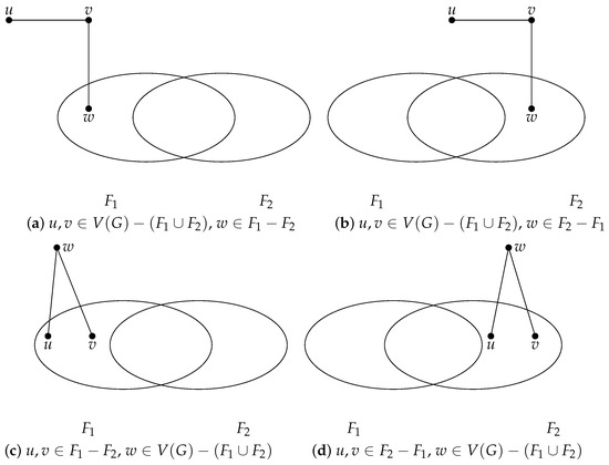Figure 1. Distinguishable pair ($F_1,F_2$) under the MM${}^{*}$ model.

(2) 

There are two vertices $u,v\in F_1-F_2$ and there is a vertex $w\in V\left(G\right)-(F_1\cup F_2)$ such that $(u,w)\in E\left(G\right)$ and $(v,w)\in E\left(G\right)$ (see Figure 1c for an illustration);

(3) 

There are two vertices $u,v\in F_2-F_1$ and there is a vertex $w\in V\left(G\right)-(F_1\cup F_2)$ such that $(u,w)\in E\left(G\right)$ and $(v,w)\in E\left(G\right)$ (see Figure 1d for an illustration).

By the definition of t-diagnosable, similar to Theorem 2, we obtain the following lemma.

Lemma 1.

A graph G is t-diagnosable under the MM${}^{*}$ model if and only if, for any distinct subsets $F_1$ and $F_2$ of $V\left(G\right)$ with $max\{\left|F_1\right|,\left|F_2\right|\}\le t$, $F_1$ and $F_2$ are distinguishable.

The diagnosability of a graph G is upper bounded by its minimum degree.

Theorem 4

([6]). Let G be a graph, then $t\left(G\right)\le \delta \left(G\right)$ under the PMC model and the MM${}^{*}$ model.

2.4. Local Diagnosis

If we only care about the state of some vertices, then Hsu and Tan proposed using the local diagnosis [29] instead of the global diagnosis.

Definition 1

([29]). Let $G=(V,E)$ be a graph and $v\in V$ be a vertex. If given a syndrome ${\sigma }_F$ produced by a faulty vertex set $F\subseteq V$ containing the vertex v with $\left|F\right|\le t$, and every faulty vertex set $F^{\prime }$ compatible with ${\sigma }_F$ and $|F^{\prime }|\le t$ also contains the vertex v, then we say G is locally t-diagnosable at the vertex v.

Definition 2

([29]). Let $G=(V,E)$ be a graph and $v\in V$. The local diagnosability of v, denoted by $t_l\left(v\right)$, is the maximum value of t such that G is locally t-diagnosable at the vertex v.

It is easy to see that $t_l\left(v\right)\le d_G\left(v\right)$ for any vertex $v\in V\left(G\right)$. If $t_l\left(v\right)=d_G\left(v\right)$ for every vertex $v\in V\left(G\right)$, then we say G has a strong local diagnosability property.

Hsu and Tan [29] showed the relation between the diagnosability of a graph G and the local diagnosability of each vertex of the graph as follows.

Theorem 5

([29]). Let G be a graph, then $t\left(G\right)=\min \{t_l\left(v\right)\mid v\in V\left(G\right)\}$.

In [29], the authors provided two sufficient conditions for a vertex to be t-diagnosable under the PMC model. For a vertex x, if there is a Type I structure $T(x;t)$ or a Type II structure $T(x;t-2,2)$ for x, then x is t-diagnosable under the PMC model. See Figure 2 for an illustration. Furthermore, they obtained the following theorem.

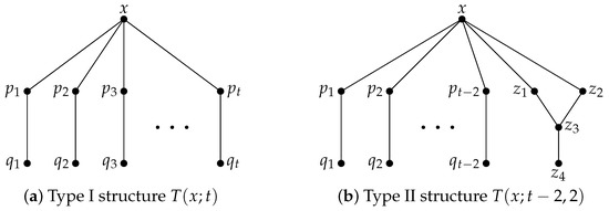
Figure 2. Two local diagnosis structures.

Theorem 6

([29]). Let $G=(V,E)$ be a graph and $x\in V\left(G\right)$ be a vertex. If there is a Type I structure $T(x;d_G\left(x\right))$ or a Type II structure $T(x;d_G\left(x\right)-2,2)$ for x, then $t_l\left(x\right)=d_G\left(x\right)$ under the PMC model.

2.5. The Generalized Cartesian Product of Networks

In this subsection, we generalize the Cartesian product of networks as follows:

Definition 3. 

For $n,m\ge 2$, let $G_1,G_2,\dots ,G_m$ be a set of connected networks each of order n and let H be a connected network of order m. Let $y_1,y_2,\dots ,y_m$ be the vertices of H. The class of the generalized Cartesian product of networks (GCPNs) $G_1,G_2,\dots ,G_m$ with H consists of the following networks. The set of vertices is ${\bigcup }_{i=1}^{m}V\left(G_i\right)$. Each subset $V\left(G_i\right)$ induces a network $G_i$. For each edge $(y_l,y_k)$ of H, we add a perfect matching connecting $V\left(G_l\right)$ to $V\left(G_k\right)$.

Since the perfect matching connecting $G_l$ to $G_k$ is chosen arbitrarily, we have a class of networks. When the matching M is fixed, we obtain a unique network which we denote $\mathbb{G}=G(G_1,G_2,\dots ,G_m;M;H)$.

• When all $G_i$’s are isomorphic to G and M is the canonical perfect matching then $\mathbb{G}=G(G_1,G_2,\dots ,G_m;M;H)$ is the classical Cartesian product of G and H;
• If H is isomorphic to $K_2$, then $\mathbb{G}$ is the Matching Composition Network (MCN), where $K_2$ is the complete network with two vertices;
• If H is isomorphic to $C_m$, then $\mathbb{G}$ is the Cycle Composition Network (CCN), where $C_m$ is the cycle with m vertices;
• We give an example to show that for the same $G_1,G_2,\dots ,G_m$ and H, once the perfect matching is different then we obtain different networks. See Figure 3 for an illustration. In the following, we always use blue lines to represent the edges in $G_i$ and red lines to represent the edges in the perfect matching M.
  

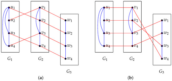  Figure 3. (a) $G(G_1,G_2,G_3;M_1;P_3)$; (b) $G(G_1,G_2,G_3;M_2;P_3)$.

The diagnosability of MCNs and CCNs was considered by Wang et al. in [6]. In this work, we consider H to be any connected graph and $m=\left|V\right(H\left)\right|\ge 3$.

3. The Diagnosability of the GCPNs under the PMC Model

In this section, we consider the local diagnosability of any vertex in $\mathbb{G}$ and obtain the accurate value. By our local diagnosability results, we also determine the diagnosability of $\mathbb{G}$ completely.

Recall that $\left|V\right(H\left)\right|=m$ and $\left|V\right(G_i\left)\right|=n$ for any $i\in \{1,\dots ,m\}$. When $m=2$, Wang et al. investigated the value of $t\left(\mathbb{G}\right)$ in [6]. In this paper, we consider $m\ge 3$ and classify the values of n into two cases: (1) $n\ge 3$, (2) $n=2$.

Theorem 7.

If $m\ge 3$ and $n\ge 3$, then the local diagnosability of each vertex u of $\mathbb{G}$ is equal to its degree $d_{\mathbb{G}}\left(u\right)$ under the PMC model.

Proof. 

For any vertex $u\in V\left(\mathbb{G}\right)$, by Theorem 6, we want to show that there is a Type I structure $T(u;d_{\mathbb{G}}\left(u\right))$ or a Type II structure $T(u;d_{\mathbb{G}}\left(u\right)-2,2)$ for u. Suppose that for $u\in V\left(G_1\right)$, we classify it into two cases.

Case 1. $d_H\left(y_1\right)=1$. Without loss of generality, assume that $N_H\left(y_1\right)=\left\{y_2\right\}$, then $d_H\left(y_2\right)\ge 2$ since $m\ge 3$. Assume that $(y_2,y_3)\in E\left(H\right)$. Let $N_{G_1}\left(u\right)=\{u_1,\dots ,u_k\}$ where $k=d_{G_1}\left(u\right)$. Denote $N_{G_2}\left(u_s\right)$ by $\left\{u_s^{\prime }\right\}$ for $s\in \{1,2,\dots ,k\}$ and denote $N_{G_2}\left(u\right)$ by $\left\{u^{\prime }\right\}$, $N_{G_3}\left(u^{\prime }\right)$ by $\left\{u^{″}\right\}$. Then $T(u;d_{\mathbb{G}}\left(u\right))=(A,B)$ is a Type I structure, where $A=\{u,u_1,\dots ,u_k,u^{\prime },u_1^{\prime },\dots ,u_k^{\prime },u^{″}\},B=\{(u,u_s),(u_s,u_s^{\prime })\mid 1\le s\le k\}\cup \{(u,u^{\prime }),(u^{\prime },u^{″})\}$ and $d_{\mathbb{G}}\left(u\right)=k+1$. See Figure 4 for an illustration.

Figure 4. The Type I structure $T(u;d_{\mathbb{G}}\left(u\right))$ in Case 1 of Theorem 7.

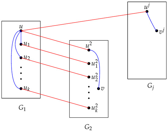
Case 2. $d_H\left(y_1\right)\ge 2$. Assume that $N_H\left(y_1\right)=\{y_2,\dots ,y_l\}$, where $d_H\left(y_1\right)=l-1$ and $l\ge 3$. Let $N_{G_1}\left(u\right)=\{u_1,\dots ,u_k\}$ where $d_{G_1}\left(u\right)=k$. For any $s\in \{1,2,\dots ,k\}$ and $i\in \{2,\dots ,l\}$, denote the neighbor of $u_s$ in $G_i$ by $u_s^i$ and denote the neighbor of u in $G_i$ by $u^i$.

Case 2.1. There exists a vertex $u^i$ such that $N_{G_i}\left(u^i\right)-\{u_1^i,u_2^i,\dots ,u_k^i\}\ne \varnothing$. Without loss of generality, assume that $i=2$ and $v\in N_{G_2}\left(u^2\right)-\{u_1^2,u_2^2,\dots ,u_k^2\}$. For any $j\in \{3,\dots ,l\}$, choose a vertex from $N_{G_j}\left(u^j\right)$ and denote it by $v^j$. Notice that $v^j$ might be one of $u_1^j,u_2^j,\dots ,u_k^j$. Then $T(u;d_{\mathbb{G}}\left(u\right))=(A,B)$ is a Type I structure, where $A=\{u,u_1,\dots ,u_k,u^2,u^3,\dots ,u^l,u_1^2,\dots ,u_k^2,v,v^3,\dots ,v^l\},B=\{(u,u_s),(u_s,u_s^2)\mid 1\le s\le k\}\cup \{(u,u^2),(u^2,v)\}\cup \{(u,u^j),(u^j,v^j)\mid 3\le j\le l\}$ and $d_{\mathbb{G}}\left(u\right)=k+l-1$. See Figure 5 for an illustration.

Figure 5. The Type I structure $T(u;d_{\mathbb{G}}\left(u\right))$ in Case 2.1 of Theorem 7.

Case 2.2. For any $j\in \{2,\dots ,l\}$, $N_{G_j}\left(u^j\right)\subseteq \{u_1^j,u_2^j,\dots ,u_k^j\}$.

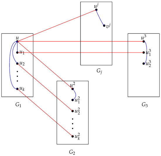
Case 2.2.1. For any $j\in \{2,\cdots ,l\}$, $|N_{G_j}\left(u^j\right)|=1$ and $N_{G_j}\left(u^j\right)=\left\{u_p^j\right\}$ for some $p\in \{1,2,\dots ,k\}$. Without loss of generality, assume that $p=1$. Since $\left|V\right(G_j\left)\right|\ge 3$, $d_{G_2}\left(u^2\right)=1$ and $(u^2,u_1^2)\in E\left(G_2\right)$, so $d_{G_2}\left(u_1^2\right)\ge 2$ and there exists $v\in V\left(G_2\right)-\left\{u^2\right\}$ such that $(v,u_1^2)\in E\left(G_2\right)$. Therefore, $T(u;d_{\mathbb{G}}\left(u\right)-2,2)=(A,B)$ is a Type II structure, where $A=\{u,u_1,u_2\dots ,u_k,u^2,u_1^2,v,u^3,u_1^3,u_2^3,\dots ,u_k^3,u^4,u_1^4,\dots ,u^l,u_1^l\},B=\{(u,u^2),(u,u_1),(u^2,u_1^2),$ $(u_1,u_1^2),(u_1^2,v)\}\cup \{(u,u^3),(u^3,u_1^3),(u,u_s),(u_s,u_s^3)\mid 2\le s\le k\}\cup \{(u,u^j),(u^j,u_1^j)\mid 4\le j\le l\}$, $d_{\mathbb{G}}\left(u\right)=k+l-1$. See Figure 6 for an illustration.

Figure 6. The Type II structure $T(u;d_{\mathbb{G}}\left(u\right))$ in Case 2.2.1 of Theorem 7.

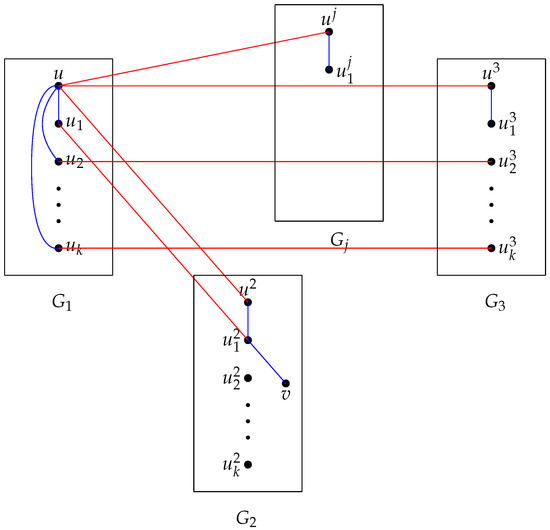
Case 2.2.2. There exist two distinct indices $p,q\in \{1,2,\dots ,k\}$ and two distinct indices $j_1,j_2\in \{2,\dots ,l\}$ such that $u_p^{j_1}\in N_{G_{j_1}}\left(u_p\right)$ and $u_q^{j_2}\in N_{G_{j_2}}\left(u_q\right)$. Assume that $j_1=2$, $j_2=3$ and $p=1,q=2$. For any $j\in \{4,\dots ,l\}$, choose a vertex from $N_{G_j}\left(u^j\right)$ and denote it by $v^j$. Notice that $v^j$ might be one of $u_1^j,u_2^j,\dots ,u_k^j$. Therefore, $T(u;d_{\mathbb{G}}\left(u\right))=(A,B)$ is a Type I structure, where $A=\{u,u_1,\dots ,u_k,u^2,u_1^2,\dots ,u_k^2,u^3,u_1^3,u_2^3,$$u^4,v^4,\dots ,u^l,v^l\},B=\{(u,u_1),(u_1,u_1^3)\}\cup \{(u,u_s),(u_s,u_s^2)\mid 2\le s\le k\}\cup \{(u,u^2),(u^2,u_1^2)\}$$\cup \{(u,u^3),(u^3,u_2^3)\}\cup \{(u,u^j),(u^j,v^j)\mid 4\le j\le l\}$ and $d_{\mathbb{G}}\left(u\right)=k+l-1$. See Figure 7 for an illustration. □

Figure 7. The Type I structure $T(u;d_{\mathbb{G}}\left(u\right))$ in Case 2.2.2 of Theorem 7.

By Theorem 7, we obtain the following result immediately.

Corollary 1. 

If $m\ge 3$ and $n\ge 3$, then $\mathbb{G}$ has the strong local diagnosability property under the PMC model.

The following is a necessary condition for a graph to be locally t-diagnosable at a given vertex.

Proposition 1

([29]). Let $G=(V,E)$ be a graph and $u\in V\left(G\right)$. If G is locally t-diagnosable at the vertex u, then $\left|V\right(G\left)\right|\ge 2t+1$.

Theorem 8.

Let $m\ge 3$, $n=2$. For any vertex $u\in V\left(\mathbb{G}\right)$, if $d_{\mathbb{G}}\left(u\right)\le m-1$ then $t_l\left(u\right)=d_{\mathbb{G}}\left(u\right)$; otherwise, $d_{\mathbb{G}}\left(u\right)=m$ and $t_l\left(u\right)=m-1$.

Proof. 

Since $G_i$ is connected and $\left|V\right(G_i\left)\right|=2$, $G_i\cong K_2$ for any $i\in \{1,\dots ,m\}$. Without loss of generality, suppose that $u\in V\left(G_1\right)$. Assume that $N_H\left(y_1\right)=\{y_2,\dots ,y_l\}$, where $l-1=d_H\left(y_1\right)$. Denote $N_{G_j}\left(u\right)$ by $\left\{u_j\right\}$ and $V\left(G_j\right)-\left\{u_j\right\}$ by $\left\{u_j^{\prime }\right\}$, where $2\le j\le l$. Denote $V\left(G_1\right)-\left\{u\right\}$ by $\left\{u^{\prime }\right\}$. We know that $d_{\mathbb{G}}\left(u\right)=l\le m$, so we distinguish two cases.

Case 1. $d_{\mathbb{G}}\left(u\right)\le m-1$. So, $d_H\left(y_1\right)=l-1\le m-2$ and there exists $y_s\in N_H\left(y_1\right)$ and $y_t\in V\left(H\right)-\{y_1,y_2,\dots ,y_l\}$ such that $(y_s,y_t)\in E\left(H\right)$. Without loss of generality, assume that $s=2$, $t=l+1$ and $N_{G_{l+1}}\left(u_2\right)=\left\{u_{l+1}\right\}$. Then $T(u;d_{\mathbb{G}}\left(u\right))=(A,B)$ is a Type I structure, where $A=\{u,u^{\prime },u_2,u_2^{\prime },\dots ,u_l,u_l^{\prime },u_{l+1}\},B=\{(u,u^{\prime }),(u^{\prime },u_2^{\prime })\}\cup \{(u,u_2),(u_2,u_{l+1})\}\cup \{(u,u_j),(u_j,u_j^{\prime })\mid 3\le j\le l\}$ and $d_{\mathbb{G}}\left(u\right)=l$.

Case 2. $d_{\mathbb{G}}\left(u\right)=m$. By assumption, we have $\left|V\right(\mathbb{G}\left)\right|=2m$. By Proposition 1, we know that u is at most $(m-1)$-diagnosable. Next, we show that u is $(m-1)$-diagnosable. Then $l=m$ and $T(u;m-1)=(A,B)$ is a Type I structure, where $A=\{u,u_2,u_2^{\prime },\dots ,u_l,u_l^{\prime }\},$ $B=\{(u,u_j),(u_j,u_j^{\prime })\mid 2\le j\le l\}$. Therefore, the local diagnosability of u is $m-1$. □

By Theorem 8, we obtain the following result immediately.

Corollary 2. 

If $m\ge 3$, $n=2$ and $\Delta \left(\mathbb{G}\right)\le m-1$, then $\mathbb{G}$ has the strong local diagnosability property under the PMC model.

By Theorems 5, 7 and 8, we obtain the diagnosability of $\mathbb{G}$.

Theorem 9.

If $m\ge 3$ and $n\ge 2$, then the diagnosability of $\mathbb{G}$ under the PMC model is

$$t\left(\mathbb{G}\right)=\left\{\begin{array}{cc}\delta \left(\mathbb{G}\right)-1,\hfill & \mathrm{if}n=2\mathrm{and}H\cong K_m;\hfill \\ \delta \left(\mathbb{G}\right),\hfill & \mathrm{otherwise}.\hfill \end{array}\right.$$

4. The Diagnosability of the GCPNs under the MM${}^{*}$ Model

In this section, we consider the diagnosability of the GCPNs under the MM${}^{*}$ model. When $m=2$, it was considered in [6]. So, we consider $m\ge 3$ in this work.

Lemma 2.

Suppose that $\delta \left(G_i\right)\ge 3$ for any $i\in \{1,2,\dots ,m\}$, where $m\ge 3$. Let $F_1$ and $F_2$ be any two distinct vertex subsets of $V\left(\mathbb{G}\right)$ with $max\left\{\right|F_1|,|F_2\left|\right\}\le \delta \left(\mathbb{G}\right)$. If there is an edge $(u,v)\in M$ such that $u\in F_1\Delta F_2$ and $v\in V\left(\mathbb{G}\right)-(F_1\cup F_2)$, then $F_1$ and $F_2$ are distinguishable under the MM${}^{*}$ model.

Proof. 

By contrast, suppose that $F_1$ and $F_2$ are indistinguishable under the MM${}^{*}$ model. Without loss of generality, we assume that $u\in V\left(G_1\right)\cap (F_1-F_2)$ and $v\in V\left(G_2\right)-(F_1\cup F_2)$. Since $F_1$ and $F_2$ are indistinguishable and $max\left\{\right|F_1|,|F_2\left|\right\}\le \delta \left(\mathbb{G}\right)$, by Theorem 3, we see that $N_{\mathbb{G}}\left(v\right)\subseteq F_1\cup F_2$ and $\delta \left(\mathbb{G}\right)-2\le |N_{\mathbb{G}}\left(v\right)\cap (F_1\cap F_2)|\le \delta \left(\mathbb{G}\right)-1$. We consider the following two cases.

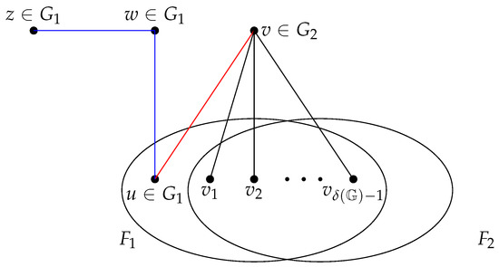
Case 1. $|(F_1\cap F_2)\cap N_{\mathbb{G}}\left(v\right)|=\delta \left(\mathbb{G}\right)-1$. In this situation, we know that $F_1\subseteq N_{\mathbb{G}}\left(v\right)$ and $N_{\mathbb{G}}\left(v\right)\cap V\left(G_1\right)=\left\{u\right\}$. Since $|F_2-F_1|\le 1$ and $d_{G_1}\left(u\right)\ge 3$, there exists $w\in V\left(G_1\right)-(F_1\cup F_2)$ such that $(u,w)\in E\left(G_1\right)$. Since $d_{G_1}\left(w\right)\ge 3$ and $|(F_1\cup F_2)\cap V\left(G_1\right)|\le 2$, there exists $z\in V\left(G_1\right)-(F_1\cup F_2)$ such that $(w,z)\in E\left(G_1\right)$. This contradicts the assumption that $F_1$ and $F_2$ are indistinguishable. See Figure 8 for an illustration.

Figure 8. Illustration of Case 1 in Lemma 2.

Case 2. $|(F_1\cap F_2)\cap N_{\mathbb{G}}\left(v\right)|=\delta \left(\mathbb{G}\right)-2$. Since $F_1$ and $F_2$ are indistinguishable, there exists exactly one vertex x in $F_2-F_1$ such that $(v,x)\in E\left(\mathbb{G}\right)$. We obtain $d_{\mathbb{G}}\left(v\right)=\delta \left(\mathbb{G}\right)$ and $\delta \left(\mathbb{G}\right)-2\le |F_1\cap F_2|\le \delta \left(\mathbb{G}\right)-1$.

Case 2.1. $|F_1\cap F_2|=\delta \left(\mathbb{G}\right)-2$. Then $N_{G_1}\left(u\right)\cap N_{\mathbb{G}}\left(v\right)=\varnothing$ and $|(F_1\cup F_2)-N_{\mathbb{G}}\left(v\right)|\le 2$. Since $d_{G_1}\left(u\right)\ge 3$, there exists $w\in V\left(G_1\right)-(F_1\cup F_2)$ such that $(u,w)\in E\left(G_1\right)$. We know that $N_{\mathbb{G}}\left(v\right)\cap V\left(G_1\right)=\left\{u\right\}$, $N_{\mathbb{G}}\left(v\right)\subseteq F_1\cup F_2$ and $|(F_1\cup F_2)-N_{\mathbb{G}}\left(v\right)|\le 2$, so $|(F_1\cup F_2)\cap V\left(G_1\right)|\le 3$. If $N_{G_1}\left(w\right)\subseteq F_1\cup F_2$, then we obtain $N_{G_1}\left(w\right)\subseteq F_1\Delta F_2$, $|F_1-F_2|=|F_2-F_1|=2$ and $F_1-F_2\subseteq N_{G_1}\left(w\right)$ since $x\notin V\left(G_1\right)$. Let $F_1-F_2=\{u,p\}$, so $(u,w),(p,w)\in E\left(G_1\right)$. This contradicts the assumption that $F_1$ and $F_2$ are indistinguishable. Otherwise, there exists $z\in V\left(G_1\right)-(F_1\cup F_2)$ such that $(w,z)\in E\left(G_1\right)$, which contradicts the assumption that $F_1$ and $F_2$ are indistinguishable.

Case 2.2. $|F_1\cap F_2|=\delta \left(\mathbb{G}\right)-1$. Then $|(F_1\cup F_2)-N_{\mathbb{G}}\left(v\right)|=1$, so $|V\left(G_1\right)\cap (F_1\cup F_2)|\le 2$. There exists $w\in V\left(G_1\right)-(F_1\cup F_2)$ such that $(u,w)\in E\left(G_1\right)$, $z\in V\left(G_1\right)-(F_1\cup F_2)$ such that $(w,z)\in E\left(G_1\right)$. It contradicts to the assumption that $F_1$ and $F_2$ are indistinguishable. □

Next is a result from [6].

Lemma 3

([6]). Suppose that $\delta \left(G\right)\ge 3$. If $F_1$ and $F_2$ are two vertex subsets of G such that $F_1\cap F_2=\varnothing$ and $V\left(G\right)\ne F_1\cup F_2$, then $F_1$ and $F_2$ are distinguishable under the MM${}^{*}$ model.

Theorem 10.

Let $m\ge 3$. If $\delta \left(G_i\right)\ge 3$ for any $i\in \{1,2,\dots ,m\}$, then $t\left(\mathbb{G}\right)\ge \delta \left(\mathbb{G}\right)$ under the MM${}^{*}$ model.

Proof. 

By Theorem 3 and Lemma 1, we need to show that for any two distinct vertex subsets $F_1$ and $F_2$ of $\mathbb{G}$ with $max\left\{\right|F_1|,|F_2\left|\right\}\le \delta \left(\mathbb{G}\right)$, $F_1$ and $F_2$ are distinguishable. By Lemma 3, $F_1$ and $F_2$ are distinguishable if $F_1\cap F_2=\varnothing$ since $\delta \left(\mathbb{G}\right)\ge 4$ and $V\left(\mathbb{G}\right)\ne F_1\cup F_2$. Now, we consider the case that $F_1\cap F_2\ne \varnothing$. By Theorem 9, we know that $t\left(\mathbb{G}\right)=\delta \left(\mathbb{G}\right)$ under the PMC model since $n\ge \delta \left(G_i\right)+1>3$. Thus, there is an edge between $F_1\Delta F_2$ and $V\left(\mathbb{G}\right)-(F_1\cup F_2)$ by Theorem 1. By Lemma 2, $(F_1,F_2)$ is a distinguishable pair if there is an edge $(u,v)\in M$ such that $u\in F_1\Delta F_2$ and $v\in V\left(\mathbb{G}\right)-(F_1\cup F_2)$. Thus, we consider that $N_{\mathbb{G}}\left(u\right)\cap M\subseteq F_1\cup F_2$ for any $u\in F_1\Delta F_2$.

By contrast, suppose that $F_1$ and $F_2$ are indistinguishable under the MM${}^{*}$ model. Let $(p,q)$ be an edge of $\mathbb{G}$ such that $p\in V\left(\mathbb{G}\right)-(F_1\cup F_2)$ and $q\in F_1\Delta F_2$. By assumption, $p,q\in V\left(G_i\right)$ for some $i\in \{1,2,\dots ,m\}$. Without loss of generality, assume that $p,q\in V\left(G_1\right)$ and $q\in F_1-F_2$. Since $F_1$ and $F_2$ are indistinguishable and $max\left\{\right|F_1|,|F_2\left|\right\}\le \delta \left(\mathbb{G}\right)$, by Theorem 3, we see that $N_{\mathbb{G}}\left(p\right)\subseteq F_1\cup F_2$ and $\delta \left(\mathbb{G}\right)-2\le |(F_1\cap F_2)\cap N_{\mathbb{G}}\left(p\right)|\le \delta \left(\mathbb{G}\right)-1$. By assumption, we know that $N_{\mathbb{G}}\left(p\right)\cap V\left(M\right)\subseteq F_1\cap F_2$. Let $p^{\prime }\in N_{\mathbb{G}}\left(p\right)\cap V\left(M\right)$. Without loss of generality, assume that $p^{\prime }\in V\left(G_2\right)$. We classify this into the following two cases.

Case 1. $|F_1\cap F_2|=\delta \left(\mathbb{G}\right)-2$. We know that $\max \left\{\right|F_1-F_2|,|F_2-F_1\left|\right\}\le 2$ and $(F_1\cap F_2)\subset N_{\mathbb{G}}\left(p\right)$. Furthermore, there exists exactly one vertex $x\in F_2-F_1$ such that $(p,x)\in E\left(G_1\right)$. Moreover, $|(F_1\cup F_2)\cap N_{\mathbb{G}}\left(p\right)|=\delta \left(\mathbb{G}\right)$.

Case 1.1. $d_H\left(y_1\right)=1$. Then each vertex of $G_1$ has one neighbor in $G_2$ and $N_{\mathbb{G}}\left(p\right)\cap V\left(M\right)=\left\{p^{\prime }\right\}$. We conclude that $F_1\cap F_2\subset V\left(G_1\right)\cup \left\{p^{\prime }\right\}$. Let $N_{\mathbb{G}}\left(q\right)\cap V\left(M\right)=\left\{q^{\prime }\right\}$ and $N_{\mathbb{G}}\left(x\right)\cap V\left(M\right)=\left\{x^{\prime }\right\}$; by assumption, we obtain $q^{\prime },x^{\prime }\in F_1\Delta F_2$ since $\left|\right\{p^{\prime },q^{\prime },x^{\prime }\left\}\right|=3$ and $p^{\prime },q^{\prime }\in V\left(G_2\right)$. To sum up, we have $F_1\cup F_2\subseteq V\left(G_1\right)\cup V\left(G_2\right)$, $(F_1\cup F_2)\cap V\left(G_2\right)=\{p^{\prime },q^{\prime },x^{\prime }\}$ and $F_1\Delta F_2=\{q,q^{\prime },x,x^{\prime }\}$. Since $d_{G_2}\left(q^{\prime }\right)\ge 3$, there exists $w\in V\left(G_2\right)$ such that $(q^{\prime },w)\in E\left(G_2\right)$. We consider $m\ge 3$, so $d_H\left(y_2\right)\ge 2$. We can find $w^{″}\in V\left(\mathbb{G}\right)-V\left(G_1\right)\cup V\left(G_2\right)$ such that $w^{″}\in V\left(\mathbb{G}\right)-F_1\cup F_2$ and $(w,w^{″})\in M$. This contradicts the assumption that $F_1$ and $F_2$ are indistinguishable.

Case 1.2. $d_H\left(y_1\right)\ge 2$. Let $\{q^{\prime },q^{″}\}\subseteq N_{\mathbb{G}}\left(q\right)\cap V\left(M\right)$ and $\{x^{\prime },x^{″}\}\subseteq N_{\mathbb{G}}\left(x\right)\cap V\left(M\right)$. We know that $N_{\mathbb{G}}\left(x\right)\cap V\left(M\right)$, $N_{\mathbb{G}}\left(q\right)\cap V\left(M\right)$, $N_{\mathbb{G}}\left(p\right)\cap V\left(M\right)$ are mutually disjoint. Notice that $F_1\cap F_2\subseteq V\left(G_1\right)\cup (N_{\mathbb{G}}\left(p\right)\cap V\left(M\right))$. By assumption that $N_{\mathbb{G}}\left(u\right)\cap V\left(M\right)\subseteq F_1\cup F_2$ for any $u\in F_1\Delta F_2$, we have $\{x,x^{\prime },x^{″},q,q^{\prime },q^{″}\}\subseteq F_1\Delta F_2$. This contradicts the assumption that $|F_1\Delta F_2|\le 4$.

Case 2. $|F_1\cap F_2|=\delta \left(\mathbb{G}\right)-1$.

Case 2.1. $d_H\left(y_1\right)=1$. Let $N_{\mathbb{G}}\left(q\right)\cap V\left(M\right)=\left\{q^{\prime }\right\}$. We classify this into two subcases.

Case 2.1.1. $|(F_1\cap F_2)\cap N_{\mathbb{G}}\left(p\right)|=\delta \left(\mathbb{G}\right)-2$. There exists a vertex $x\in F_2-F_1$ such that $(p,x)\in E\left(G_1\right)$. Let $N_{\mathbb{G}}\left(x\right)\cap V\left(M\right)=\left\{x^{\prime }\right\}$. By assumption that $N_{\mathbb{G}}\left(u\right)\cap V\left(M\right)\subseteq F_1\cup F_2$ for any $u\in F_1\Delta F_2$, we have $\{q^{\prime },x^{\prime }\}\subseteq F_1\cup F_2$. On the other hand, $\{q^{\prime },x^{\prime }\}\cap N_{\mathbb{G}}\left(p\right)=\varnothing$ and $|(F_1\cup F_2)-N_{\mathbb{G}}\left(p\right)|=1$, which is a contradiction.

Case 2.1.2. $|(F_1\cap F_2)\cap N_{\mathbb{G}}\left(p\right)|=\delta \left(\mathbb{G}\right)-1$. Since $q^{\prime }\notin N_{\mathbb{G}}\left(p\right)$ and $q^{\prime }\in F_1\cup F_2$, so $F_2-F_1=\left\{q^{\prime }\right\}\subseteq V\left(G_2\right)$. Since $d_{G_2}\left(q^{\prime }\right)\ge 3$ and $(F_1\cup F_2)\cap V\left(G_2\right)=\{p^{\prime },q^{\prime }\}$, there exists $w\in V\left(G_2\right)-(F_1\cup F_2)$ such that $(w,q^{\prime })\in E\left(G_2\right)$. For the same reason, there exists $z\in V\left(G_2\right)-(F_1\cup F_2)$ such that $(w,z)\in E\left(G_1\right)$. This contradicts the assumption that $F_1$ and $F_2$ are indistinguishable.

Case 2.2. $d_H\left(y_1\right)\ge 2$. Let $\{q^{\prime },q^{″}\}\subseteq N_{\mathbb{G}}\left(q\right)\cap V\left(M\right)$. We know that $|F_1\cup F_2|\le \delta \left(\mathbb{G}\right)+1$, $N_{\mathbb{G}}\left(p\right)\subseteq F_1\cup F_2$ and $|N_{\mathbb{G}}\left(p\right)|\ge \delta \left(\mathbb{G}\right)$. By assumption that $N_{\mathbb{G}}\left(u\right)\cap V\left(M\right)\subseteq F_1\cup F_2$ for any $u\in F_1\Delta F_2$, we have $q^{\prime },q^{″}\in F_1\cup F_2$. On the other hand, $\{q^{\prime },q^{″}\}\cap N_{\mathbb{G}}\left(p\right)=\varnothing$ and $|(F_1\cup F_2)-N_{\mathbb{G}}\left(p\right)|\le 1$, which is a contradiction. □

By Theorems 4 and 10, we have the following result.

Theorem 11.

Let $m\ge 3$. If $\delta \left(G_i\right)\ge 3$ for any $i\in \{1,2,\dots ,m\}$, then $t\left(\mathbb{G}\right)=\delta \left(\mathbb{G}\right)$ under the MM${}^{*}$ model.

5. Conclusions

In this work, motivated by the construction of MCNs and CCNs, we propose the definition of the GCPNs. We determine the local diagnosability of each vertex of the GCPNs under the PMC model for $m\ge 3$ and $n\ge 2$. The results show that most of the GCPNs has the strong local diagnosability property under the PMC model. Using our results, we obtain the diagnosability of under the PMC model and the MM${}^{*}$ model for $m\ge 3$ and $n\ge 2$. We include the results of diagnosability of the GCPNs in Table 1. It will be challenging and interesting to consider other types of diagnosability for it, such as conditional diagnosability [3], g-good neighbor conditional diagnosability [30], $t/k$-diagnosability [31] and so on.

Table 1. A summary of diagnosability of the GCPNs.

The Conditions	Diagnosability under the PMC Model	Diagnosability under the MM${}^{*}$ Model
$m=2,n\ge 2$ ([6])	$\left\{\begin{array}{c}n-1,\mathrm{if}{G}_1\cong G_2\cong K_n\hfill \\ \delta \left(\mathbb{G}\right),\mathrm{otherwise}\hfill \end{array}\right.$	$\left\{\begin{array}{c}n-1,\mathrm{if}{G}_1\cong G_2\cong K_n\hfill \\ \delta \left(\mathbb{G}\right),\mathrm{if}{G}_i\ncong K_n\mathrm{for}\mathrm{some}i\mathrm{and}\delta \left(\mathbb{G}\right)\ge 5\hfill \end{array}\right.$
$m\ge 3,H\cong C_m$ ([6])	$\delta \left(\mathbb{G}\right)$, if $\delta \left(G_i\right)\ge 2$ for each $i\in \{1,2,\dots ,m\}$	$\delta \left(\mathbb{G}\right)$, if $\delta \left(G_i\right)\ge 3$ for each $i\in \{1,2,\dots ,m\}$
$m\ge 3,n\ge 2$ (this paper)	$\left\{\begin{array}{c}m-1,\mathrm{if}n=2\mathrm{and}H\cong K_m\hfill \\ \delta \left(\mathbb{G}\right),\mathrm{otherwise}\hfill \end{array}\right.$	$\delta \left(\mathbb{G}\right)$, if $\delta \left(G_i\right)\ge 3$ for each $i\in \{1,2,\dots ,m\}$

References

- Preparata, F.P.; Metze, G.; Chien, R.T. On the connection assignment problem of diagnosable systems. IEEE Trans. Electron. Comput. 1967, 16, 848–854. [Google Scholar] [CrossRef]
- Dahbura, A.T.; Masson, G.M. An O(n2.5) fault identification algorithm for diagnosable systems. IEEE Trans. Comput. 1984, 33, 486–492. [Google Scholar] [CrossRef]
- Lai, P.-L.; Tan, J.J.M.; Chang, C.-P.; Hsu, L.-H. Conditional diagnosability measures for large multiprocessor systems. IEEE Trans. Comput. 2005, 54, 165–175. [Google Scholar]
- Maeng, J.; Malek, M. A comparison connection assignment for diagnosis of multiprocessor systems. In Proceedings of the 11th International Symposium on Fault-Tolerant Computing, Portland, ME, USA, 24–26 June 1981; pp. 173–175. [Google Scholar]
- Sengupta, A.; Dahbura, A.T. On self-diagnosable multiprocessor systems: Diagnosis by the comparison approach. IEEE Trans. Comput. 1992, 41, 1386–1396. [Google Scholar] [CrossRef]
- Wang, Y.; Lin, C.-K.; Li, X.; Zhou, S. Diagnosability for two families of composition networks. Theor. Comput. Sci. 2020, 824–825, 46–56. [Google Scholar] [CrossRef]
- Chiang, C.-F.; Tan, J.J.M. Using node diagnosability to determine t-diagnosability under the comparison diagnosis model. IEEE Trans. Comput. 2009, 58, 251–259. [Google Scholar] [CrossRef]
- Chang, G.-Y.; Chang, G.J.; Chen, G.-H. Diagnosabilities of regular networks. IEEE Trans. Parallel Distrib. Syst. 2005, 16, 314–323. [Google Scholar] [CrossRef]
- Fan, J. Diagnosability of crossed cubes under the two strategies. Chin. J. Comput. 1998, 21, 456–462. [Google Scholar]
- Fan, J. Diagnosability of the Möbius cubes. IEEE Trans. Parallel Distrib. Syst. 1998, 9, 923–928. [Google Scholar]
- Kavianpour, A.; Kim, K.H. Diagnosability of hypercube under the pessimistic one-step diagnosis strategy. IEEE Trans. Comput. 1991, 40, 232–237. [Google Scholar] [CrossRef]
- Cheng, E.; Liptak, L. Diagnosability of Cayley graphs generated by transposition trees with missing edges. Inf. Sci. 2013, 238, 250–252. [Google Scholar] [CrossRef]
- Lee, C.-W.; Hsieh, S.-Y. Diagnosability of two-matching composition networks under the MM* model. IEEE Trans. Dependable Secur. Comput. 2011, 8, 246–255. [Google Scholar]
- Lee, C.-W.; Hsieh, S.-Y. Determining the diagnosability of (1,2)-matching composition networks and its applications. IEEE Trans. Dependable Secur. Comput. 2011, 8, 353–362. [Google Scholar]
- Lin, C.-K.; Teng, Y.-H. The diagnosability of triangle-free graphs. Theor. Comput. Sci. 2014, 530, 58–65. [Google Scholar] [CrossRef]
- Cheng, E.; Liptak, L.; Steffy, D.E. Strong local diagnosability of (n,k)-star graphs and Cayley graphs generated by 2-trees with missing edges. Inf. Process. Lett. 2013, 113, 452–456. [Google Scholar] [CrossRef]
- Ren, Y.; Wang, S. Local diagnosability of bipartite graphs with conditional faulty edges under the Preparata, Metze and Chien’s model. Discret. Appl. Math. 2022, 322, 286–294. [Google Scholar] [CrossRef]
- Chiang, C.-F.; Hsu, G.-H.; Shih, L.-M.; Tan, J.J.M. Diagnosability of star graphs with missing edges. Inf. Sci. 2012, 188, 253–259. [Google Scholar] [CrossRef]
- Wang, D. Diagnosability of enhanced hypercubes. IEEE Trans. Comput. 1994, 43, 1054–1061. [Google Scholar] [CrossRef]
- Armstrong, J.R.; Gray, F.G. Fault diagnosis in a Boolean n-cube array of multiprocessors. IEEE Trans. Comput. 1981, 30, 587–590. [Google Scholar] [CrossRef]
- Saad, Y.; Schultz, M.H. Topological properties of hypercubes. IEEE Trans. Comput. 1988, 37, 867–872. [Google Scholar] [CrossRef]
- Efe, K. The crossed cube architecture for parallel computation. IEEE Trans. Parallel Distrib. Syst. 1992, 3, 513–524. [Google Scholar] [CrossRef]
- Cull, P.; Larson, S. The Möbius cubes. IEEE Trans. Comput. 1995, 44, 647–659. [Google Scholar] [CrossRef]
- Hilbers, P.A.J.; Koopman, M.R.J.; van de Snepscheut, J.L.A. The twisted cube. In Proceedings of the International PARLE Conference on Parallel Architectures and Languages Europe, Eindhoven, The Netherlands, 15–19 June 1987; Volume 258, pp. 152–159. [Google Scholar]
- Dally, W.J. Performance analysis of k-ary n-cube interconnection networks. IEEE Trans. Comput. 1990, 19, 775–785. [Google Scholar] [CrossRef]
- Park, J.-H.; Chwa, K.-Y. Recursive circulant: A new topology for multicomputer networks. In Proceedings of the International Symposium on Parallel Architectures, Algorithms and Networks, ISPAN’94, Kanazawa, Japan, 14–16 December 1994; IEEE Press: New York, NY, USA, 1994; pp. 73–80. [Google Scholar]
- Bondy, J.A.; Murty, U.S.R. Graph Theory; Springer: New York, NY, USA, 2008. [Google Scholar]
- Hsu, L.-H.; Lin, C.-K. Graph Theory and Interconnection Networks; CRC Press: Boca Raton, FL, USA, 2009. [Google Scholar]
- Hsu, G.H.; Tan, J.J.M. A local diagnosability measure for multiprocessor systems. IEEE Trans. Parallel Distrib. Syst. 2007, 18, 598–607. [Google Scholar] [CrossRef]
- Peng, S.-L.; Lin, C.-K.; Tan, J.J.M.; Hsu, L.-H. The g-good-neighbor conditional diagnosability of hypercube under PMC model. Appl. Math. Comput. 2012, 218, 10406–10412. [Google Scholar] [CrossRef]
- Lin, L.; Xu, L.; Zhou, S.; Hsieh, S.-Y. The t/k-diagnosability for regular networks. IEEE Trans. Comput. 2016, 65, 3157–3170. [Google Scholar] [CrossRef]
Disclaimer/Publisher’s Note: The statements, opinions and data contained in all publications are solely those of the individual author(s) and contributor(s) and not of MDPI and/or the editor(s). MDPI and/or the editor(s) disclaim responsibility for any injury to people or property resulting from any ideas, methods, instructions or products referred to in the content. |
© 2023 by the authors. Licensee MDPI, Basel, Switzerland. This article is an open access article distributed under the terms and conditions of the Creative Commons Attribution (CC BY) license (https://creativecommons.org/licenses/by/4.0/).