
Traveling Wave Optical Solutions for the Generalized Fractional Kundu–Mukherjee–Naskar (gFKMN) Model

College of Computer Science, Chengdu University, Chengdu 610106, China
Mathematics 2023, 11(11), 2583; https://doi.org/10.3390/math11112583
Submission received: 11 April 2023
/
Revised: 28 May 2023
/
Accepted: 1 June 2023
/
Published: 5 June 2023
Abstract
:The work considers traveling wave optical solutions for the nonlinear generalized fractional KMN equation. This equation is considered for describing pulse propagation in optical fibers and communication systems using two quite similar approaches, based on the expansion of these solutions in the exponential or polynomial forms. Both approaches belong to the direct solving class of methods for PDEs and suppose the use of an auxiliary equation. The solutions acquired in this paper are obtained from first- and second-order differential equations that act as auxiliary equations. In addition, we generated 3D, contour, and 2D plots to illustrate the characteristics of the obtained soliton solutions. To create these plots, we carefully selected appropriate values for the relevant parameters.
Keywords:
generalized fractional derivative; KMN model; auxiliary equation; exponential expansion; traveling wave optical solutionMSC:
35C071. Introduction
Fractional differential equations (FDEs) have become increasingly important in describing and modeling complex phenomena in various fields of science and engineering. OFDEs, involving fractional derivatives with respect to a single variable, and PFDEs, which involve fractional derivatives with respect to multiple variables, can accurately capture the memory and hereditary properties of the system being modeled. These equations have wide-ranging applications in fields such as physics, chemistry, engineering, biology, finance, and economics, and are particularly useful for describing anomalous diffusion phenomena. Therefore, the study of FDEs is essential for understanding and predicting the behavior of complex systems in many fields of application. However, the non-locality and non-linearity of fractional derivatives present unique challenges in solving and analyzing FDEs. Traditional analytical and numerical methods may not be directly applicable, and new techniques and tools need to be developed to solve and analyze these equations. Despite these challenges, the study of FDEs has led to much important advancement in various fields of science and engineering. The development of new analytical and numerical methods for solving and analyzing FDEs has opened up new avenues for research and has led to a better understanding of complex phenomena. So far, abundant efficient techniques have been proposed for obtaining exact solutions of nonlinear fractional problems such as the generalized projective Riccati equation method [1], the exponential rational function method [2], the sine-Gordon expansion method [3], the auxiliary ordinary differential equation method and the generalized Riccati method [4], the first integral method [5], the Lie symmetry approach [6], the modified Kudryashov method [7], the modified auxiliary equation method [8], the extended exp(−Φ(ξ))-expansion technique [9], the unified method [10], and so on [11,12,13,14].
In the present research, we aim to derive traveling wave solutions to the generalized fractional Kundu–Mukherjee–Naskar (gFKMN) model, which has a dimensionless display as follows [15,16,17,18,19]:
where the quantity is a complex solution to the model and is the complex conjugation of . Moreover, and are two parameters to denote the dispersion term and the nonlinearity term, respectively. This equation is considered for describing pulse propagation in optical fibers and communication systems.
The generalized fractional derivative [20,21] is used here. With a function , the generalized fractional operator of order for is defined as
The generalized fractional derivative satisfies the properties given in the following theorem:
Theorem 1.
Let
, and be
-differentiable at a point
; then:
If, in addition, is differentiable, then
Equation (1) frequently arises in weather science, tidal waves, river and irrigation flows, tsunami prediction, and other applications. Günerhan et al. [22] obtained new exact solutions for Equation (1) using a new extended direct algebraic method. Rizviet al. [23] obtained the singular soliton, dark soliton, combined dark-singular soliton and other hyperbolic solutions for Equation (1) using the csch method, extended tanh–coth method, and extended rational sinh–cosh method. Talarposhti et al. [24] utilized the exp-function method to derive optical soliton solutions for the KMN model under consideration. Onder et al. [25] introduced optical soliton solutions for the KMN equation using the Sardar sub-equation and the new Kudryashov methods. Using the extended Jacobi’s elliptic expansion function and the expa function methods, Zafar et al. [26] obtained novel soliton solutions for the KMN equation. Kumar et al. [27] found dark, bright, periodic U-shaped, and singular soliton solutions for Equation (1) using the generalized Kudryashov and the new auxiliary equation methods. In addition, other authors studied this equation using novel exact solution methods such as the extended trial function method [28], sine-Gordon/sinh-Gordon expansion methods [29], semi-inverse method [30], and Hamiltonian-based algorithm [31].
2. Mathematical Analysis of the Model
To construct new solutions for Equation (1), the following transformations are utilized:
where represents the amplitude portion. We will look for a specific class of traveling wave solutions, which impose the reduction of the PDE (1) to an ODE, by introducing the so-called wave variable:
The phase portion of the solution (3) will be considered to be:
In this model, and denote wave numbers in the x-and y-directions respectively. Moreover, stands for the frequency of the wave and is a constant. Similarly, the parameters and in (4) represent inverse width along the and directions respectively, while is used for the velocity. Inserting (3) along with (4) and (5) into (1), we arrive at two real and imaginary parts, respectively
It will be solved below using two different approaches, both of them based on expansions of the solutions in the form of the given auxiliary equations.
3. Expansion Methods
Let us consider the following fractional NLPDE
Then, if we apply the transformation
on NLPDE (8), it reduces to a nonlinear problem
where is a nonlinear and is an unknown constant to be determined.
In this case, the following general structure will be assumed for the solution of Equation (10):
where the coefficients are unknown parameters. In addition, the number of is calculated by using some balance rules.
Let us consider the first-order differential equation:
Another first-order equation that can be considered an auxiliary equation is:
We will consider below that is an alternative solution of the auxiliary Equation (12), or, respectively, (20), where and are arbitrary constants.
The substitution of (11) into (10) leads to a system of nonlinear equations for and Via symbolic software such as Maple, the solution of the system in terms of and can be determined.
4. Solving Equation (1)
In our specific case of Equation (6), balancing between and gives , both for (12) and for (20). Thus, the following symbolic structure can be considered for the solution of the problem:
4.1. Solutions via First Exponential Expansion
First of all, we insert (27) into (6) and collect all the terms with the same power of . Assuming all coefficients equal to zero, a set of nonlinear equations is derived:
Taking as zero the coefficients of all powers of we obtain a set of polynomial equations in terms of and . In what follows, we outline the solutions for the system obtained using Maple.
Case 1:
Case 2:
Subsequently, utilizing the secured values (20), (30), exact solutions to Equation (1) are obtained.
First, we represent the families of hyperbolic function solutions corresponding to
For Case 1:
For Case 2:
When
where .
The families of periodic function solutions corresponding to are:
For Case 1:
For Case 2:
where .
The families of rational function solutions of type 1, corresponding to are:
For Case 1:
For Case 2:
while that of type 2, corresponding to is:
For Case 2:
4.2. Solutions via Second Exponential Expansion
Again, by substituting (27) into (6) and using (20) recurrently, we obtain a system of algebraic equations and equate the coefficients of to zero as follows:
Equating to zero the coefficients of all powers of yields a set of algebraic equations for and . Solving the system of algebraic equations with the aid of Maple, we obtain
First, we represent the families of hyperbolic function solutions corresponding to
Second, the families of periodic function solutions corresponding to are:
Third, the families of rational function solutions are:
5. Physical Explanation
In this section, we interpret some of the fFKMN model and wave solutions from the perspective of their physical meaning. Through utilization of exponential expansion methods, novel types of traveling wave optical solution were discovered, encompassing hyperbolic, trigonometric, and rational functions. We successfully derived soliton solutions for this nonlinear model, including bright, dark, periodic, singular, and other types of solitons. To gain a comprehensive understanding of their physical behavior, we depicted some of the obtained solutions graphically. The following results were obtained and are presented in the accompanying figures to enhance our understanding of the physical phenomenon at hand. Figure 1, Figure 2 and Figure 3 depict the 3D, contour and 2D plots of the absolute of Figure 1 represents the gFKMN model wave solution given in Equation (31). Figure 1a–c demonstrates that the absolute values of form a dark solitary (peakon soliton) wave solution with the duration when while (red), (green), (blue). Figure 2 depicts the complex wave solution given in Equation (36). We observe from Figure 2a–c that the absolute value of is a singular periodic wave solution with the duration when while (red), (green), (blue). Figure 3 illustrates the complex solitary wave solution given in Equation (45). We observe from Figure 3a–c that the absolute value of is a bright solitary (cuspon soliton) wave solution with the duration when while (red), (green), (blue).
6. Conclusions
In this work, two exponential expansion methods are well applied to the fractional nonlinear KMN model. A generalized fractional derivative is used. As mentioned earlier in the literature section, several researchers have reported diverse methods for obtaining bright, dark, and singular soliton solutions to integer-order KMN models [15,16,17,18,19,20,21,22,23,24,25,26,27,28,29,30,31]. As a result, the researchers focused solely on obtaining bright, dark, and singular soliton solutions for an integer-order KMN model. Compared to the soliton solutions attained in previous studies [15,16,17,18,19,20,21,22,23,24,25,26,27,28,29,30,31], the bright, dark, periodic, and singular soliton wave solutions generated in this study are novel in terms of their use of the generalized fractional derivative. This approach has not been reported in previously published articles, to the best of the authors’ knowledge. The results demonstrate that the employed methods are efficient mathematical techniques to find traveling wave solutions for a fractional NLPDE. Moreover, the studied method can be easily adopted to investigate other fractional NLPDEs arising in mathematics, physics and other applied disciplines.
Funding
This research received no external funding.
Institutional Review Board Statement
Not applicable.
Informed Consent Statement
Not applicable.
Data Availability Statement
Not applicable.
Conflicts of Interest
The authors declare no conflict of interest.
References
- Raza, N.; Osman, M.S.; Abdel-Aty, A.H.; Abdel-Khalek, S.; Besbes, H.R. Optical solitons of space-time fractional Fokas-Lenells equation with two versatile integration architectures. Adv. Differ. Equ. 2020, 2020, 517. [Google Scholar] [CrossRef]
- Ghanbari, B. On novel nondifferentiable exact solutions to local fractional Gardner’s equation using an effective technique. Math. Methods Appl. Sci. 2021, 44, 4673–4685. [Google Scholar] [CrossRef]
- Baskonus, H.M.; Bulut, H.; Sulaiman, T.A. New Complex Hyperbolic Structures to the Lonngren-Wave Equation by Using Sine-Gordon Expansion Method. Appl. Math. Nonlinear Sci. 2019, 4, 129–138. [Google Scholar] [CrossRef] [Green Version]
- Jiong, S. Auxiliary equation method for solving nonlinear partial differential equations. Phys. Lett. A 2003, 309, 387–396. [Google Scholar] [CrossRef]
- Akinyemi, L.; Mirzazadeh, M.; Amin Badri, S.; Hosseini, K. Dynamical solitons for the perturbated Biswas-Milovic equation with Kudryashov’s law of refractive index using the first integral method. J. Mod. Opt. 2022, 69, 172–182. [Google Scholar] [CrossRef]
- Hashemi, M.S.; İnç, M.; Bayram, M. Symmetry properties and exact solutions of the time fractional Kolmogo-rov-Petrovskii-Piskunov equation. Rev. Mex. Fis. 2019, 65, 529–535. [Google Scholar] [CrossRef] [Green Version]
- Hosseini, K.; Ansari, R. New exact solutions of nonlinear conformable time-fractional Boussinesq equations using the modified Kudryashov method. Waves Random Complex Media 2017, 27, 628–636. [Google Scholar] [CrossRef]
- Khater, M.M.; Lu, D.; Attia, R.A. Dispersive long wave of nonlinear fractional Wu-Zhang system via a modified auxiliary equation method. AIP Adv. 2019, 9, 25003. [Google Scholar] [CrossRef] [Green Version]
- Kumar, D.; Kaplan, M. New analytical solutions of (2+1)-dimensional conformable time fractional Zoomeron equation via two distinct techniques. Chin. J. Phys. 2018, 56, 2173–2185. [Google Scholar] [CrossRef]
- Zhang, B.; Zhu, W.; Xia, Y.; Bai, Y. A Unified Analysis of Exact Traveling Wave Solutions for the Fractional-Order and Integer-Order Biswas–Milovic Equation: Via Bifurcation Theory of Dynamical System. Qual. Theory Dyn. Syst. 2020, 19, 11. [Google Scholar] [CrossRef]
- Younas, U.; Ren, J.; Akinyemi, L.; Rezazadeh, H. On the multiple explicit exact solutions to the double-chain DNA dynamical system. Math. Methods Appl. Sci. 2023, 46, 6309–6323. [Google Scholar] [CrossRef]
- Naeem, M.; Rezazadeh, H.; Khammash, A.A.; Shah, R.; Zaland, S. Analysis of the Fuzzy Fractional-Order Solitary Wave Solutions for the KdV Equation in the Sense of Caputo-Fabrizio Derivative. J. Math. 2022, 2022, 3688916. [Google Scholar] [CrossRef]
- Kumar, D.; Yildirim, A.; Kaabar, M.K.A.; Rezazadeh, H.; Samei, M.E. Exploration of some novel solutions to a coupled Schrödinger–KdV equations in the interactions of capillary-gravity waves. Math. Sci. 2022, 1–13. [Google Scholar] [CrossRef]
- Rao, R.; Lin, Z.; Ai, X.; Wu, J. Synchronization of Epidemic Systems with Neumann Boundary Value under Delayed Impulse. Mathematics 2022, 10, 2064. [Google Scholar] [CrossRef]
- Kudryashov, N.A. General solution of traveling wave reduction for the Kundu–Mukherjee–Naskar model. Optik 2019, 186, 22–27. [Google Scholar] [CrossRef]
- Cimpoiasu, R.; Rezazadeh, H.; Florian, D.A.; Ahmad, H.; Nonlaopon, K.; Altanji, M. Symmetry reductions and invariant-group solutions for a two-dimensional Kundu–Mukherjee–Naskar model. Results Phys. 2021, 28, 104583. [Google Scholar] [CrossRef]
- Jhangeer, A.; Seadawy, A.R.; Ali, F.; Ahmed, A. New complex waves of perturbed Shrödinger equation with Kerr law nonlinearity and Kundu-Mukherjee-Naskar equation. Results Phys. 2020, 16, 102816. [Google Scholar] [CrossRef]
- Yıldırım, Y. Optical solitons to Kundu–Mukherjee–Naskar model with trial equation approach. Optik 2019, 183, 1061–1065. [Google Scholar] [CrossRef]
- Bashar, H.; Arafat, S.Y.; Islam, S.R.; Rahman, M. Extraction of some optical solutions to the (2+1)-dimensional Kundu–Mukherjee–Naskar equation by two efficient approaches. Partial Differ. Equ. Appl. Math. 2022, 6, 100404. [Google Scholar] [CrossRef]
- Abu-Shady, M.; Kaabar, M.K. A Generalized Definition of the Fractional Derivative with Applications. Math. Probl. Eng. 2021, 2021, 9444803. [Google Scholar] [CrossRef]
- Martínez, F.; Kaabar, M.K.A. A Novel Theoretical Investigation of the Abu-Shady–Kaabar Fractional Derivative as a Modeling Tool for Science and Engineering. Comput. Math. Methods Med. 2022, 2022, 4119082. [Google Scholar] [CrossRef]
- Günerhan, H.; Khodadad, F.S.; Rezazadeh, H.; Khater, M.M. Exact optical solutions of the (2+1) dimensions Kundu–Mukherjee–Naskar model via the new extended direct algebraic method. Int. J. Mod. Phys. B 2020, 34, 2050225. [Google Scholar] [CrossRef]
- Rizvi, S.T.R.; Afzal, I.; Ali, K. Dark and singular optical solitons for Kundu–Mukherjee–Naskar model. Int. J. Mod. Phys. B 2020, 34, 2050074. [Google Scholar] [CrossRef]
- Talarposhti, R.A.; Jalili, P.; Rezazadeh, H.; Jalili, B.; Ganji, D.D.; Adel, W.; Bekir, A. Optical soliton solutions to the (2+ 1)-dimensional Kundu–Mukherjee–Naskar equation. Int. J. Mod. Phys. B 2020, 34, 2050102. [Google Scholar] [CrossRef]
- Onder, I.; Secer, A.; Ozisik, M.; Bayram, M. On the optical soliton solutions of Kundu–Mukherjee–Naskar equation via two different analytical methods. Optik 2022, 257, 168761. [Google Scholar] [CrossRef]
- Zafar, A.; Raheel, M.; Ali, K.K.; Inc, M.; Qaisar, A. Optical solitons to the Kundu–Mukherjee–Naskar equation in (2+1)-dimensional form via two analytical techniques. J. Laser Appl. 2022, 34, 022024. [Google Scholar] [CrossRef]
- Kumar, D.; Paul, G.C.; Biswas, T.; Seadawy, A.R.; Baowali, R.; Kamal, M.; Rezazadeh, H. Optical solutions to the Kundu-Mukherjee-Naskar equation: Mathematical and graphical analysis with oblique wave propagation. Phys. Scr. 2020, 96, 025218. [Google Scholar] [CrossRef]
- Ekici, M.; Sonmezoglu, A.; Biswas, A.; Belic, M.R. Optical solitons in (2+1)–Dimensions with Kundu–Mukherjee–Naskar equation by extended trial function scheme. Chin. J. Phys. 2019, 57, 72–77. [Google Scholar] [CrossRef]
- Sulaiman, T.A.; Bulut, H. The new extended rational sgeem for construction of optical solitons to the (2+1)–dimensional kundu–mukherjee–naskar model. Appl. Math. Nonlinear Sci. 2019, 4, 513–522. [Google Scholar] [CrossRef] [Green Version]
- He, J.H. Variational principle and periodic solution of the Kundu–Mukherjee–Naskar equation. Results Phys. 2020, 17, 103031. [Google Scholar] [CrossRef]
- Wang, K.-J.; Zhu, H.-W. Periodic wave solution of the Kundu-Mukherjee-Naskar equation in birefringent fibers via the Hamiltonian-based algorithm. EPL Europhysics Lett. 2020, 139, 35002. [Google Scholar] [CrossRef]
- Khater, M.M. Extended Exp (-(ξ))-Expansion Method for Solving the Generalized Hirota-Satsuma Coupled KdV System. Glob. J. Sci. Front. Res. 2015, 15, 1–15. [Google Scholar]
- Harun-Or-Roshid, M.; Rahman, A. The exp (−Φ(η))-expansion method with application in the (1+1)-dimensional classical Boussinesq equations. Results Phys. 2014, 4, 150–155. [Google Scholar] [CrossRef] [Green Version]
- Islam, R.; Alam, M.N.; Hossain, A.K.M.K.S.; Roshid, H.O.; Akbar, M.A. Traveling wave solutions of nonlinear evolution equations via Exp (−Φ(η))-expansion method. Glob. J. Sci. Front. Res. 2013, 13, 63–71. [Google Scholar]
- Akbulut, A.; Kaplan, M.; Tascan, F. The investigation of exact solutions of nonlinear partial differential equations by using exp (− Φ (ξ)) method. Optik 2017, 132, 382–387. [Google Scholar] [CrossRef]
- Rahman, N.; Akter, S.; Roshid, H.O.; Alam, M.N. Traveling wave solutions of the (1+ 1)-dimensional compound KdVB equation by exp (−Φ(η))-expansion method. Glob. J. Sci. Front. Res. 2014, 13, 7–13. [Google Scholar]
- Akbar, M.A.; Ali, N.H.M. Solitary wave solutions of the fourth order Boussinesq equation through the exp (–Φ(η))-expansion method. Springer Plus 2014, 3, 344. [Google Scholar] [CrossRef] [Green Version]
- Hafez, M.G.; Akbar, M.A. An exponential expansion method and its application to the strain wave equation in microstructured solids. Ain Shams Eng. J. 2015, 6, 683–690. [Google Scholar] [CrossRef] [Green Version]
- Hafez, M.G.; Kauser, M.A.; Akter, M.T. Some New Exact Traveling Wave Solutions for the Zhiber-Shabat Equation. Br. J. Math. Comput. Sci. 2014, 4, 2582–2593. [Google Scholar] [CrossRef]
- Hafez, M.; Alam, M.; Akbar, M. Traveling wave solutions for some important coupled nonlinear physical models via the coupled Higgs equation and the Maccari system. J. King Saud Univ.-Sci. 2015, 27, 105–112. [Google Scholar] [CrossRef] [Green Version]
Figure 1.
3D, contour and 2D plots of with and with and .
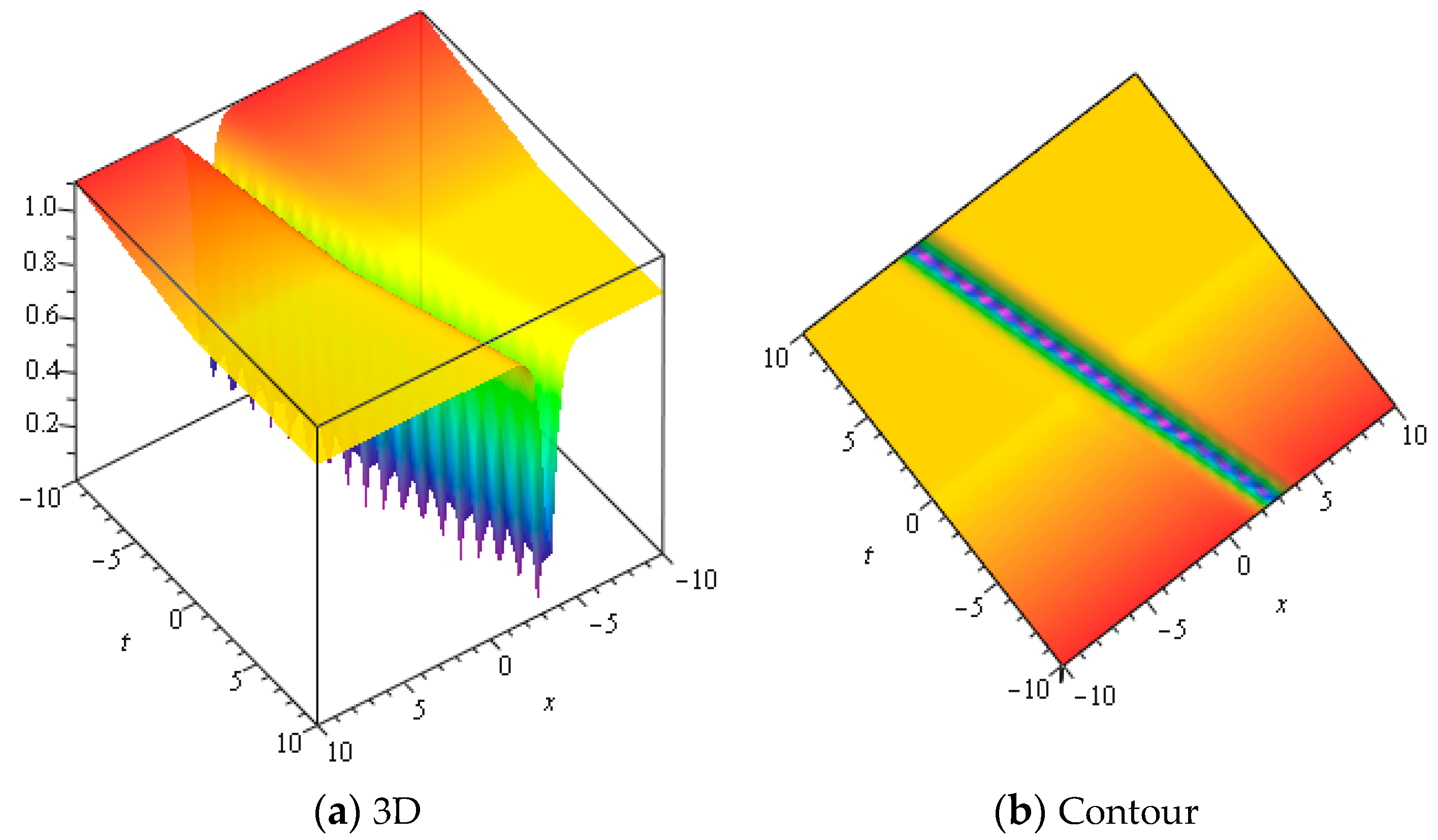
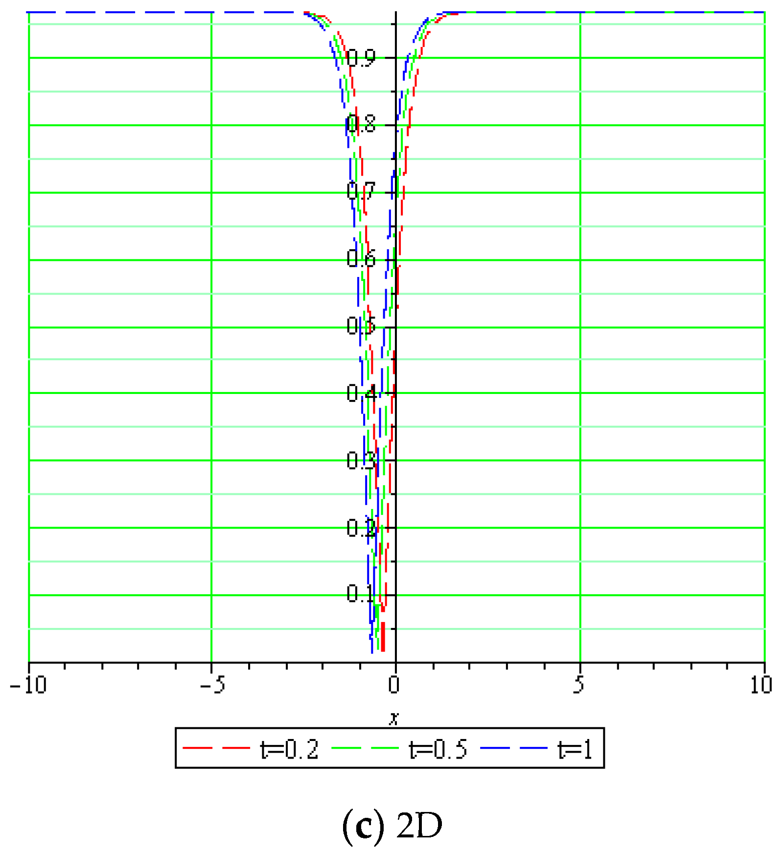
Figure 2.
3D, contour and 2D plots of with and with and .

Figure 3.
3D, contour and 2D plots of with
and with and .
Disclaimer/Publisher’s Note: The statements, opinions and data contained in all publications are solely those of the individual author(s) and contributor(s) and not of MDPI and/or the editor(s). MDPI and/or the editor(s) disclaim responsibility for any injury to people or property resulting from any ideas, methods, instructions or products referred to in the content. |
© 2023 by the author. Licensee MDPI, Basel, Switzerland. This article is an open access article distributed under the terms and conditions of the Creative Commons Attribution (CC BY) license (https://creativecommons.org/licenses/by/4.0/).
Share and Cite
MDPI and ACS Style
Tang, Y. Traveling Wave Optical Solutions for the Generalized Fractional Kundu–Mukherjee–Naskar (gFKMN) Model. Mathematics 2023, 11, 2583. https://doi.org/10.3390/math11112583
AMA Style
Tang Y. Traveling Wave Optical Solutions for the Generalized Fractional Kundu–Mukherjee–Naskar (gFKMN) Model. Mathematics. 2023; 11(11):2583. https://doi.org/10.3390/math11112583
Chicago/Turabian StyleTang, Yong. 2023. "Traveling Wave Optical Solutions for the Generalized Fractional Kundu–Mukherjee–Naskar (gFKMN) Model" Mathematics 11, no. 11: 2583. https://doi.org/10.3390/math11112583
Note that from the first issue of 2016, this journal uses article numbers instead of page numbers. See further details here.