1. Introduction
Next-generation sequencing (NGS) is a massively parallel sequencing technology used to determine the order of nucleotides in entire genomes or targeted regions of deoxyribonucleic acid (DNA) or ribonucleic acid (RNA) which offers ultra-high throughput, scalability, and speed [
1]. With fast development in NGS technology, it becomes more and more widely-used in association studies of genetic variables. Compared with traditional sequencing technologies, such as Sanger technology [
2], NGS technologies can achieve higher sequencing throughput and lower costs. Enormous amounts of NGS data are collected from NGS platforms (for example, MiniSeq, MiSeq, NextSeq 1000 and NovaSeq 6000 from Illumina) by researchers and these researchers own the datasets and conduct genetic studies based on these NGS datasets [
3].
Next-generation sequencing (NGS) data in the format of raw sequencing reads are collected in NGS platforms [
4,
5,
6]. These platforms typically do not provide genotype data. Researchers have proposed multi-step bio-informatics data-processing pipelines to obtain genotypes based on NGS data. A typical pipeline usually includes quality control (QC), alignment of sequences, variant calling, and genotype calling (GC) [
5,
7,
8]. Genotype calling is the process of determining the genotype for each individual and is typically only performed for positions in which a SNP or a ’variant’ has already been called [
9]. After obtaining estimated genotypes, researchers conduct regression analysis to study the relationship between phenotype and genotype, as well as other variables (environmental variables, clinical variables, etc.) [
9,
10,
11].
Regression methods have been used in statistics and bio-statistics including kernel regression [
12], spline smoother [
13], Alternative Conditional Expectations (ACE) [
14], and Additivity Variance Stabilization (AVAS) [
15]. Suppose
and
, and there is a relationship
between
X and
Y via the model
, where the error term
e has zero mean conditional on
X, i.e.,
. Kernel regression can estimate the function
non-parametrically using kernel functions [
12]. The spline smoother estimates the relationship between X and Y, i.e.,
, using splines. That is, the spline smoother assumes that
can be approximated by splines, and then it finds the best spline
m as the (spline estimator) of
[
13]. Alternating conditional expectations (ACE) is a non-parametric method to find the optimal non-linear transformations of the response variable
Y and its predictor variables
X’s to minimize the fraction of variance in transformed
Y not explained by transformed
X’s assuming an additive model. In mathematics, let
be random variables. Suppose
,
,
are zero-mean functions. The fraction of variance in transformed
Y not explained by transformed
X based on additive models are
ACE is a non-parametric method to find optimal transformations (
) to minimize this fraction [
14]. The Additivity Variance Stabilization (AVAS) method is an improved method over ACE which also aimed to find optimal transformation to maximize the fraction in transformed
Y explained by transformed
Xs, and AVAS has better performance than ACE when correlation between transformed
Xs and transformed
Y is small [
15]. An application example of the regression algorithm is arterial volume-weighted arterial spin tagging (AVAST), which is a variant of a pseudo-continuous arterial spin labeling acquisition (PCASL) technique to measure the arterial cerebral blood volume (aCBV) and provides useful information about neuronal activation based on functional magnetic resonance imaging (fMRI) brain data [
16]. Regression methods based on a linear model (LM) and a generalized linear model (GLM) are widely used for association studies. Responses are phenotypes. Genotypes and other variables, including environmental variables and behavior variables, are explanatory variables/predictors. Depending on different types of responses, different regression models can be adopted. For example, bio-statisticians typically conduct logistics regression and linear regression, respectively, for binary responses and continuous responses. If the response is a count/integer type, a Poisson regression can be adopted. To handle complex responses (various types), the framework of a generalized linear model (GLM) can be adopted, which is better than the linear model (LM) framework because LM can only handle continuous responses as we proposed before [
17]. This motivates us to extend our previous linear model framework [
17] to a general linear model framework in this article.
Testing methods are different for common variants and rare variants. Common variants refer to genetic variables with minor allele frequency (MAF) greater than a threshold value
c,
[
18,
19]. Researchers typically set
. Rare variants refer to those with MAF less than
c. For common genetic variants, single-variant testing is conducted in association studies. The genetic effect can be specified by an additive model, dominant model, or recessive model [
9,
20]. Genome-wide association study (GWAS) means to repeat the single-variant testing for all markers genomewide [
9,
20]. For common variants, Chi-square test or F tests are adopted to test for the joint significance of a group of variables. Markers within a gene can be treated as a group and tested simultaneously. Genome-wide gene-based group testing means repeat the single-gene joint-significance testing one-by-one for all genes in the whole genome.
Because rare variants have a small MAF, say
, they have low variations in genotypes so that the power of testing for a variant may not be enough [
18,
21]. Rare-variant testing is often a group test instead of single variable test. There are various testing methods for rare variants in the literature. Among these tests, two big categories are often adopted. Category 1 refers to variable collapsing (VC) testing methods. These methods first calculate one variable based on multiple genetic variants, i.e., collapse/merge multiple variants into one, and then conduct association studies using the calculated variable [
22,
23]. Burden test is a representative method. It conducts association studies between the phenotype and the total number of rare alleles in a group of markers [
23,
24]. Category 2 contains different versions of Sequence Kernel Association testing (SKAT) methods, including SKAT, MK-SKAT, SKAT-O, and BESKAT [
18,
22,
25,
26]. The SKAT method is a representative method in Category 2 and it adopts a linear-model framework (linear regression) to deal with continuous phenotypes, and a logistics-model framework (logistics regression) to deal with binary phenotypes [
26]. Continuous type and binary type are two mostly encountered types of phenotypes in association studies, thus this article focuses on these two types; both categories are genotype-based tests. Genotypes are estimated and association studies are performed between phenotypes and estimated genotypes.
There are estimation errors in genotype calling. Genotype accuracy are influenced by a range of factors, including sequencing errors, alignment accuracy, and sequencing depth. When sequencing depth is low, genotype calling can be very imprecise, which can influence the performance of association methods based on estimated genotypes [
27,
28]. To improve the performance of testing, NGS data-based methods with no genotype calling are recommended. These methods model NGS data directly without genotype calling and have shown better performance [
29,
30].
Researchers have proposed a range of NGS data-based single-variant association testing methods without genotype calling [
29,
30,
31], including our previously proposed UNC combo method [
30]. When sequencing depth is low and genotype calling is not accurate, these NGS data-based single-variant methods can achieve better performance under the scenario of low sequencing depth, heterogeneous sequencing depths, and imprecise genotype calls [
29,
30,
31]; however, there are no NGS data-based group testing methods in the literature except our previously proposed linear model (LM)-based group testing methods [
17]. Being linear model-based, our previously proposed method can only handle continuous phenotypes. However, in the fields of bio-statistics and bio-informatics, especially association studies, other types of phenotypes, especially binary phenotypes (such as disease status and case/control association studies), are widely encountered. It is greatly desired and necessary to extend our methods to enable handling of other types of phenotypes, especially binary phenotypes. Thus, we extend our method from a linear model (LM)-based framework to a generalized linear model (GLM)-based NGS data-based group testing method so that our proposed methods can handle complex responses, including continuous responses (linear regression), binary responses (logistics regression), and count/integer responses (Poisson regression). The proposed NGS-based group testing methods are expected to have an advantage over genotype-based methods, especially when sequencing is low and genotype calling/estimation is not accurate.
Corresponding to genotype-based group testing methods for common variants (joint significance test) and rare variants (variable collapse test) [
22,
26,
32], we fill the literature gap by proposing their corresponding NGS data-based methods without genotype calling. That is, for a group of common variants, the joint significance test (JS) based on NGS data is proposed. For a group of rare variants, the variable collapse test (VC) based on NGS are proposed. Compared with our previous work [
17], the major contribution of this work is that it can handle a range of types of phenotypes, including continuous, binary, and count/integer phenotypes based on the GLM framework, whereas our previous work [
17] can only handle continuous phenotypes based on the LM framework.
In this study, we proposed novel NGS data-based testing methods for association studies based on a generalized linear model (GLM). The proposed methods fill the literature gap as the first NGS data-based group testing methods without genotype calling based on a GLM. We previously used the LM framework to develop association testing methods for a group of genetic variables based on NGS data [
17]; however, our previous methods can only handle continuous responses. In this paper, we aimed to extend our linear model-based framework to a generalized linear model (GLM)-based framework so that our methods can handle other types of responses, especially binary responses, which is commonly-faced in association studies. The objectives of this study were to (1) develop our proposed novel NGS data-based testing methods for association studies based on a theoretical framework of generalized linear models (GLM) and (2) show our proposed methods can achieve better testing performance than their corresponding genotype-based methods.
2. Methodology
Denote the sample size of the study as N. For individual i (), the data are . The term , , and , respectively, represent the phenotype, genotypes, and additional covariates. Examples of additional covariates are environmental variables, gender, and age. The genotype can only have values of 0, 1, or 2 for bi-allelic markers.
Suppose our group testing includes genetic variants. We use a row vector to represent the genotypes for individual i, i.e., where the genotype at variant j for individual i is . We use the row vector represent the intercept and additional covariates, where the value of additional variable j for individual i is denoted as .
Denote genotype matrix with size to be Denote response vector with length n to be Denote the matrix with size for additional covariates to be
2.1. Model Complex Phenotypes Using a GLM Framework
Both the linear model for a quantitative phenotype and the logistic regression model for a binary phenotype conform the framework of the general linear model [
33,
34]. This motivates us to model complex phenotypes by a generalized linear model (GLM) framework. The GLM model-based derivation is a direct extension of our previous linear model (LM)-based framework for testing of a group of variants [
17], which is extended from work on NGS-based single-variant testing [
29].
We model the complex phenotype by a GLM [
33,
34]. For the
i-th individual, the probability of observing phenotype
is modelled to be
where the row vector
and
. The linear predictor is
.
Depending on the type of the phenotype under consideration, different specification of the functions , , and , including
The continuous phenotype, corresponding to a linear regression;
The binary phenotype, corresponding to a logistics regression;
The count (integer) phenotype, corresponding to a Poisson regression.
To be more specific, we show how the modelling of the three types of phenotype belongs to our generalised linear model (GLM) framework. First, consider a continuous phenotype as specified in our previous linear model (LM) framework [
17], i.e.,
, where
. Our previously proposed LM framework is a special case of our GLM framework because
Thus, , , and for a continuous phenotype.
Next, consider a binary phenotype modelled using a logistics regression model, i.e.,
, and
This logistics model is a special case of our GLM framework because
Thus, , and for a binary response.
Thirdly, consider a count (integer) phenotype modelled using a Poisson regression model, i.e.,
, where
. This Poisson regression is also a special case of our GLM framework because
Thus, , and for a count (integer) response.
Our proposed GLM framework is a general framework which can handle different types of responses. The probability of observing phenotype is influenced by predictors ( and ) and parameters . When and are constant functions with respect to , we can drop out and denote the functions as a and . For example, in logistics regression, , , and in Poisson regression, , . The parameters are not involving . Then the probability of observing is influenced by ( and ) and the parameters . In the following, we will discuss two situations, (1) the situation when parameters are ; and (2) the situation when is dropped out, i.e., parameters are .
2.2. Uncertain Genotypes
Because sequencing data and phenotype are conditional independent given true genotypes, we model their joint distribution to be
where
or
depending on whether
can be dropped out, i.e., whether
and
are constant functions with respect to
. For individual
i,
denotes sequencing reads,
denotes the phenotype, and
denotes additional covariates. We denote the genotype state space as
, which contains all possible genotype values for
g. The term
in Equation (
2) refers to sum over all possible values of
g. Because each of the
genetic variants can only has values of 0, 1, and 2,
. The term
is short for the probability of NGS data and genotype, i.e.,
. Here, the estimated allele frequency
is modelled in Skotte et al. [
29]. The log-likelihood function thus can be written as
where
or
depending on whether
is dropped out.
We are interested in testing for genetic effects based on NGS data. The null hypothesis is . Under , we note that the density f does not depends on genotypes so that in the likelihood function under , we can pull it out of the summation.
Then, under
, we simplify the log-likelihood function as follows,
when
is not dropped out and parameters are
. When
is dropped out and the parameters are
, the formula is
Because constrained MLE under can be obtained using the regression of phenotype on additional covariate x (no genotype are used), this motivates us to use score test to develop the methods. Score test only need to know constrained MLE. Note that under , the linear predictor is influenced only by , not by g.
2.3. Joint Significance Test for a Group of Common Genetic Variants
2.3.1. The Situation When Parameters Are
Denote the constrained MLE of the parameters
under
as
. The test statistic is
To calculate this test statistic, we need to evaluate both
(score function) and
(information matrix) at the constrained MLE
. The evaluation of
at the constrained MLE
, i.e.,
is specified in
Appendix C with detailed derivations provided in
Supplementary Material S4 in Supplementary Information File. The evaluation of
at constrained MLE
, i.e.,
is specified in
Appendix D with detailed derivations provided in
Supplementary Material S5 in Supplementary Information File.
Under , . We conducted score test based on testing statistic and p-value of the test can be calculated.
2.3.2. The Situation When Parameters Are
The observed information matrix is
Denote the constrained MLE of the parameters
under
as
. The test statistic is
To calculate this test statistic, we need to evaluate both
and
at the constrained MLE
. The evaluation of
at the constrained MLE
, i.e.,
is specified in
Appendix G with detailed derivations provided in
Supplementary Material S8 in Supplementary Information File. The evaluation of
at the constrained MLE
, i.e.,
is specified in
Appendix H with detailed derivations provided in
Supplementary Material S9 in Supplementary Information File.
Under , the test statistic . We conduct score test based on and calculate p-values.
2.4. Variable Collapse Test for a Group of Rare Variants
2.4.1. The Situation When Parameters Are
For rare variants, variable collapse (VC) methods collapse multiple genetic variables into one variable and use it in testing [
23,
37,
38]. Rare genetic variants can be collapsed in different ways, depending on which method is used. Weighted burden test based on genotypes aggregate/collapse
p rare variants by a weighted sum with the weight
, i.e.,
, where
refers to the genotype for the
j-th rare variants for individual
i. Rare alleles are coded as 0 and wild/reference alleles are coded as 1. The burden test adopts equal weight, i.e.,
. In burden test,
so that association study is performed between the total sum of rare alleles for a group of genetic variants and the phenotype. This means the influence of genotype
on the phenotype is through
.
We model the phenotype using a generalized linear model [
33,
34]. For individual
i, the same generalized linear model is used except the change in linear predictor
. The probability of observing phenotype
is modelled to be
where the row vector
and
is a scalar. The linear predictor in GLM model is
Depending on the type of the responses, we adopt different functions for , , and . Note that aggregates rare genetic variables into one aggregate variable. The probability of observing is influenced by both ( and ) and parameters .
Our model for common variants uses the same GLM framework except the change in linear predictor
, i.e.,
where
. We apply
the chain rule in calculus to derive the formulae for the rare-variant model (Equation (
9)) based on the formulae in the common-variant model, i.e., Equation (
10). The connection between the two models is that the effects of rare variants as modeled by
satisfy the condition that
, where
and
. For burden test which uses equal weight, i.e.,
, so that
is a unit row vector and
[
23,
37]. Then,
. Unequal weights can also be adopted, such as
, where
is the Beta density function. The term
is MAF for the
j-th rare variant [
25,
26,
30].
The same assumption on weights are used in our proposed NGS data-based variable collapse (VC) method. We adopted the assumption of weighted burden test in our test based on NGS data. This assumption has been widely used in VC test based on genotypes in the literature. [
23,
37]. The formula is
, where the weight
is a row vector and
is a scalar. For identification purpose, the constraint
is adopted.
In our joint significance (JS) method for a group of common variants, is modelled as and are parameters and the length of row vector is . In comparison, in our variable collapse (VC) method for a group of rare variants, the linear predictor is modelled as and are parameters and is a scalar. First, under or , the same constrained MLE for and is obtained, no matter which log-likelihood function ( or ) is used. Thus, the same notation is used to represent both the constrained MLE in (note the term 0 refers to a row vector containing elements with all elements equal to 0) and the constrained MLE in (note that the term 0 is a scalar with the value of 0).
The evaluation of the score function at the constrained MLE for the rare-variant model is obtained as follows using the chain rule.
where
is the posterior expectation of the genotype of individual
i given sequencing data
. Evaluation of the last two functions at constrained MLE is 0 because constrained MLE is obtained by constrained optimization of the likelihood function so that the first-order condition is satisfied, i.e., evaluation of the first derivatives are equal to 0.
Working similarly, for rare-variant models, we obtain the observed information matrix, and evaluate it at the constrained MLE. The formulae are
Under , is approximately . Based on the test statistic, we conduct score test and calculate p-value.
2.4.2. The Situation When Parameters Are
Consider the situation when is dropped out and parameters are parameters are . All setups are the same except for the following changes:
The parameters used in rare-variant testing are , where and the parameters in common-variant testing are , where ;
The likelihood functions for rare-variant testing and common-variant testing are, respectively, denoted as and ;
The same notation is used to represent the constrained MLE in (note the term 0 is a scalar of 0) and the constrained MLE in (note the term 0 is a zero row vector of length ).
Evaluation of the score function at the constrained MLE is as follows.
Note that, on the above, the first formula is derived by the chain rule. The second formula is 0 because constrained MLE maximizes the log-likelihood under , so that the first order condition in constrained optimization is satisfied, i.e., evaluation of the first derivatives at constrained MLE is 0.
Working similarly, we derive the observed information matrix, and evaluate it at the constrained MLE. The derivations are as follows.
Under , is approximately . Based on the test statistic, we conduct a score test and calculate the p-value.
2.5. Software to Implement the Methods
We implement our proposed NGS data-based methods using R software (version 4.2.0). We have uploaded the R script files to implement our methods into the Github folder, which is publicly available via the link:
https://github.com/zhengxu0459/NGS.Data.Based.Group.Testing.Based.On.GLM (accessed on 17 May 2023). The Github folder contains six script files to implement our NGS data-based (1) joint significance test and (2) variable collapse test for (i) continuous phenotype, (ii) binary phenotype, and (iii) count phenotype.
2.6. Specification of Simulation Studies
To evaluate the performance of our proposed methods (NGS data-based JS test for common variants and VC test for rare variants) versus literature methods (corresponding methods based on genotypes), we conduct simulation studies. Various setting simulation have been designed.
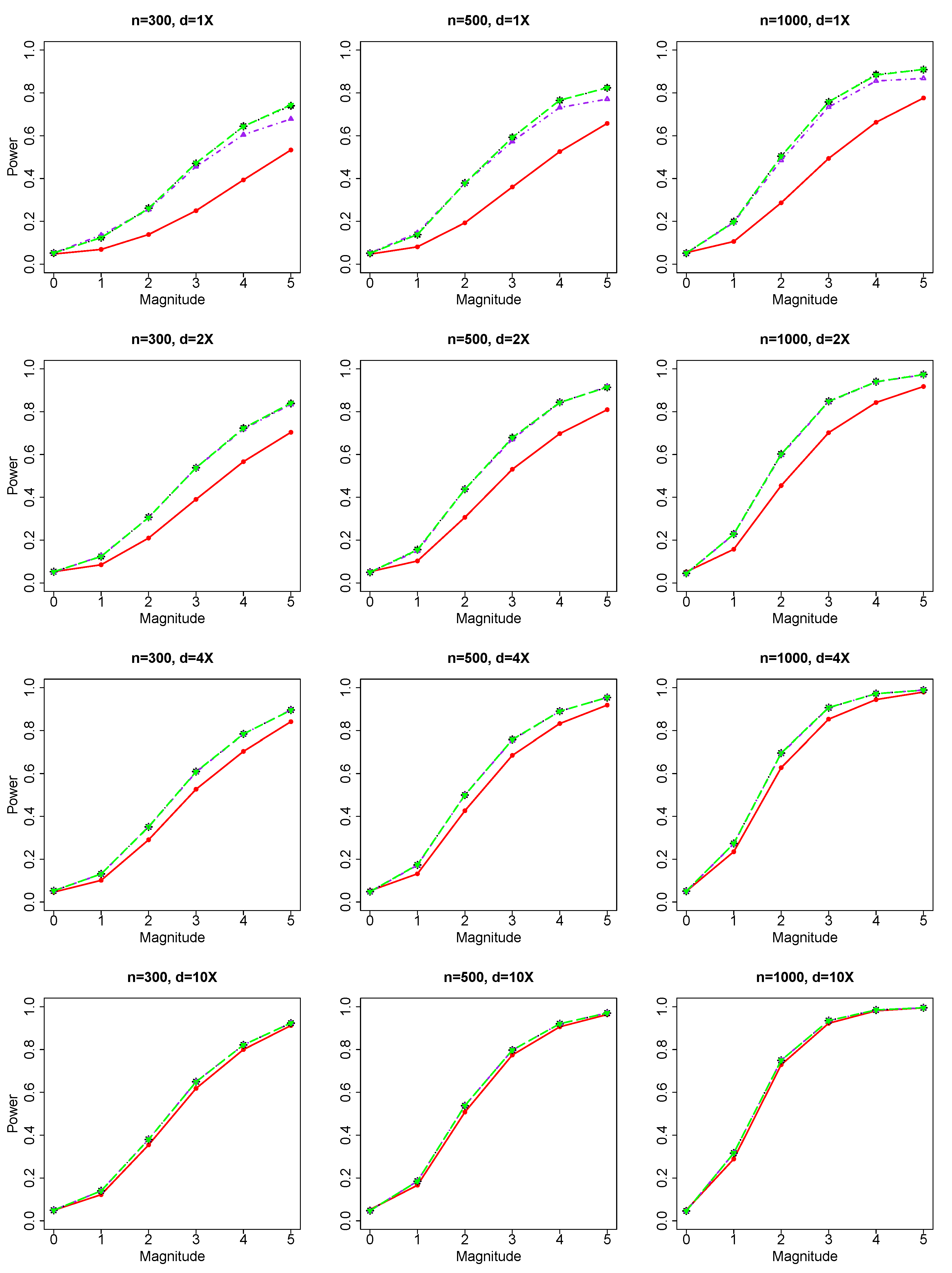
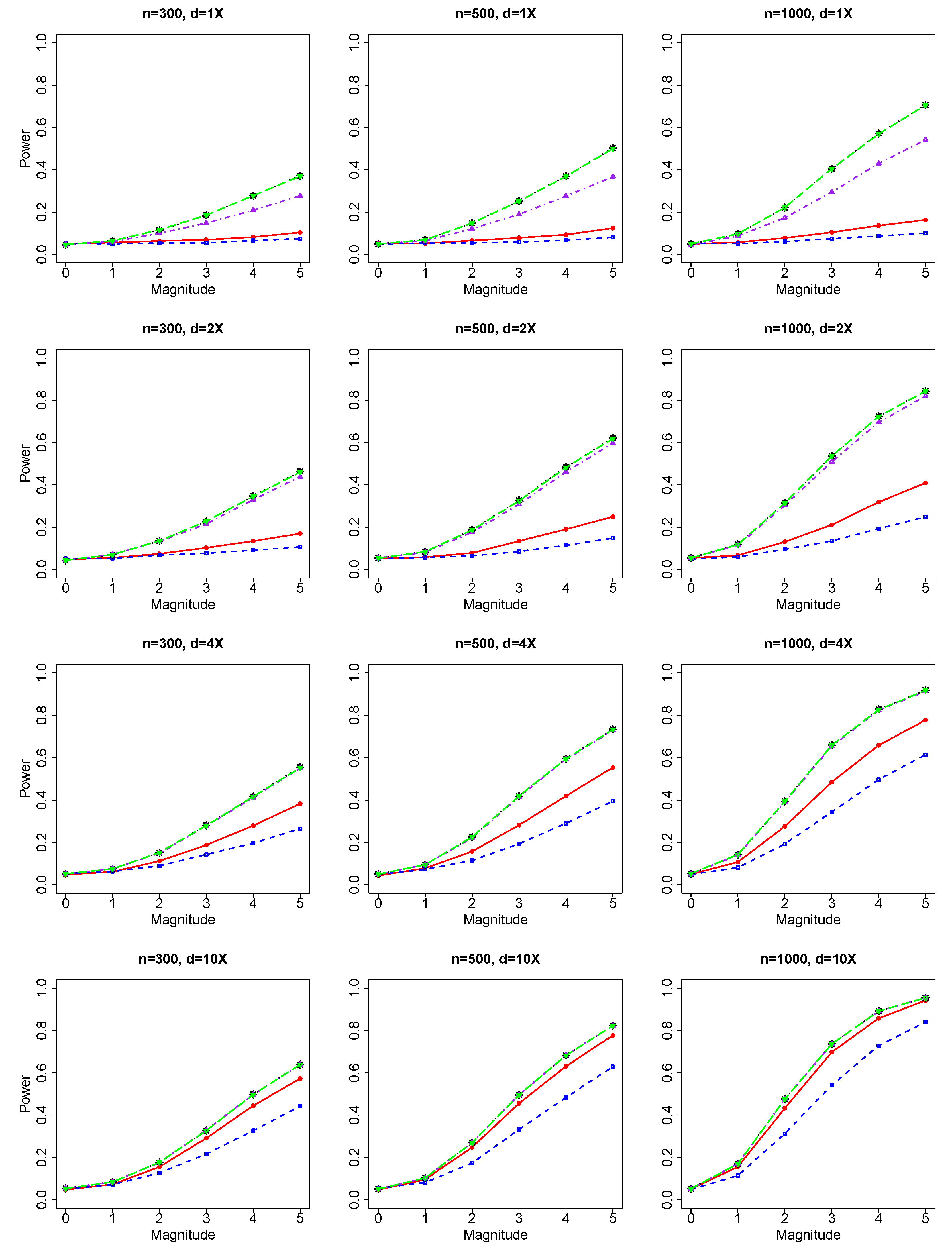
For common genetic variables and binary response, we evaluated the performance of our JS test based on NGS data versus literature methods (Chi-square test) based on genotype. For rare genetic variables and binary response, we evaluated the performance of our VC test based on NGS data versus literature methods (burden test and SKAT test based on genotypes).
We also conducted simulations for count/integer response. Although continuous response and binary response are two of the most commonly encountered types of phenotype in association studies, other types of responses are also in association studies, though not as common as continuous type and binary type. We show that the use of a generalized linear model-framework allows us to handle other types of responses in addition to continuous phenotype. Because genotype-based SKAT testing method is only available for continuous phenotype and binary phenotype [
25], we did not compare our methods with genotype-based SKAT method for count/integer response in rare-variant testing. For count/integer phenotype and rare genetic variables, we evaluated the performance our NGS data-based VC test versus genotype-based burden test literature. For count/integer phenotype and common genetic variables, we evaluated the performance of our NGS data-based JS test versus the genotype-based literature method (Chi-square test).
The software COSI was used to simulate 100 kb genomic regions based on a coalescent model. We adopt the best-fit model in COSI so that regions can be generate to mimic local recombination rate, LD patterns and European population history of Europeans [
39]. We simulate chromosomes in the simulated regions. We used the software ShotGun [
40] to generate sequencing data (per base pair error rate = 0.5%). ShotGun is publicly available at the webpage
https://yunliweb.its.unc.edu/shotgun.html, (accessed on 17 May 2023). We specify various average sequencing depths, such as
. We classify genetic variables as common or rare depending on whether
. Two additional covariates are simulated:
(continuous) and
(binary).
To simulate the binary phenotype, we use the logistics model,
where there are
is genetic variables,
,
,
, and
.
To simulate the count/integer phenotype, we use the Poisson model
where there are
genetic variables,
,
,
, and
.
In simulations of both types, we set genetic effects, i.e., values of , differently in different scenarios, which allows us to evaluate Type I errors and perform power analysis (Type II errors).
Under , we generate 9000 replicates for the evaluation of Type I errors. Type I errors are calculated for all combinations of 3 samples sizes () and 4 sequencing depths (). Results of Type I errors are reported for (1) the JS test of a group of common genetic variables with the binary phenotype and the count/integer phenotype, and (2) the VC test of a group of rare genetic variables with the binary phenotype and the count/integer phenotype.
Then, we conduct simulation studies under the alternative hypothesis , i.e., there are non-zero effects in the genetic variables. In our simulation, we randomly choose multiple genetic variables as causal markers. For common variants, we randomly choose 2 to 5 causal genetic markers. For rare variants, we randomly choose 2 to 10 causal genetic markers. Then we simulate phenotypes based on these causal genetic markers and additional covariates (, ). The total genetic effect is between 0 and 1 (Scale Parameter = 0.2 multiplied by the magnitude range of 0 to 5) with individual genetic effect specified to be the total effect divided by the number of causal variables.
Our simulations have used various (1) sequencing depths, (2) sample sizes, (3) number of causal variables, and (4) genetic effects. Based on simulated data, we evaluate the performance of different testing methods for common variants and rare variants, and compare our NGS data-based methods with the corresponding genotype-based methods in literature.
Our NGS data-based joint significance (JS) test use true allele frequencies (AFs) and two methods to estimate allele frequencies as in Skotte et al. [
29]. NGS data-based JS test 1, 2, and 3, respectively, refer to JS test based on NGS data using (1) true AFs, (2) estimated AFs using the two-step genotype-based method (first estimate genotypes, and then calculate AFs using the estimated genotypes), and (3) one-step MLE estimator of AFs using the likelihood function of NGS data inSkotte et al. [
29]. Both AF estimation methods have been proposed in Skotte et al. [
29]. In general, we expect our testing method based on NGS data to have the best performance when true allele frequencies are used, i.e., our JS test 1 based on NGS data; however, JS Test 1 is not feasible because we do not know true AFs in practice; therefore, we need to use estimated AFs. The use of estimated AFs instead of true AFs is expected to make testing performance a little worse but we expect it will still be better than the corresponding genotype-based methods in the literature. Because one-step MLE of AFs is expected to be more accurate than the two-step genotype-based AF estimator, which has been reported in our previous work based on the same simulated sequencing data [
17]. Thus, we expect our JS Test 3 based on NGS data to be better than our JS Test 2 based on NGS data.
Similarly, Variable Collapse (VC) Test 1, Test 2, and Test 3 based on NGS data refers to VC tests based on NGS data using (1) true AFs, (2) two-step genotype-based estimated AFs, and (3) one-step MLE of AFs. VC Test 1 is an infeasible estimator because, in practice, we do not know true AFs. We expect that VC Test 3 based on NGS data will be better than VC Test 2 based on NGS data.
2.7. Plan of a Real NGS Data Study
We describe our plan to systematically evaluate our methods in real NGS data. To be more specific, in our real NGS data example, we use the recent expansion of the 1000 Genomes Project (1kGP), which includes 602 trios, as described in Byrska-Bishop et al. [
41]. We selected the 1000 Genomes Project (1kGP) for analysis because 1kGP is the largest fully open resource of whole-genome sequencing (WGS) data consented for public distribution without access or use restrictions. Recent expansion of 1kGP has contained 3202 samples, including 602 complete trios, deep sequenced to a depth of 30X, which is a suitable NGS dataset for analysis. The dataset is publicly available at
https://www.internationalgenome.org/data-portal/data-collection/30x-grch38 (accessed on 5 May 2023).
To evaluate the performance of our methods under different scenarios of sequencing depths (
), down-sampling has been conducted to generate sequencing data with depth
and
using the bioinformatics software samtools [
42], accessible at
http://www.htslib.org/ (accessed on 5 May 2023), which can work on NGS data in the bam file format and randomly down-sample NGS reads. For example, if we want to generate NGS data with the depth 10X based on 30X data, we set the down-sample ratio to be 1 out of 3, i.e., the ratio of 1:3. To generate NGS data with sequencing depths
and
, the down-sample ratios are, respectively, 1:30, 1:15, 2:15, and 1:3. Because our methods are for unrelated individuals only, we randomly select at most 1 individual for each family to form a dataset with unrelated individuals. The 1000 genome project has provided accurately-estimated genotypes based on deep sequenced NGS data at
and we use these accurately estimated as true genotypes. The estimated genotypes were obtained by genotype calling on the down-sampled NGS data, i.e., NGS data at depth
and
. Because 1 kGP does not provide phenotype data, we simulate phenotype based on a generalized linear model. Therefore, this real data example makes use of real NGS data and genotype data rather than simulated phenotype data.
In our ongoing project, we will evaluate the performance of our methods and compare with traditional methods in the literature.
4. Discussion
The major finding of our article is that the proposed methods show advantage over their corresponding methods based on genotype in the literature both in testing for a group of common markers and testing for a group of rare markers. The main objective of our study was to apply the GLM framework to derive innovative group testing methods based on NGS data. We fulfil the demand from researchers in bio-statistics, bio-informatics, and biology for developing group testing methods based on NGS data.
Our methods adopt the GLM framework to handle a range of types of phenotypes, including binary responses and continuous responses, which are two mostly encountered types in association studies. Our method extends our previous linear model framework [
17] with the analytical capacity for more complex phenotypes in addition to continuous phenotypes.
In the Results section, we show the findings of comparing our methods with their corresponding methods in the literature for binary phenotype and count phenotype. For continuous phenotype, the GLM-based model will reduce to our previously published LM-based model [
17]. Our findings for group testing of
common variants from binary phenotype and count/integer phenotype are similar to our findings from continuous phenotype for group testing of
common variants published previously [
17]. Similarly, our findings for
rare variants testing from binary phenotype and count/integer phenotype are similar to our findings from
continuous phenotypes for
rare variant testing published previously [
17].
Our proposed model deals with association studies with unrelated/independent individuals. Association studies can be conducted based on related individuals, such as the situation where multiple individuals from the same family are involved in the study. In that case, a generalized linear mixed (GLMM) model instead of a generalized linear (GLM) model is used. Future studies can be on developing testing methods based on NGS data for related individuals. In an ongoing project, we are working to extend our GLM framework to GLMM framework so that it can handle related individuals.
Our proposed methods are based on a score test. We adopt the score test due to its advantage of fast computation and easy derivation of calculation formulae because it only calculates constrained MLE, which is the optimizer maximizing likelihood function under the null hypothesis. The likelihood ratio test can have improved performance compared with the score test [
43,
44]. Future studies can be on developing likelihood ratio-based association tests using NGS data which may have improved performance.
Sequencing depth can impact the comparison of performance between methods based on NGS data and methods based on genotypes. When sequencing depth is big (d = 4X and 10X) and genotype estimation is accurate, methods based on NGS data and methods based on genotypes show similar performance. When sequencing depth is small (depth = 1X and 2X) and genotype estimation is not precise, methods based on NGS data can have better performance than genotype-based methods, which are based on
estimated genotypes [
17,
29,
30]. In practice, given a limited financial budget, low sequencing to include more individuals is preferred to deep sequencing with few individuals sequenced [
29,
30]. Our proposed methods mainly show an advantage when sequencing is low (depth = 1X and 2X).
Our proposed methods are mainly developed based on a theoretical statistical framework of general linear models. We make use of statistical inference methodology to derive the score tests based on the likelihood function of next-generation sequencing (NGS) data and phenotypes with latent/un-observable genotypes. Then we conducted extensive simulation studies to evaluate the performance of our methods and compare our methods with the traditional methods in the theory. In an ongoing project, we are working on systematically evaluating and comparing our methods based on real NGS data. We separate the development of our methods into two stages. In Stage 1, we conduct theoretical development of our methods and simulation studies. In Stage 2, we further evaluate our methods in real NGS data.
We note that simulations performed in our hypothetical scenarios could be biased so that simulation studies could be biased and real data results can provide stronger verification. In our ongoing project, we aimed to systematically evaluate our method in real NGS data.
We note that verification of our methods can be at four levels. The four levels of verification are:
- (1)
Statistically theoretical verification to derive our methods theoretically based on GLM framework to show that our methods are statistically theoretically founded;
- (2)
Simulation studies to evaluate method performance and show that our methods can achieve better performance compared with traditional methods in the literature;
- (3)
Multiple real NGS data examples to evaluate and compare different methods;
- (4)
Biology lab verification and biology literature verification to show our methods indeed find some biologically meaningful genes related to the phenotype.
When possible, we recommend the use of higher levels of verification. For example, simulation studies under a specific scenario can be biased so that real data studies can provide stronger verification. We also recommend the use of as many verification levels as possible to provide verification in different perspectives. The current manuscript provides statistical theoretical derivations and simulation studies. The next steps for verification should be Level 3 (real data verification) and 4 (biology lab verification and biology literature verification). In our ongoing project, we are working on verification from real NGS data. In the future, biology lab verification and biology literature verification can be conducted by collaborating with biology experts.
Future directions of our study include (1) extending our GLM-based methods to generalized linear mixed model (GLMM)-based methods so that they can handle related individuals in association studies; (2) systematically evaluating the performance of our methods and comparing our methods with literature methods in real NGS data; (3) evaluating our methods based on the other three genetic effect models, recessive model, dominant model, and heterogeneous effect models [
45]; and (4) biology lab verification and biology literature verification by collaborating with biology experts.
To describe the effect of genotype (coded as 0, 1, 2) at a single marker on phenotype, four models are widely used. The effect on linear predictor
in the GLM framework is specified differently in the four models [
45], (1) additive model (
); (2) recessive model (
); (3) dominant model (
); and (4) heterogeneous effect model (
). The indicator function
is equal to 1 when the condition is satisfied, and is equal to 0 otherwise. The probability of observing the response in the GLM framework is
and the linear predictor
is modelled differently for the recessive model, dominant model and heterogeneous effect model with
genetic markers. We model linear predictor
in GLM, respectively, as follows,
where the four row vectors (
,
,
,
) have length of
. Although our methods are proposed based on the additive model described in Equation (
10), the methods can be adapted for the other three genetic-effect models (recessive model; dominant model; heterogeneous effect model) by changing
and its first and second derivatives with respect to model parameters.


