1. Introduction
In the last decade, data-driven control has increased its applications in mechanical, electronic, and robotic systems, see, for instance, the works of [
1,
2,
3]. A data-driven approach simplifies the modelling in complex processes using only the online input and output signals of the system. A data-driven model is based on the premise that the system is unknown [
4,
5,
6]. In the same way, the only requirement is the measurable information from the system to approximate its model [
7]. Robot manipulators are considered complex and nonlinear systems with parametric uncertainties. Thus, it is difficult to define their model precisely. The Jacobian matrix represents the system for a kinematic control at the velocity level to achieve the position tasks of the robot’s end-effector. The robot model is obtained through the approximation of the Jacobian matrix using a data-driven approach. In comparison with the traditional robot model, the data-driven modelling requires less information to approximate the Jacobian matrix. The main difference between the traditional and estimation method for robot modelling is the initialization of the Jacobian matrix. While the traditional method has its initial conditions well defined, in the case of a data-driven model, the initial conditions are unknown.
Data-driven modelling works by using the input and output signals from the system [
8,
9,
10]. Therefore, there is no discrimination in the class, structure, or type of robot to apply this approach [
10,
11,
12]. It can be applied to inertial, noninertial, and flexible robots with multi-input and multioutput signals [
13,
14,
15,
16]. The Jacobian matrix is computed only with the measurements of the online joint velocities and end-effector velocities [
17]. Moreover, data-driven modelling and control can be applied to robots as a complement to industrial processes. Ref. [
18] implemented a data-driven model in the joint position control of a robotic arm as single-input single-output (SISO) system. On the other hand, a redundant robot was considered as a discrete-time MIMO system under the principle of a data-driven model, where the time-varying parameter was the estimated Jacobian matrix [
19]. In that particular case, Ref. [
20] proposed the pseudo-Jacobian matrix (PJM) algorithm to estimate the kinematic model of MIMO robotic systems.
Commonly, the computation of a data-driven model in SISO systems is through the principle of the pseudo-partial derivative (PPD) [
21,
22]. Hence, the estimated model starts up with a scalar value. However, the challenge for data-driven models in redundant robots is that they require the Jacobian matrix computation, so that the estimated model requires a set of initial values. The initialization of the Jacobian matrix values represents a challenging topic for data-driven modelling, since the system is unknown even from the beginning. The most common proposal used is to use a zero initialization. Thus, the initial Jacobian matrix values tend to update with the same order of magnitude. However, each value of the Jacobian matrix depends on different orders of magnitude with respect to the robot’s nature. As a consequence, the implementation of the zero-initialization technique diminishes the quality of the estimation algorithm. On the other hand, a Jacobian matrix with random initialization values loses repeatability and estimation performance. The initialization techniques are generally applied to computer vision applications. Ref. [
23] presented the initialization of the segmentation of images for a medical approach. Ref. [
24] implemented the initialization of multimodal pair registration algorithm. However, in the case of the initial values of the Jacobian matrix, it is necessary to satisfy the performance of the robot control. Moreover, it is important to guarantee the convergence of the estimation and control errors. In general, each type of robot demands an exclusive Jacobian matrix of its kinematic model. Therefore, the initialization values for the PJM approach represent a challenge for the topological configuration of each robot. The proposal of this work is to present a generalized methodology to find the adequate values for the Jacobian matrix initialization.
As was mentioned above, the common initialization techniques are selected intuitively by the user’s experience, which are unsatisfactory for starting up the PJM algorithm. This work proposes a novel methodology for the Jacobian initialization based on the kinematic constraints, rank, and domain values of the Jacobian matrix.
This paper establishes a methodology for the initial values’ selection of an estimated Jacobian matrix based on the input and output signals of a redundant robot. The equivalent model is approximated through the PJM algorithm. A control law is also proposed based on a new neuro-fuzzy network that only needs to adapt one parameter to achieve the convergence of the control error. The input to the neuro-fuzzy network is a function in terms of the future error, which avoids the chattering phenomenon [
25].
To demonstrate the initialization methodology, the end-effector control of an eight-degree-of-freedom (dof) redundant robot through three different scenarios is performed, including a regulation control task, trajectory tracking task, and position task against disturbance. Furthermore, a general stability analysis is established, including the parameter settings for the estimation model and the proposed control law.
The structure of this work is as follows:
Section 2 describes the robotic system representation and the Jacobian matrix initialization,
Section 3 introduces the control law design and the Lyapunov analysis,
Section 4 exposes the numerical results, and
Section 5 provides the conclusions.
2. Robotic System Representation
The representation of the end-effector velocity working within the discrete-time domain is approximated by the following expression:
where
is an ideal Jacobian matrix,
is the end-effector velocity,
represents the joints’ velocities, and
is the sampling time.
Assumption 1 below is required for the robot control in a closed-loop configuration.
Assumption 1. The robotic system needs to satisfy the Lipschitz condition, where a positive constant L limits the relationship between the system’s input and output: . This means a change in the output of the system imposes a change in the input of the system.
The ideal Jacobian matrix approach
is represented by:
where
is the Jacobian matrix computed for the PJM algorithm, and
is the estimation error. The Jacobian matrix is the relationship between the output and input signals within the discrete-time domain
where
m is equal to the number of end-effector dofs and
n is equal to the number of dofs of the robot, whereas the robot is considered a MIMO system. The robotic system requires the observability condition in Assumption 2 in order to apply a data-driven model and control.
Assumption 2. To apply a data-driven model and control under the concept of the PJM algorithm, the output of the robotic system needs to be observable, . An approximated Jacobian matrix is computed as a model identification by the measured output (end-effector velocity).
The PJM algorithm approximates the Jacobian matrix, see the reference [
20] for more details. The Jacobian matrix is updated as follows:
where
are the weight parameter and the step parameter, respectively.
2.1. Jacobian Matrix Initialization
The initialization of an estimated model is a critical topic for data-driven modelling and control. The selection of the initial parameters for an estimated Jacobian matrix plays an important role to determine the end-effector trajectory and the convergence time of the control error and the control signals. The first stage of a data-driven model is to determine the initialization values of the Jacobian matrix. Thus, during the second stage, the estimation algorithm approximates the Jacobian matrix. In the first stage, the proposed initialization contains fixed values only to start up the estimation algorithm, and during the second stage the estimation algorithm computes the online Jacobian matrix. The quality of the online estimation algorithm relies on the adequate selection values in the initialization Jacobian matrix. Consequently, the robot can achieve the proper control position task in a closed-loop configuration.
The proposed methodology for the initialization of the Jacobian matrix is presented below.
Assumption 3. The initialization values from the estimated Jacobian matrix and the control signals should satisfy when .
Corollary 1. If the equivalent model obtained by the PJM algorithm fulfils Assumptions 1–3, the initialization of the estimated Jacobian matrix should satisfy the next criteria:
- i
Fulfil the robot kinematic constraints.
- ii
The Jacobian matrix should be full rank, i.e., .
- iii
The domain of the initial Jacobian matrix should guarantee that the estimation error and the control error when .
- iv
The domain of the Jacobian matrix from a discrete-time MIMO system belongs to a domain , and the subdomain from the initial conditions belongs to the Jacobian matrix domain, this means .
- v
Therefore, the error converges to a vicinity of the origin for tracking control in a compact set , when the criteria i to iv are fulfilled.
To exemplify the initialization method, the analysis of this work was applied to a mobile manipulator robot. KUKA youBot has 8 dofs. The estimated Jacobian matrix represents the whole robot with two parts: the omnidirectional platform and the robotic arm. The omnidirectional platform is composed of 3 dofs: 2 prismatic joints in the x and y direction, and 1 revolute joint. The robotic arm is composed of 5 revolute joints. The topology configuration of the robot is .
The structure of the initial estimated Jacobian matrix is defined as:
where
represents the holonomic constraint of the omnidirectional mobile platform expressed as follows
Then,
is the subspace of the estimated Jacobian matrix which represents the minimum change from axis
x with respect to the robotic arm joints represented by
likewise,
is the subspace of the estimated Jacobian matrix which represents the minimum change from axis
y with respect to the robotic arm joints represented by
for this case,
is the subspace of the estimated Jacobian matrix which represents the change from axis
z with respect to the robotic arm. The selection of the
values becomes essential to fulfil the requirements of the estimated Jacobian matrix initialization. It is important to select a domain of values to satisfy the conditions of a full rank of the Jacobian matrix and the convergence of the estimation error regarding the criteria in Assumption 1. The set of values selected were:
Therefore, according to the previous conditions, the initial Jacobian matrix was formed as follows
where the selected values in (
10) satisfied
and they guaranteed an estimation error close to zero, which is demonstrated in Corollary 2.
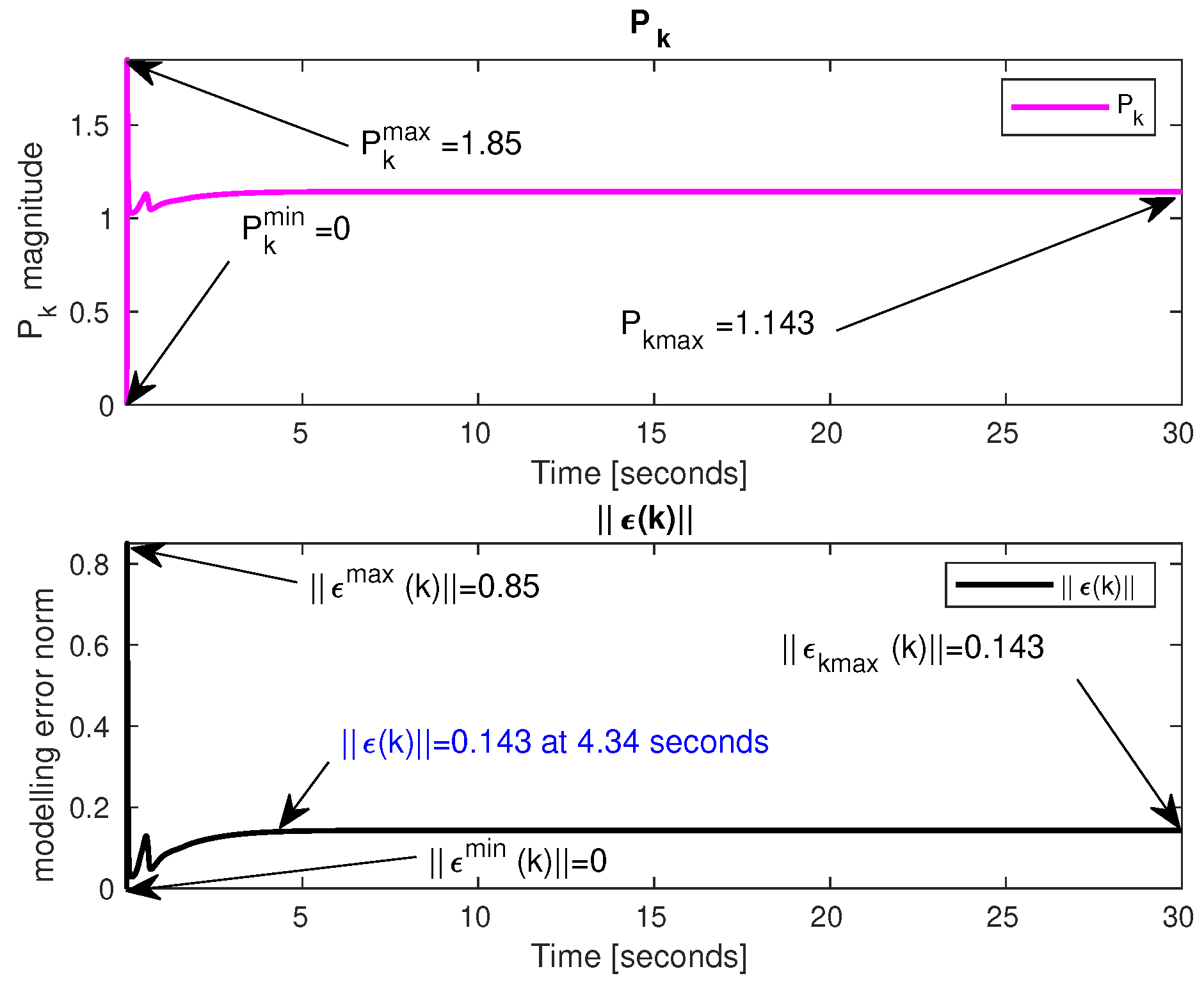
Corollary 2. The term allows a comparison between the ideal Jacobian and the estimated Jacobian . Therefore, it satisfies the next inequality,
Since
and
are the lower and upper values. They depend on the initialization of the Jacobian matrix
[
26];
and
were obtained by simulations using a proportional controller, and
Figure 1 depicts its performance. In terms of the damping factor, the pseudoinverse matrix computation is
where the domain of values is established for
. The PJM algorithm approximates the Jacobian matrix by maintaining the estimation error close to zero. Consequently,
Therefore, an estimation error
is guaranteed, according to
Figure 1, when the selected values in (
10) are applied.
2.2. Equivalent Model Stability Analysis
This section presents the stability analysis for the data-model of the PJM algorithm in (
4) using the Lyapunov candidate function in terms of the estimation error. The estimation error is defined as:
The ideal Jacobian matrix is the reference model; this Jacobian Matrix is computed by the kinematic model considering the Denavit–Hartenberg parameters. Under a classical approach, the robot model requires us to know the physical and mechanical parameters such as the types of joints (revolute or prismatic ones), the link distance, the centre of mass, and the gravity. In contrast, the proposed data-driven model only requires the inputs and outputs to estimate the Jacobian matrix as a model of the robot. For the case where the estimation error achieves to be zero, the updated Jacobian matrix satisfies
; then, the estimated Jacobian matrix becomes:
Hence, the next inequality should be fulfilled
and by substituting (
15) in (
14), the estimation error is
and the change in the estimation error is
Theorem 1. As the KUKA youBot is considered a discrete-time MIMO system, the PJM algorithm can compute an estimated Jacobian matrix, when the system in (3) satisfies the observability and Lipschitz conditions. Therefore, the data-driven model approach is applied when . Proof. The candidate discrete Lyapunov function is
The Lyapunov function change is represented by
The change in the Lyapunov function in terms of the estimation error
is
Substituting (
18) in (
21), it is necessary to look at the Lyapunov stability condition
The Lyapunov conditions are
and
, and the next inequality condition should satisfy
Remark 1.The details of Theorem 1 are discussed in [
27],
the stability analysis of the PJM algorithm and the convergence of the estimation error are relevant for the global stability analysis of a data-driven control in a closed-loop configuration presented below in Theorem 3. Remark 2.The upper and lower joints’ velocities depend on the actuators’ saturation, and mechanical damage in the robot needs to be prevented. Hence, the estimation error must be close to zero.
For
,
, and the stability condition
is accomplished by using (
23). The saturation of the actuators
depends on the robot characteristics (revolute or prismatic joints). Nevertheless, the damages into the KUKA youBot actuators can be prevented under the operating range
. From (
23), the next inequality should satisfy
Accordingly,
, where
is the upper limit, when
, so that (
22) becomes:
Since,
when (
24) is fulfilled and
,
,
i.e., as
. □
3. Control Law
The proposed control law is a proportional controller with adaptive gains for each
ith axis of the robot in the
x,
y, and
z directions. A neuro-fuzzy network was applied to tune the adaptive gains of the controller. The position error of the end-effector is
where
represents the position of the end-effector axis, and
is the desired position task of the robot. The controller design uses the function
in the input of the neuro-fuzzy network in order to improve the tracking of the position error. Hence, the function is defined as:
where
are positive constants. The novelty of the proposed controller is that the function
is the input to the neuro-fuzzy network, and the output of the neuro-fuzzy network tunes the gains of the proportional controller
. The architecture of the adaptive gains is based on the fuzzy rules emulated network (FREN) structure proposed by [
28]. The proposed topology based on a FREN to tune the adaptive gains for the proportional controller is depicted in
Figure 2.
The layers of the FREN are:
Layer 1: The function is defined as the input to the neuro-fuzzy structure.
Layer 2: The second layer contains the linguistic variables as membership functions. The output at the
jth node of this layer is calculated by
as
where
denotes the linguistic variable at the
jth node (
) for the
ith axis. The five linguistic variables are PL for positive large, PS for positive small, ZE for zero, NS for negative small, and NL for negative large.
Layer 3: This layer may be considered as a defuzzification step. In this case, the parameters remain constant.
Layer 4: This is the output of the artificial neuro-fuzzy network, where the gains of the controller are updated for the proportional controller as
where
N is the number of linguistic variables. The output of the FREN,
, contains positive values according to the membership functions taking values between 0 and 1, and positive values for
.
The generalized rules depend on:
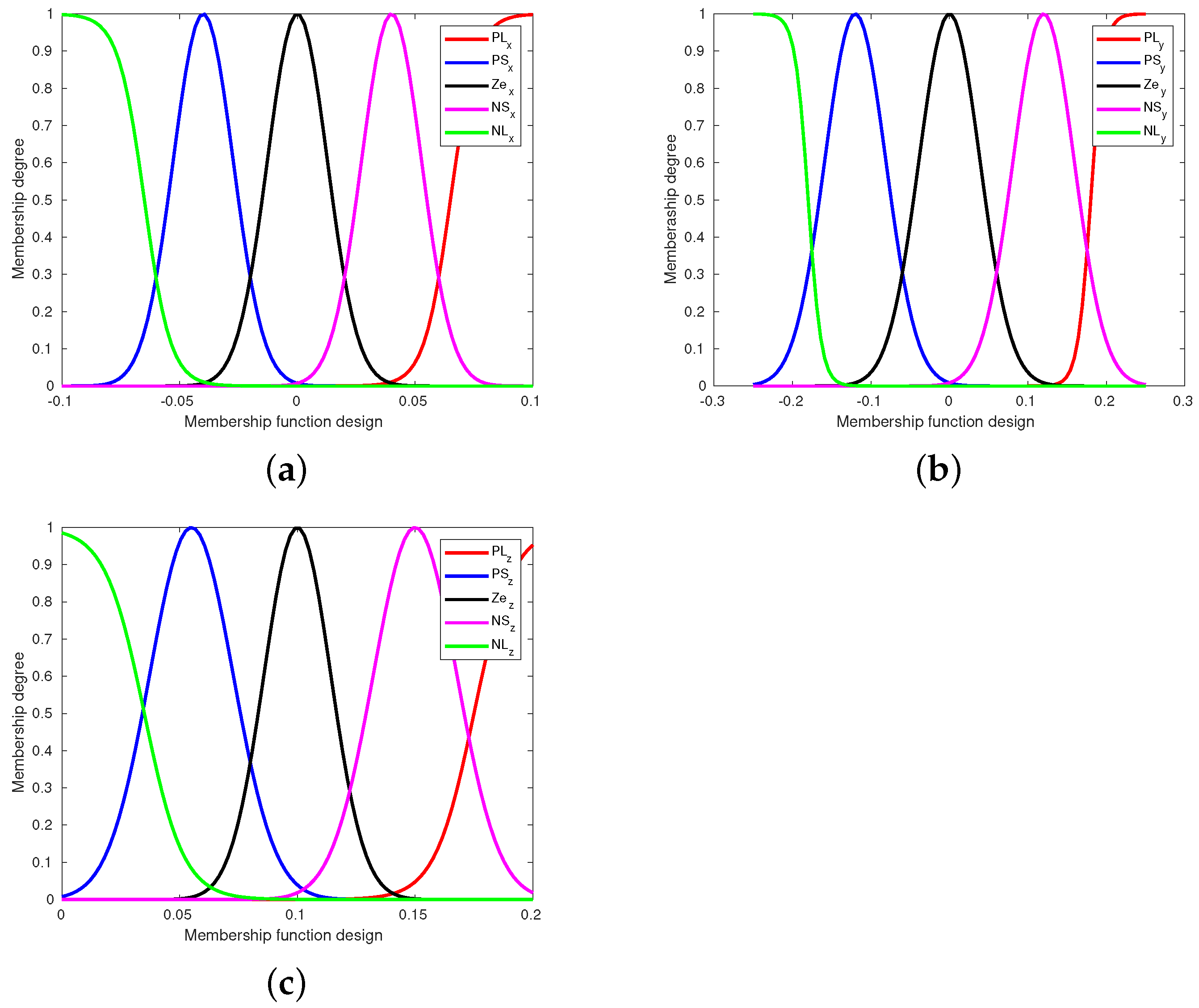
Figure 3a–c show the memberships function for the
x,
y, and
z axes, respectively. The five membership functions were designed by considering the input function to the artificial neuro-fuzzy network
in (27). As the function
was in terms of the position errors, this depended on the physical characteristics of the KUKA youBot, where the omnidirectional platform moved on the
x–
y plane and the robotic arm in the
z direction.
Theorem 2. We can tune the parameters , and in Table 1 through the conditions in (A10). The novelties of the proposed neuro-fuzzy network are:
The five membership functions are designed according to the physical characteristics of the robot axes.
The proposed function is the input of the neuro-fuzzy network. This avoids the chattering action, and it benefits the trajectory tracking control.
The proposed neuro-fuzzy network needs to update only one parameter for each robot axis in order to minimize the control errors.
3.1. Robot Control
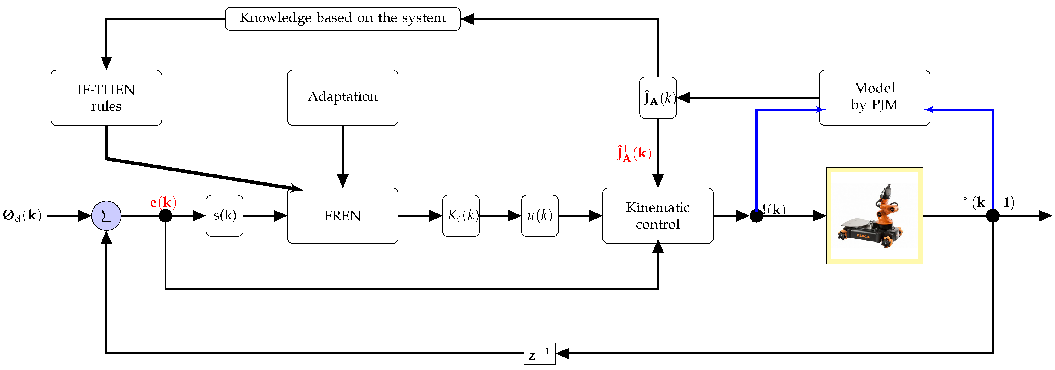
Figure 4 shows the block diagram of the proposed control scheme. The function
is fed with the end-effector position error, which in turn is considered the input to the neuro-fuzzy FREN, where the tuning and adaptation of the gains
is achieved. Later, the gains
, the control error
, and the estimated pseudoinverse Jacobian matrix
are used in the kinematic control law. The equivalent model is derived from the estimation of the Jacobian matrix through the PJM algorithm. By consequence, the loop closes when the end-effector position
reaches the desired position
.
The position error of the end-effector was defined in (
26). Starting from this, the position of the robot’s end-effector is now
where the terms
include the ideal Jacobian matrix and the sampling time, and from (
2), the ideal Jacobian is
. Substituting the current position (
30) in the control error (
26):
The pseudoinverse Jacobian matrix
resolves the inverse kinematics, the joint’s velocities are the control signals
and
contains the control law of
,
, and
as follows
where
is a diagonal matrix which contains the adaptive gains
,
and
. The desired velocity
of the end-effector is included in the tracking control. The next equation solves the pseudoinverse Jacobian matrix
problem
where the value of the damping factor is
. The updated positions are
3.2. Controller Stability Analysis
Theorem 3. For a closed-loop control using the PJM to estimate the Jacobian matrix of a discrete-time MIMO system such as the KUKA youBot, the error position of the end-effector converges to a vicinity of the origin for the trajectory tracking control. When it satisfies the Lipschitz condition, , and .
Proof. The candidate discrete Lyapunov function for a closed-loop control is
for the stability analysis, the Lyapunov condition is
. The change in the Lyapunov function for the controller is
and
are discussed in
Appendix A, and
is the upper-bounded value corresponding to the undefined sign terms in (
A8) and (
A9) within a compact set. Therefore,
, i.e.,
approaches a uniformly ultimately bounded (UUB) system. □
3.3. General Stability Analysis
The aim of this section is to demonstrate the stability analysis through a Lyapunov approach, which involves the dynamic of the estimated model and the control law in a closed-loop configuration. This means the Lyapunov candidate function includes the control and estimation errors.
Theorem 4. Considering that the MIMO system in (3) satisfies the following criteria: Assumption 1: Lipschitz condition.
Assumption 2: observability condition.
Assumption 3: estimation error convergence.
Corollary 1: initialization methodology.
Corollary 2: bounded estimation error value.
Theorem 1: estimation model stability analysis.
Theorem 2: robot control stability analysis.
If Assumptions 1–3, Corollaries 1 and 2, and Theorems 1 and 2 are fulfilled, then the general closed-loop stability of the system is ensured through the model and control Lyapunov functions. The control error converges to a vicinity of the origin and the estimation error approximates zero.
Proof. The stability proof is developed by the general Lyapunov function and its change in the Lyapunov function .
Consider the following general Lyapunov function
considering (
19) and (
36) to propose the general Lyapunov function, where
. The change in the general Lyapunov function is
and substituting (
25) and (
37) in (
39), it is obtained that
This means
when
in
Figure 1, and
, as long as
and
is within a compact set.
The estimation error converges at 4.34 s in
Figure 1; meanwhile, the control error converges at 10 s in
Figure 5b. This means the estimation error should converge before the control error. According to (
30), the control error is in terms of the estimation error. Therefore,
,
and the Lyapunov stability analysis is guaranteed in a vicinity of the origin using (
40). □
4. Results
To start the simulations, it was necessary to consider the initialization conditions mentioned in Corollary 1 and according to the values selected in (
10) for the estimated Jacobian matrix
. The operating values were within
in order to avoid risky damage to the robot structure. The initial values for the prismatic and revolute joints were
and
.
The parameter settings were selected according to Theorems 1–3 in
Table 2.
The performance of the data-driven control was validated by three different simulations.
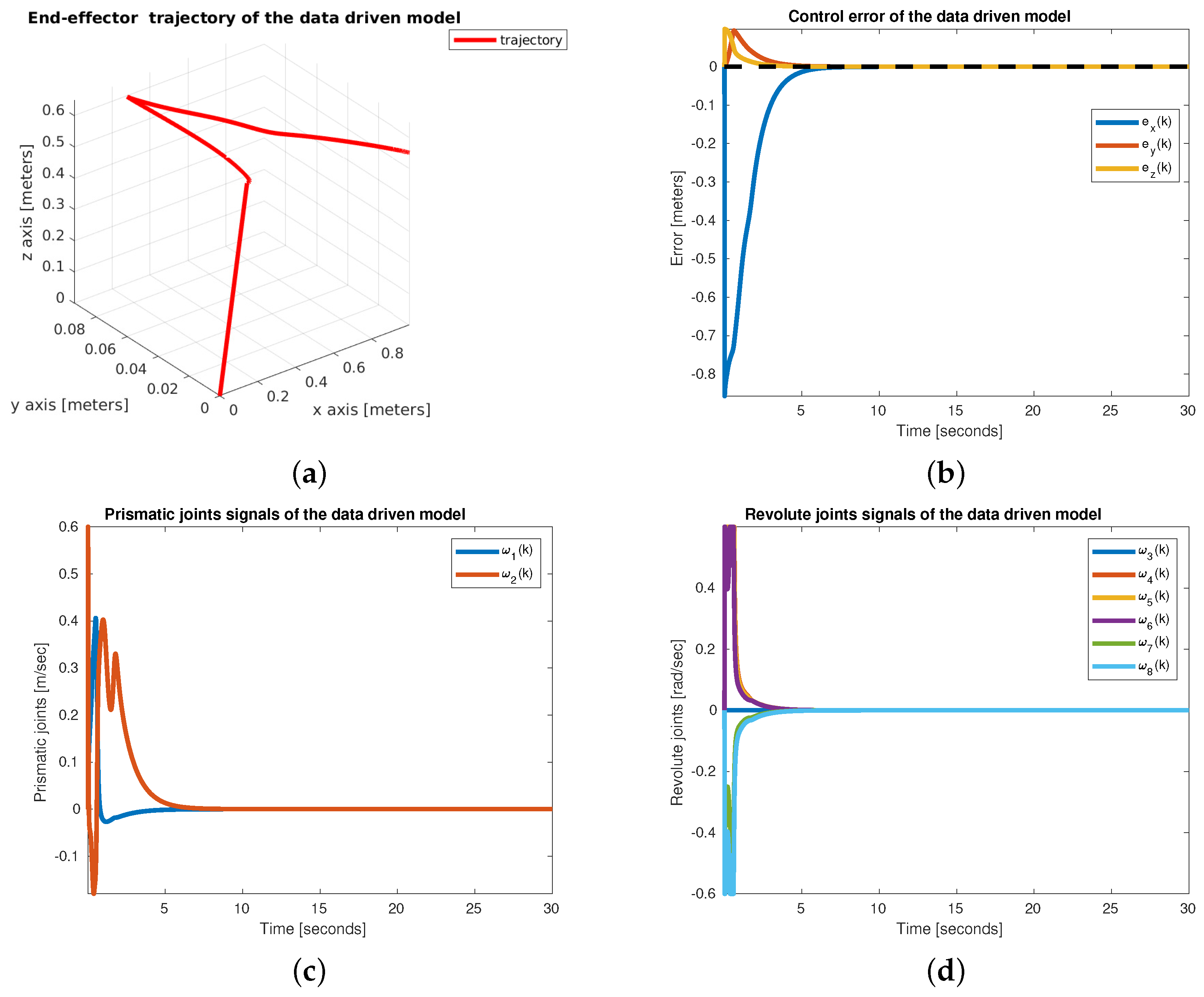
The first simulation was the regulation control of the end-effector. That is, the end-effector reached a fixed desired position.
Figure 5a shows the end-effector for a fixed position task. The convergence of the three position errors are observed in
Figure 5b. The
z-axis position error was the first to converge at 6 s. The
x-axis error converged at 10 s. Finally, the
y-axis error converged at 13 s.
Figure 5c shows the signals of the prismatic velocities
and
; the maximum linear velocity was 0.6
.
Figure 5d depicts the revolute joints’ signals from the robot base and the robotic arm. The maximum angular velocity was 0.6
for
and the minimum velocity was −0.6
, achieved for
.
For the second simulation, while the end-effector reached the object position, a disturbance was applied in the desired position. This means the desired position was changed in order to probe the performance of the robot’s control against disturbances. The trajectory of the end-effector is observed in
Figure 6a, where the change in the trajectory once the objective was moved is clearly observed. The position error is shown in
Figure 6b. It is seen that after 15 s, the disturbance in the end-effector position was introduced, increasing the control errors in the three axes. However, after 20 s, the errors in the three axes converged again. In the case of prismatic joints, it can be seen in
Figure 6c that when applying the disturbance, the maximum linear velocity was 0.6
. On the other hand, the revolute joints reached their minimum and maximum value in ± 0.6
during the disturbance.
In the third simulation, the end-effector followed a circular trajectory.
Figure 7a shows the position of the end-effector on its three axes. The
x and
y axes followed the trajectory, since the
z-axis was maintained constant; in
Figure 7b is shown the position error of the end-effector during tracking control.
Figure 7c depicts the periodic trajectory followed by the prismatic joints in the
x–
y plane.
Figure 7d shows that the revolute joints’ velocities remained close to zero in order to maintain the posture of the robotic arm.
Figure 7e shows the circular trajectory of the end-effector.
The drawback of the proposed initialization method is to be able to identify the four criteria in Corollary 1. It is important to have an understanding of the kinematic constraint, matrix rank, and the stability analysis of the closed-loop control.
5. Conclusions
This work presented a methodology based on a generalized Jacobian matrix initialization applied to a data-driven model approach for a robotic system. A redundant robot is a class of discrete-time MIMO systems. From the data-driven model methods, the system is considered as unknown even from the beginning. The PJM algorithm requires the input–output signals to approximate the Jacobian matrix. Hence, the estimated Jacobian matrix represents the model for a first-order kinematic control in a redundant robot.
The initialization of the Jacobian matrix is an indispensable research topic for data-driven model and control, since the control error and estimation error guarantee their convergence. It was possible to determine the conditions for the initial values of the estimated Jacobian matrix. The conditions were closely tied to the Jacobian matrix rank, the holonomic constraint, the domain of the Jacobian matrix, and the guarantees of control and estimation errors’ convergence. The proposed methodology introduced a specific procedure to identify and select the adequate set of initialization values of the estimated Jacobian matrix by applying a data-driven model in a closed-loop control.
Moreover, de novelty of the proposed proportional controller was the adaptation of its gains using a neuro-fuzzy architecture. The neuro-fuzzy network adapted only one parameter for each end-effector axis; hence, the control errors converged to zero. The control stability analysis included the convergence of the estimation and control errors. Moreover, the conditions of the initial Jacobian matrix, the PJM algorithm, and the proposed robot control were tested in simulations.
As future work, a comparison will be performed between the proposed Jacobian matrix initialization method and an artificial neural network learning approach. Furthermore, the validation of the data-driven modelling and control approach presented in this research will be extended to an experimental setup. Finally, the entire control of the robot pose will be considered, including the position and orientation of the end-effector.


 ,
, 


