Universal Bifurcation Chaos Theory and Its New Applications

Abstract

In this work, an analytical and numerical analysis of the transition to chaos in five nonlinear systems of ordinary and partial differential equations, which are models of autocatalytic chemical processes and interacting populations, is carried out. It is shown analytically and numerically that in all considered systems of equations, further complication of the dynamics of solutions and the transition to chemical and biological turbulence is carried out in full accordance with the universal Feigenbaum-Sharkovsky-Magnitskii bifurcation theory through subharmonic and homoclinic cascades of bifurcations of stable limit cycles. In this case, irregular (chaotic) attractors in all cases are exclusively singular attractors in the sense of the FShM theory. The obtained results once again indicate the wide applicability of the universal bifurcation FShM theory for describing laminar–turbulent transitions to chaotic dynamics in complex nonlinear systems of differential equations and that chaos in the system can be confirmed only by detection of some main cycles or tori in accordance with the universal bifurcation diagram presented in the article.

1. Introduction

It is well known that chaotic dynamics is inherent in almost all natural and social processes and phenomena described by nonlinear systems of ordinary and partial differential equations; however, there was no clear understanding for many years on how there are formed irregular attractors, which differ from stable fixed points, limit cycles and tori. It was thought that there were differences between attractors of autonomous and non-autonomous nonlinear systems of ordinary and partial differential equations and the differential equations with delay arguments. Chaos in Hamiltonian and conservative systems was considered to be essentially different from chaos in dissipative systems. There was also an opinion that irregular attractors of complex nonlinear systems could not be described by systems of differential equations and that a new mathematical apparatus had to be developed to describe them. Additionally, only recently it has been proved and confirmed by numerous examples that irregular (chaotic) attractors can be understood and described within the framework of the theory of bifurcations in nonlinear systems of differential equations. 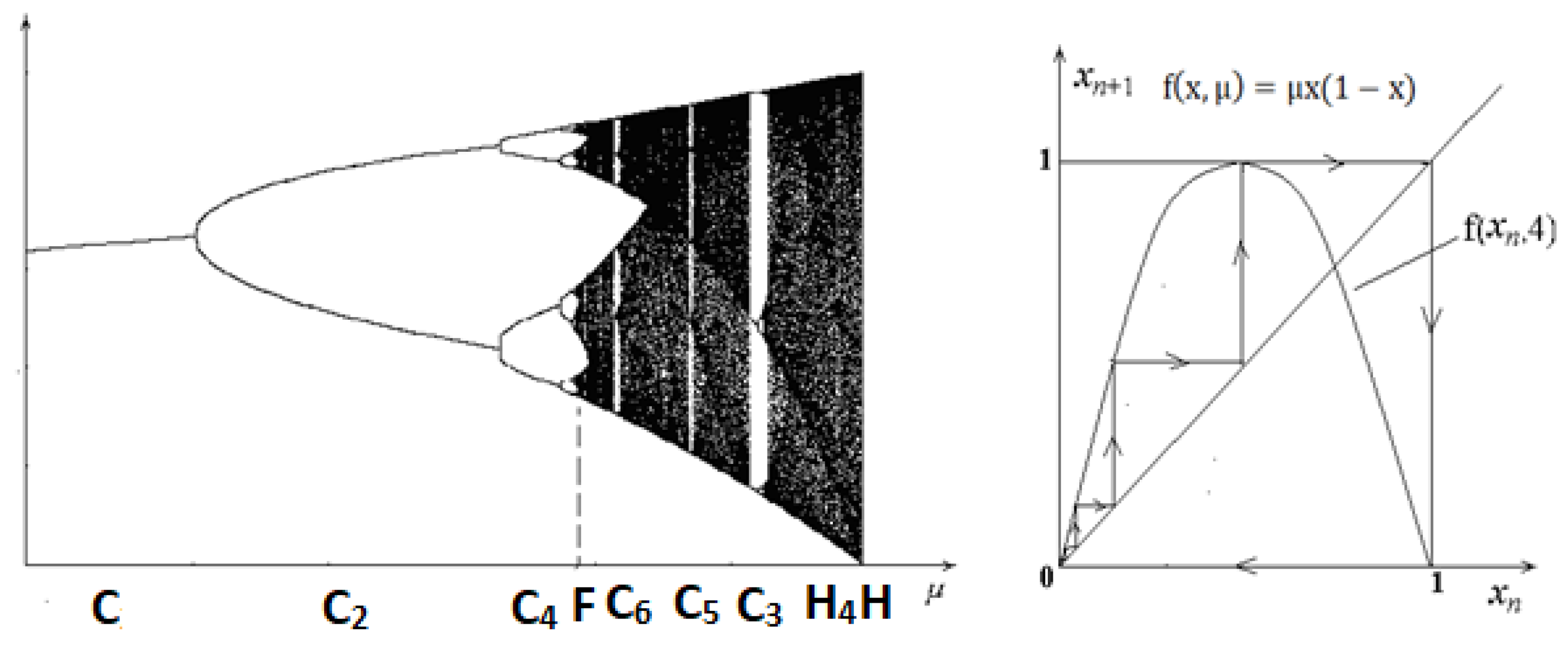It has been proved that there is a universal bifurcation scenario of the transition to dynamical chaos in all kinds of nonlinear systems of differential equations: conservative and dissipative, autonomous and non-autonomous, ordinary, partial and with a delay argument (see [1,2,3]). This is the Feigenbaum–Sharkovsky–Magnitskii (FShM) bifurcation scenario. It begins with the cascade of Feigenbaum period-doubling bifurcations of some stable cycle or torus of arbitrary dimension, and then continues with a cascade of subharmonic Sharkovsky bifurcations of stable cycles or tori of any period up to a cycle or torus of the period three. After that, if possible, the bifurcation scenario continues with a homoclinic or heteroclinic cascade of Magnitskii bifurcations of stable cycles or tori converging to a homoclinic or heteroclinic separatrix contour or toroidal manifold. All irregular (chaotic) attractors that are born during the implementation of such a scenario are only singular attractors, that are non-periodic bounded trajectories in a finite-dimensional or infinite-dimensional phase space, which are the limits of the cycles of the some Feigenbaum cascade and contain an infinite number of unstable periodic trajectories in any of their neighborhoods. The birth of cycles (tori) of the universal bifurcation scenario occurs in accordance with the order

$$2^0⊲2^1⊲2^2⊲\cdots {⊲2}^2·5⊲{\cdots ⊲2}^2·3⊲\cdots ⊲2·5⊲\cdots ⊲2·3⊲\cdots ⊲5⊲\cdots ⊲3⊲\cdots ⊲4⊲\cdots ⊲5⊲··$$

The left part of the order is the Feigenbaum cascade of period-doubling bifurcations of cycle (torus) which ends with the first simplest singular attractor—the Feigenbaum attractor. The middle part of the order is a subharmonic cascade of Sharkovsky bifurcations and ends with the birth of a cycle (torus) of the period three. The right-hand side of the order is a homoclinic cascade of Magnitskii bifurcations and ends in the limit, as a rule, with a homoclinic separatrix loop of the saddle-focus. All cycles (tori) previously born as a result of saddle-node bifurcations become unstable but remain in the system; therefore, if, for example, a stable cycle of period three is found in the system, which ends the subharmonic cascade of bifurcations, then in the system, together with a stable cycle of period three, there exist infinitely many unstable cycles of all periods.

These results were obtained by M. Feigenbaum and A. Sharkovskii for one-dimensional unimodal mappings using the example of a cascade of period-doubling bifurcations and a subharmonic cascade of bifurcations of the logistic mapping [4,5]. The results were further developed by N. Magnitskii, who substantiated the continuation of the subharmonic Sharkovsky cascade by a homoclinic cascade of bifurcations. Then, all the results obtained for one-dimensional unimodal mappings were transferred by N. Magnitskii to non-autonomous two-dimensional dissipative systems of differential equations with periodic coefficients, then to three-dimensional and multidimensional autonomous dissipative systems of ordinary differential equations and partial differential equations, and then to conservative and Hamiltonian systems. The complete universal bifurcation diagram of the universal FShM scenario is presented in Figure 1. The values of the bifurcation parameter are remarked, at which there exist stable main cycles of the cascade: C is an initial cycle, which begins the cascade of Feigenbaum bifurcations; C₂ is the cycle of a double period; C₄ is the cycle of a quadruple period; F is the Feigenbaum attractor; C₆ is the cycle of period six in the cascade of Sharkovsky bifurcations; C₅ is the cycle of period five; C₃ is the cycle of period three, which ends the cascade of Sharkovsky bifurcations; H₄ is the homoclinic cycle of period four, H is the homoclinic separatrix contour (separatrix loop). Note that the cycles of periods two and three of the subharmonic cascade are also cycles of the same periods of the homoclinic cascade of bifurcations. On the right in Figure 1, the separatrix loop for logistic mapping is shown.

If a system of equations is strongly dissipative, then, as a rule, a complete cascade of Sharkovsky bifurcations and a complete (or incomplete) homoclinic cascade of bifurcations are realized in the system. For systems with weak dissipation, the cycles of the right part of the FShM order may not be born, and the cascade of bifurcations may end before reaching the cycle of period three. For conservative and Hamiltonian systems, only an incomplete cascade of Feigenbaum bifurcations is usually realized with the birth of elliptic tori around the cycles of the cascade.

It is proved in papers by this author and in other papers that the FShM bifurcation scenario of transition to dynamical chaos is realized in classical dissipative two-dimensional non-autonomous systems with periodic coefficients, such as as Mathieu, Croquette and Duffing–Holmes systems, and in three-dimensional dissipative autonomous systems, such as Lorenz, Chua, Sprott, Ressler, Chen, Rabinovich–Fabricant, Vallis, Magnitskii, Anishchenko–Astakhov, Volterra–Gause, Pikovskii–Rabinovich–Trakhtengertz, Sviregev, Rucklidge, Genezio–Tesi, Wiedlich–Trubetskov systems [1,2,3,6,7,8,9,10,11], and many others. This scenario of transition to chaos also takes place in many and infinitely dimensional systems of nonlinear ordinary differential equations, such as Rikitaki system, Lorenz complex five-dimensional system, Mackey–Glass equation with delay argument [1,2,3], and many others. This scenario of transition to chaos takes place also in many partial differential equations and systems, such as Brusselator and Kuramoto–Tsuzuki (time dependent Ginzburg–Landau) equations, reaction–diffusion and FitzHugh–Nagumo type systems of equations, nonlinear Schrodinger and Kuramoto–Sivashinskii equations [1,2,3,12,13,14], and others. Moreover, this scenario also describes the laminar–turbulent transitions in any tasks for Navier–Stokes equations and transition to chaos in Hamiltonian and conservative systems, such as conservative Croquette and Duffing–Holmes equations, Mathieu–Magnitskii and Yang–Mills–Higgs Hamiltonian systems [2,3,15,16,17,18,19,20,21,22], and others. The listed systems of equations describe a variety of complex natural, social, scientific and technical processes and phenomena in physics, chemistry, biology, economics, medicine and sociology, which emphasizes the universal applicability of the considered bifurcation approach.

However, many works continue to appear in the scientific literature, in which the authors, not understanding the essence of the ongoing processes, present new attractors allegedly discovered by them in nonlinear systems of differential equations. “Hidden” attractors for systems with stable singular points or no singular points at all are explained by the authors by the presence of the Smale’s horseshoe or by the found numerically positive Lyapunov exponent, or by the so-called “intermittency”. Hyperchaos in the system is explained by the numerically found two positive Lyapunov exponents. Spatio-temporal chaos in nonlinear system of partial differential equations is explained by the RT (Ruelle–Takens) theory which assumes the birth of mythical strange attractor as a result of destruction of an unstable three-dimensional torus. The presence of chaos in Hamiltonian system is explained by the KAM (Kolmogorov–Arnold–Mozer) theory, which postulates the consecutive destruction of rational and the majority of irrational tori of unperturbed system.

However, in the works of this author (see, for example, [1,2,3] and others), it is theoretically proved and demonstrated on numerous examples that the intermittency and the numerically positive Lyapunov exponent are only calculation errors and cannot serve as criteria for the existence of chaotic dynamics in a system. It is proved that the leading characteristic the Lyapunov exponent is equal to zero on any singular attractor. The effect of calculation of the positive Lyapunov exponent is exclusively a consequence of numerical errors. The numerical trajectory of the singular attractor must move only over the entire region in which it is located since this region is completely filled with a dense set of periodic and non-periodic unstable orbits. In addition, the calculated Lyapunov exponent can also be positive if it is the exponent of a stable periodic orbit of a large period located in the neighborhood of a singular attractor. The same errors lead to the determination of the alleged presence of “intermittency” in the system. Really, Smale’s horseshoe indicates to the complex dynamics in the system, but even presence of an infinite number of Smale’s horseshoes in the neighborhood of the saddle-focus separatrix loop does not confirm the chaotic dynamics. It can only be confirmed by a much more complex set of unstable periodic and non-periodic solutions born at all stages of all bifurcation cascades of the FShM scenario, which ends with a saddle-focus separatrix loop. It is proved that three-dimensional and even multi-dimensional stable tori can exist in the system without destruction into mythical strange attractor, as is claimed by the RT theorem. Further, it can bifurcate by a cascade of period-doubling bifurcations along one or several frequencies simultaneously. Chaos in Hamiltonian systems also is a consequence of infinite cascades of bifurcations causing birth of new cycles and tori but not a consequence of the destruction of some mythical torus of a unperturbed system, as is claimed by the KAM theorem.

The article presents five new systems of ordinary and partial differential equations, in which a transition to chaos occurs in accordance with the universal bifurcation FShM theory. The two systems describe autocatalytic chemical processes. The next two systems describe the numbers of interacting populations, one of them is the system of partial differential equations. The last system has no singular points, and so, it has a so-called “hidden” attractor. It is well known that models of chemical autocatalytic reactions and models of the dynamics of the numbers of interacting populations have complex dynamics of the behavior of their solutions up to chaotic dynamics, called chemical or biological turbulence; however, the theoretical explanation of the development of chaotic dynamics in models of autocatalytic chemical processes and in models of the numbers of interacting populations has been reduced at best to the numerical determination of the Feigenbaum cascade of cycle period-doubling bifurcations and further postulation of the transition to chaos either through the so-called “intermittency” or through the existence of a mythical “positive” Lyapunov exponent in the system. This is the explanation of the appearance of chaotic dynamics in the proposed models in [23,24,25] of an autocatalytic chemical process with feedback and an autocatalytic process, in which the autocatalyst undergoes a mutation process in a fully stirred tank reactor. The appearance of chaotic dynamics in the model of the dynamics of the numbers of interacting populations of a predator and two preys proposed by A.D. Bazykin et al. in [26] has the similar explanation.

So, the purpose of the article is to demonstrate once again the wide applicability of the universal bifurcation FShM theory for describing laminar–turbulent transitions to chaotic dynamics in complex nonlinear systems of differential equations and to indicate once again that there are only singular attractors in any system of differential equations and that chaos in the system can be confirmed only by detection of some main cycles or tori in accordance with the universal bifurcation diagram.

2. Bifurcations and Chaos in an Autocatalytic Chemical Process with Feedback

Let us consider the model of an autocatalytic chemical process with feedback proposed in [23], which is a development of the well-known Gray–Scott model [24] in the case of homogeneity of its solutions. The model is a system of three nonlinear ordinary differential equations:

$$\dot{x}=k+\mu z-x{y}^2-x, \sigma \dot{y}=x{y}^2+x-y, \delta \dot{z}=y-z$$

(1)

with positive fixed parameters $k=10,\sigma =0.005,\delta =0.02$ and changing bifurcation parameter μ. It was numerically shown in [23] that as the values of the parameter μ ≥ 0.1 increase, the system of Equations (1) has a cascade of period-doubling Feigenbaum bifurcations of stable cycles and then chaotic dynamics at μ = 0.153 with one window of periodicity of the cycle of period five at μ = 0.155 and a cycle with double period ten. Then, it is shown numerically that in system (1), the inverse Feigenbaum tree is realized up to the birth of a stable cycle of period one; however, since the stable cycles of the Feigenbaum bifurcation cascade are regular attractors, the numerical analysis carried out in [23] does not allow us to answer the question about the nature of the chaotic dynamics found in system (1) by the authors of [23].

In this section, an analytical and numerical analysis of the transition to chaos in the system of Equations (1) is carried out. It is proved that for certain values of the bifurcation parameters, the transition to chaos in the system occurs in full accordance with the universal Feigenbaum–Sharkovsky–Magnitskii bifurcation scenario [1,2,3] through the Feigenbaum cascade of period-doubling bifurcations of stable cycles, then through the subharmonic cascade of Sharkovsry bifurcations of the birth of stable cycles up to a cycle of period three, and then through the initial stage of the homoclinic cascade of Magnitskii bifurcations.

2.1. Dissipativity Region and Singular Points of the System (1)

Let us study the area of dissipativity of System (1). Compute

$$div \mathit{F}\left(x,y,z\right)=\frac{\partial F_1}{\partial x}+\frac{\partial F_2}{\partial y}+\frac{\partial F_3}{\partial z}=-y^2-1+\frac{2xy-1}{\sigma }-\frac{1}{\delta },$$

where $F_i,i=1,2,3$ are the right parts of the equations of the system. Let us find the singular points $O=(x_{*},y_{*},z_{*})$ of System (1) by equating the right-hand sides of its equations to zero:

$$y=z,x{y}^2=y-x,x{y}^2=k+\mu y-x.$$

We get

$$y_{*}=k/(1-\mu )=z_{*},x_{*}=k(1-\mu )/(k^2+{\left(1-\mu \right)}^2),x_{*}{y}_{*}=k^2/(k^2+{\left(1-\mu \right)}^2)\le 1.$$

Then, $div \mathit{F}\left(x_{*},y_{*},z_{*}\right)\le -y_{*}^2+1/\sigma -1/\delta <0$ for $\sigma >0,1/\sigma -1/\delta <k^2/{(1-\mu )}^2.$ Consequently, for such a relation of parameters, System (1) is dissipative in a neighborhood of the singular point $O$.

2.2. Stability Region and Andronov-Hopf Bifurcation of a Singular Point of System (1)

Let us study the stability of the singular point $O$ of the System (1). The linearization matrix of the right side of the system at a singular point has the form:

$$A=\left(\begin{array}{ccc}-y_{*}^2-1,& {-2x}_{*}{y}_{*},& \mu \\ (y_{*}^2+1)/\sigma ,& (2x_{*}{y}_{*}-1)/\sigma ,& 0\\ 0,& 1/\delta ,& -1/\delta \end{array}\right)$$

and its characteristic equation is the equation:

$$\begin{gathered} {\lambda }^3+[y_{*}^2+1-(2x_{*}{y}_{*}-1)/\sigma +1/\delta ]{\lambda }^2+[{(y}_{*}^2+1\left)\right(1/\sigma +1/\delta )-(2x_{*}{y}_{*}-1)/\sigma \delta ]\lambda \\ +(1-\mu )(y_{*}^2+1)/\sigma \delta =0 \end{gathered}$$

Consider System (1) with fixed values of the parameters $\mu =0.16,\sigma =0.00495,\delta =0.014,$ at which the system has chaotic dynamics at $k=10.07$ and a five-period cycle at $k=10.057.$ We choose the parameter k as the bifurcation parameter.

Theorem 1.

The singular point $O$ of System (1) is asymptotically stable for $k>k_{*}\approx 11.54$. For $k<k_{*}$, the singular point $O$ becomes unstable, and as a result of the Andronov–Hopf bifurcation, a stable limit cycle is softly born from it.

Proof. 

Let us rewrite the characteristic equation in the form

$${\lambda }^3+a_1\left(k\right){\lambda }^2+a_2\left(k\right)\lambda +a_3\left(k\right)=0,$$

where

$$a_1\left(k\right)=\frac{k^4-90.73k^2+136.64}{0.7056\left(k^2+0.7056\right)};a_2\left(k\right)=\frac{{387.54k}^4-13883.12k^2+10374.76}{\left(k^2+0.7056\right)};$$

$$a_3\left(k\right)=17178.59k^2+12121.21>0.$$

By virtue of the Routh–Hurwitz criterion, a singular point $O$ is asymptotically stable if and only if

$$a_1\left(k\right)>0,a_2\left(k\right)>0,a_3\left(k\right)>0,a_1\left(k\right)a_2\left(k\right)>a_3\left(k\right).$$

Since $a_1\left(k\right)>0$ for $k^2>89.198$, $a_2\left(k\right)>0$ for $k^2>35.06$ and $a_1\left(k\right)a_2\left(k\right)>a_3\left(k\right)$ for

$$k^8-157.8323k^6+3347.6333k^4-7370.6872k^2+3646.9737>0,$$

then by numerically finding the roots of the last polynomial of the fourth degree with respect to $k^2,$ we obtain that the inequality is satisfied for $k^2>133.09.$ Thus, the singular point $O$ of System (1) is asymptotically stable for $k^2>133.09$ or for $k>k_{*}\approx 11.54.$ Consequently, for $k<k_{*}$, the singular point $O$ becomes unstable, and in this case, $a_1\left(k\right)a_2\left(\mathrm{k}\right)<a_3\left(k\right)$. At the bifurcation point $k=k_{*}$, we have $a_1\left(k_{*}\right)a_2\left(k_{*}\right)=a_3\left(k_{*}\right)$. Let us show that this condition means the soft birth of a limit cycle from a singular point $O$ as a result of the Andronov–Hopf bifurcation. Indeed, let us find the value of $k_{*}$, at which the roots of the characteristic equation have the form ${\lambda }_1<0,{\lambda }_2=i\omega ,{\lambda }_3=-i\omega$, which is the condition for the Andronov–Hopf bifurcation at the point. With such a value of $k_{*}$, according to the Vieta theorem, the equalities take place

$${\lambda }_{1}i\omega \left(-i\omega \right)={\lambda }_1{\omega }^2=-a_3\left(k_{*}\right),{\lambda }_{1}i\omega {+\lambda }_1\left(-i\omega \right)+{\omega }^2=a_2\left(k_{*}\right),{\lambda }_1+i\omega -i\omega =-a_1\left(k_{*}\right).$$

Substituting from the second and third equalities the expressions for ${\lambda }_1$ and ${\omega }^2$ into the first equality, we get that $a_1\left(k_{*}\right)a_2\left(k_{*}\right)=a_3\left(k_{*}\right)$, i.e., precisely for such a value of $k_{*}$ in the system of Equation (1), the Andronov–Hopf bifurcation occurs. The theorem is proved. □

It follows from Theorem 1 that the study of possible cascades of bifurcations for ${k<k}_{*}$ of a stable limit cycle born from a singular point $O$ at ${k=k}_{*}$ as a result of the Andronov–Hopf bifurcation is of greatest interest. It is in this case that in System (1), the existence of all three cascades of bifurcations of stable limit cycles and an infinite number of chaotic singular attractors is possible in accordance with the universal Feigenbaum–Sharkovsky–Magnitskii bifurcation theory.

The study of the following bifurcations with decreasing values of the bifurcation parameter ${k<k}_{*}$ by analytical methods, starting from the period-doubling bifurcation of the born limit cycle, is an extremely difficult task. To do this, it is necessary to analytically find the cycle multipliers, which is possible in very rare cases, and to determine the value of the parameter k, in which all three multipliers are real numbers, and one of them is equal to +1, the second is equal to −1, and the third lies in the interval (−1.0). Therefore, further study of the complication of the dynamics of solutions of the system of Equation (1) will be carried out by numerical methods.

2.3. Scenario of Transition to Chaos in the System of Equation (1)

Let us carry out a numerical study of System (1) with fixed values of the parameters $\mu =0.16,\sigma =0.00495,\delta =0.014$ and a decrease in the values of the bifurcation parameter $k<k_{*}\approx 11.54.$ For $k\in (10.853,k_{*})$. System (1) has a stable (asymptotically orbitally stable) limit cycle, from which, at a value of $k\approx 10.2$, a stable limit cycle of a double period is born. With a further decrease in the values of the parameter k in system (1), the Feigenbaum cascade period-doubling bifurcations of cycles is observed. A stable cycle of period four is born at $k\approx 10.111$, a cycle of period eight is born at $k\approx 10.098, \mathrm{e}\mathrm{t}\mathrm{c}.$ For $k\approx 10.0945$ in System (1), there is the first simplest singular attractor—the Feigenbaum attractor—which is a non-periodic bounded trajectory, which is the limit of the sequence of cycles from the Feigenbaum cascade.

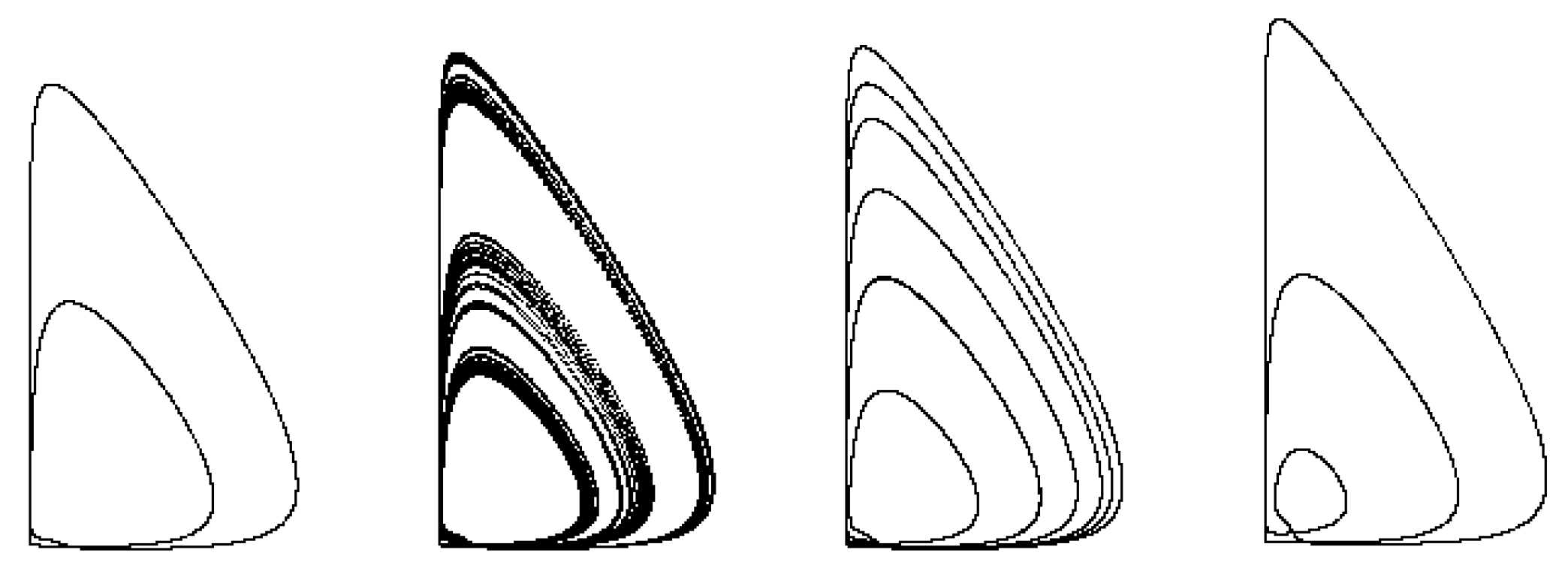
With a further decrease in the values of the parameter k, a sequence of stable cycles is found in accordance with the Sharkovsky order. So, for example, the cycle of period twelve of the subharmonic cascade exists at $k=10.093$, the cycle of period ten exists at $k=10.0897$, the cycle of period six exists at $k=10.086$, the cycle of period seven exists at $k=10.0658$, the cycle of period five exists at $k=10.057$ and, finally, the cycle of period three, which completes the subharmonic cascade of Sharkovsky bifurcations, exists at $k=10.03$ (Figure 2). Figure 2 also shows one of the singular subharmonic attractors of System (1) found for $k=10.07$.

As is known (see (1)–(3)), the last cycle of the subharmonic cascade of bifurcations, the cycle of period three, is the third cycle of the homoclinic cascade, the sequence of cycles of which must converge to the separatrix loop of the saddle-focus singular point $O$; however, for a given set of values of the system parameters, not only the separatrix loop does not exist in it but also the cycles of the homoclinic cascade, starting from the cycle $H_4$, which makes four successive revolutions around the singular point.

Thus, it has been numerically established that in System (1), as the values of the parameter k change, a cascade of Feigenbaum period-doubling bifurcations of stable limit cycles, a complete subharmonic cascade of bifurcations of stable cycles in accordance with the Sharkovsky order, and an incomplete homoclinic cascade of Magnitskii bifurcations are realized. Some cycles of the subharmonic cascade of bifurcations in the system of Equation (1) and one of the systems singular attractors in the sense of the FShM theory are shown in Figure 2.

3. Bifurcations and Chaos in the Model of a Chemical Process with Mutation

Let us consider the model of autocatalytic chemical reactions with mutation proposed in [25], in which the autocatalyst undergoes a mutation process in a fully stirred tank reactor. The model of autocatalytic reactions with mutation proposed in [25] is described by a system of nonlinear differential equations

$$\begin{array}{c}\dot{x}=-\frac{x}{\theta }+\left(1+\alpha \right){\gamma }_1\left(1-x\right)y^2+\beta {\gamma }_1\left(1-x\right)z^2\\ \dot{y}=\frac{\left(\delta -y\right)}{\theta }+\left(1-\alpha \right){\gamma }_1\left(1-x\right)y^2-{\gamma }_{2}y,\\ \dot{z}=-\frac{z}{\theta }+\beta {\gamma }_1\left(1-x\right)z^2+2\alpha {\gamma }_1\left(1-x\right)y^2-({\gamma }_2/\beta )z.\end{array}$$

(2)

System (2) has six parameters: $\alpha ,\beta ,\theta ,{\gamma }_1,{\gamma }_2,\delta .$ In [25], the last three parameters are fixed (${\gamma }_1=450,{\gamma }_2=11.25,\delta =0.067$), and several cases with different values of mutation coefficients α and its efficiency β are considered. In this case, the coefficient θ is a bifurcation parameter. Chaos in System (2) was discovered in [25] at $\alpha$ = 0.29,$\beta$ = 0.68 and with a change in the bifurcation parameter in the interval $0.10902\le \theta \le 0.10984$. For $\theta \approx 0.10902$ in System (2), a hard loss of stability of the singular point occurs. The cycle becomes stable, and as the values of the bifurcation parameter increase, it undergoes the Feigenbaum cascade of period-doubling bifurcations. A stable cycle of period two is born at $\theta \approx 0.10937,$ a cycle of period four is born at $\theta \approx 0.10642$, a cycle of period eight is born at $\theta \approx 0.10973$, etc. Then, at $\theta =0.10984$, chaotic dynamics was discovered in the system, which, according to the authors of [25], is confirmed by the found numerically positive value of the Lyapunov exponent, and the transition to chaos occurs allegedly through “intermittency”. The question of the nature of the chaotic dynamics found in System (2) by the authors of the paper [25] also remains open.

3.1. Subharmonic Chaos in the System of Equation (2)

System (2) has several singular points, two of which play the main role in the formation of chaotic dynamics since they have homoclinic and heteroclinic separatrix contours for the corresponding values of the system parameters. Equating the right parts of System (2) to zero, we find the coordinates of these two singular points $O_1$ and $O_2$

$$y_{\mathrm{1,2}}\left(x\right)=\frac{\left(1+{\gamma }_2\theta \right)\mp \sqrt{{\left(1{+\gamma }_2\theta \right)}^2-4\left(1-\alpha \right){\gamma }_1\left(1-x\right)\theta \delta }}{2\left(1-\alpha \right){\gamma }_1\left(1-x\right)\theta },$$

$$z_{\mathrm{1,2}}\left(x\right)=\sqrt{\frac{x}{{\theta \gamma }_1\beta \left(1-x\right)}-\frac{\left(1+\alpha \right)}{\beta }{y}_{\mathrm{1,2}}^2\left(x\right)},$$

and $x_{\mathrm{1,2}}$ are the solutions of the equation

$$\delta +x-\left(1+{\gamma }_2\theta \right)y_{\mathrm{1,2}}\left(x\right)-\left(1+\frac{{\gamma }_2\theta }{\beta }\right)z_{\mathrm{1,2}}\left(x\right)=0.$$

The Feigenbaum period-doubling bifurcation cascade in System (2), found in [25], occurs after a hard loss of stability of the singular point $O_1$ and continues along the parameter θ up to the value $\theta \approx 0.1098,$ at which the Feigenbaum singular attractor exists in the system. Feigenbaum attractor is the first non-periodic bounded trajectory, which is the limit of the cascade of period-doubling bifurcations of the original cycle. With a further increase in the values of the parameter θ, an incomplete subharmonic cascade of Sharkovsky bifurcations is realized in the system. A stable cycle of period six exists in System (2) at $\theta =0.10981$, and a cycle of period five exists at $\theta =0.10995.$ Further, the dynamics of solutions is simplified. Thus, a stable cycle of period six again exists in the system at $\theta =0.11016$, a cycle of period four exists at $\theta =0.11021$, and a cycle of period two exists at $\theta =0.1104.$ Consequently, the bifurcation scenario considered in [25], firstly, fits into the framework of the universal bifurcation FShM scenario. Secondly, the chaotic attractor that exists in System (2) at $\theta =0.10984$ is a trajectory lying in the neighborhood of a singular attractor formed by a cycle of period six from the subharmonic cascade of Sharkovsky bifurcations. Third, since for the considered values of the parameters, the complication of the dynamics of solutions of the system of Equation (2) does not even reach the birth of a stable cycle of period three, which completes the Sharkovsky cascade, the subharmonic attractor found in [25] is one of the simple chaotic attractors that exist in the System (2).

3.2. Homoclinic Chaos in the System of Equation (2)

Let us now show that System (2) has a much more complicated chaotic dynamics than the dynamics found in [25]. In order to find more complex singular attractors of System (2) in accordance with the Feigenbaum–Sharkovsky–Magnitskii theory, it is necessary to correctly determine which of the system parameters is bifurcational. We fix the last five parameters of the system ($\beta =0.68,\theta =0.10948,{\gamma }_1=450,{\gamma }_2=11.27,\delta =0.067$) and make the parameter α as a bifurcation parameter and consider the bifurcations occurring in System (2) as the values of the parameter α decrease in the interval $0.1876\le \alpha \le 0.3280$. For $\alpha \approx 0.328$ in System (2), a hard loss of stability of the singular point $O_1$ occurs. The cycle becomes stable, which, as the values of the bifurcation parameter decrease, undergoes a cascade of the Feigenbaum period-doubling bifurcations. A stable cycle of period two is born at $\alpha \approx 0.319$, a cycle of period four is born at $\alpha \approx 0.301$, a cycle of period eight is born at $\alpha \approx 0.297, \mathrm{e}\mathrm{t}\mathrm{c}.$ The Feigenbaum bifurcation cascade ends with a singular Feigenbaum attractor that exists in System (2) at $\alpha \approx 0.296$. As the values of the bifurcation parameter α decrease further, a complete subharmonic cascade of Sharkovsky bifurcations is realized in System (2). So, for example, a cycle of period five exists in the system at $\alpha =0.292$, and a cycle of period three, which completes the Sharkovsky cascade, exists in System (2) in the interval $0.279\le \alpha \le 0.2867$ (see Figure 3).

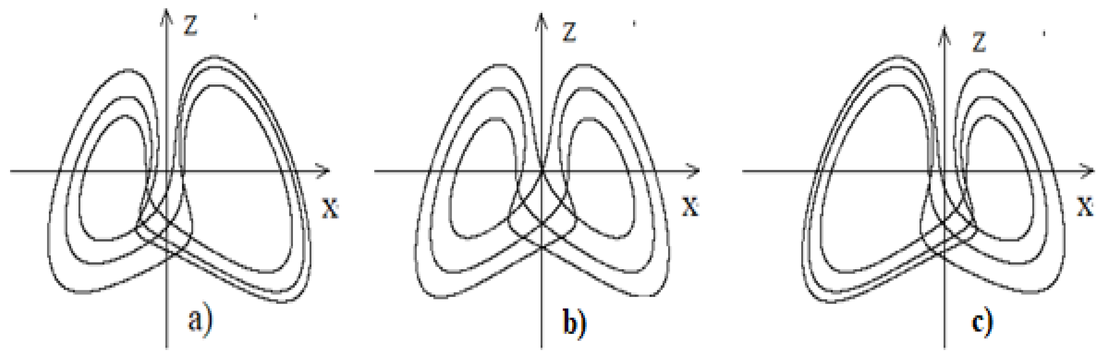
With a further decrease in the values of the parameter $\alpha$ in System (2), an incomplete homoclinic cascade of Magnitskii bifurcations of the birth of stable homoclinic cycles is realized, converging to a homoclinic contour, which is the saddle-focus separatrix loop of the singular point $O_1$. The homoclinic cascade begins with a cascade of bifurcations of period-doubling of the cycle of period three of the Sharkovsky cascade, which is also a homoclinic cycle of period three. A stable homoclinic cycle of period four exists in System (2) at $\alpha =0.2592,$ a homoclinic cycle of period five exists at $\alpha =0.2417,$ and a homoclinic cycle of period six exists at $\alpha =0.237$ (Figure 4).

With a further decrease in the values of the parameter α, the dynamics in System (2) is simplified in the reverse order of the FShM cascade of bifurcations, ending with a stable simple cycle gently sticking into the unstable singular point $O_1$ at $\alpha \approx 0.1876.$ Thus, for the given values of the parameters in System (2), there is no homoclinic loop of the separatrix of the singular point of the saddle-focus type, and the homoclinic chaos that exists in the neighborhood of homoclinic cycles is rather complicated but not the most complicated chaos that can, in principle, exist in System (2). The problem of finding in the space of parameters the hypersurface of the existence of homoclinic loop of a saddle-focus separatrix is an independent and rather complicated problem and is not considered in this paper.

3.3. Heteroclinic Chaos in the System of Equation (2)

In System (2), for some values of the parameters, there apparently exists a heteroclinic separatrix contour connecting the singular points $O_1$ and $O_2$ and, possibly, a homoclinic contour (separatrix loop) of the singular point $O_2$. One of the stable heteroclinic cycles that exists in the neighborhood of the separatrix heteroclinic contour of the singular points $O_1$ and $O_2$, and found for the values of the parameters $\theta =0.11,\alpha =0.2538$, is shown in Figure 5. Figure 5 also shows heteroclinic chaos in System (2) at $\theta =0.11,\alpha =0.254,$ generated by the singular attractor of the system in the neighborhood of its heteroclinic cycle. From Figure 5, it can be seen that somewhere in the neighborhood of the heteroclinic cycle, there must also be a homoclinic separatrix contour of the singular point $O_2$.

4. Bifurcations and Chaos in a Model of the Numbers of Interacting Populations

In [26], A.D. Bazykin et al. proposed a model for the dynamics of the interacting populations of a predator and two preys. The model is a system of three nonlinear ordinary differential equations

$$\begin{array}{c}\dot{x}=x\left(\alpha -x-\beta y-4z\right),\\ \dot{y}=y\left(\delta -y-x-10z\right),\\ \dot{z}=z\left(-1-x/4+4y-z\right)\end{array}$$

(3)

with positive fixed parameters $\alpha$ = 11, $\beta$ = 6 and a changing bifurcation parameter δ, which is the growth rate of the second prey. It was numerically shown in [26] that as the values of the parameter δ decrease in System (3), a cascade of period-doubling bifurcations of stable limit cycles is observed. In [27], a hypothesis was put forward that such a cascade is a transition to a complex inexplicable quasi-stochastic dynamics. The purpose of this work is to show that the dynamics of the numbers of interacting populations in Model (3) is completely subject to the universal law of transition to dynamical chaos in nonlinear systems of differential equations in accordance with the bifurcation scenario of Feigenbaum–Sharkovsky–Magnitskii.

4.1. Dissipativity Region and Singular Points of the System (3)

System (3) has seven singular points:

(1) $x_{*}=y_{*}=z_{*}=0;$ (2) $x_{*}={\alpha ,y}_{*}=z_{*}=0$; (3) $x_{*}=0,y_{*}=\delta ,z_{*}=0;$ (4) $x_{*}=y_{*}={0,z}_{*}=-1$; (5) $x_{*}=0,y_{*}=(10+\delta )/41,z_{*}=(-1+4\delta )/4(1;$ (6) $z_{*}=0,x_{*}=(11-\beta \delta )/(1-\beta ),y_{*}=(\delta -11)/(1-\beta );$ (7) $y_{*}=(\alpha +4)/(\beta +16),x_{*}=-(\delta +10)/1.5+27.33333y_{*},z_{*}=-1-x_{*}/4+4y_{*}.$

We are interested in the dynamics of solutions to System (3) in the neighborhood of the seventh singular point $O$ with nonzero coordinates ${(x}_{*},y_{*},z_{*}),$ the neighborhood in which complex irregular dynamics can exist. Let $\alpha =10, \beta =3.4$ and study System (3) for $10.9<\delta <13.1$. Let us calculate the divergence of the vector field of the system

$$div \mathit{F}\left(x_{*},y_{*},z_{*}\right)=\left(\frac{\partial F_1}{\partial x}+\frac{\partial F_2}{\partial y}+\frac{\partial F_3}{\partial z}\right)\left(x_{*},y_{*},z_{*}\right)=-\left(x_{*}+y_{*}+z_{*}\right)<0$$

everywhere in the region under consideration, where $F_i,i=\mathrm{1,2},3$ are the right parts of the equations of the system. Consequently, System (3) is dissipative in a neighborhood of the singular point $O{(x}_{*},y_{*},z_{*})$ for all considered values of the parameter δ.

4.2. Stability Region and Andronov–Hopf Bifurcation of a Singular Point of System (3)

Let us study the stability of the singular point $O{(x}_{*},y_{*},z_{*})$ of System (3). The linearization matrix of the right side of the system at a singular point has the form:

$$A=\left(\begin{array}{ccc}-x^{*},& -3.4x^{*},& -4x^{*}\\ -y^{*},& -y^{*},& -10y^{*}\\ -0.25z^{*}& 4z^{*}& {-z}^{*}\end{array}\right)$$

and its characteristic equation is the equation:

$${\lambda }^3+\left(x_{*}+y_{*}+z_{*}\right){\lambda }^2+\left({41z}_{*}-2.4x_{*}\right)y_{*}\lambda +29.1x_{*}{y}_{*}{z}_{*}=0.$$

Theorem 2.

The singular point $O$ of System (3) is asymptotically stable for $\delta >{\delta }_{*}\approx 13.0939.$ For $\delta <{\delta }_{*}$, the singular point $O$ becomes unstable, and, as a result of the Andronov–Hopf bifurcation, a stable limit cycle is softly born from it.

Proof. 

Let us rewrite the characteristic equation in the form

$${\lambda }^3+a_1\left(\delta \right){\lambda }^2+a_2\left(\delta \right)\lambda +a_3\left(\delta \right)=0.$$

By virtue of the Routh–Hurwitz criterion, a singular point $O$ is asymptotically stable if and only if

$$a_1\left(\delta \right)>0,a_2\left(\delta \right)>0,a_3\left(\delta \right)>0,a_1\left(\delta \right)a_2\left(\delta \right)>a_3\left(\delta \right).$$

Since $a_1\left(\delta \right)>0$ for $\delta <26.644$, $a_2\left(\delta \right)>0$ for $\delta >11.1933,$ $a_3\left(\delta \right)>0$ for $8.881<\delta <21.067$, and $a_1\left(\delta \right)a_2\left(\delta \right)>a_3\left(\delta \right)$ for $13.0939<\delta <50.6845,$ then the singular point $O$ of System (3) is asymptotically stable for $13.0939<\delta <21.067$. For $\delta <{\delta }_{*}\approx 13.0939$, the singular point $O$ becomes unstable, and in this case $a_1\left(\delta \right)a_2\left(\delta \right)<a_3\left(\delta \right).$ At the bifurcation point $\delta ={\delta }_{*}$, we have $a_1\left(\delta \right)a_2\left(\delta \right)=a_3\left(\delta \right).$ Let us show that for such a value of ${\delta }_{*}$ in System (3), the limit cycle is softly born from the singular point $O$ as a result of the Andronov–Hopf bifurcation. Indeed, if at the point ${\delta }_{*}$ the Routh–Hurwitz conditions for the coefficients of the characteristic equation and the condition $a_1\left(\delta \right)a_2\left(\delta \right)=a_3\left(\delta \right)$ are satisfied, the characteristic equation can be rewritten as

$$({\lambda }^2+a_2\left({\delta }_{*})\right){(\lambda +a}_1\left({\delta }_{*}\right))=0.$$

Therefore, at the point ${\delta }_{*}$, the roots of the characteristic equation have the form: ${{\lambda }_1=-a}_1\left({\delta }_{*}\right)<0,$ ${\lambda }_2=i\sqrt{a_2\left({\delta }_{*}\right)},$ ${\lambda }_3=-i\sqrt{a_2\left({\delta }_{*}\right)}$, that is, the characteristic equation has one real negative root and two complex conjugate roots, which is the condition for the Andronov–Hopf bifurcation at the point ${\delta }_{*}.$ The theorem is proved. □

From Theorem 2, it follows that the greatest interest is the study of possible cascades of bifurcations for $\delta <{\delta }_{*}$ of a stable limit cycle born from a singular point $O$ at $\delta ={\delta }_{*}$ as a result of the Andronov–Hopf bifurcation. It is in this case that all three cascades of bifurcations of stable limit cycles and an infinite number of chaotic singular attractors can exist in System (3) in accordance with the universal Feigenbaum–Sharkovsky–Magnitskii bifurcation theory.

The study of the following bifurcations with decreasing values of the bifurcation parameter $\delta <{\delta }_{*}$ by analytical methods starting from the bifurcation of doubling the period of the born limit cycle is an extremely difficult task; therefore, further study of the complication of the dynamics of solutions of the system of Equation (3) will be carried out by numerical methods

4.3. Scenario of Transition to Chaos in System of Equation (3)

Let us carry out a numerical study of System (3) with fixed values of the parameters α = 10.7, β = 3.4 and a decrease in the values of the bifurcation parameter $\delta <{\delta }_{*}=13.0939$. At $11.1<\delta <{\delta }_{*}$, in System (3) the Feigenbaum cascade of period-doubling bifurcations of stable cycles is observed. So, at $\delta =11.18$ in System (3), there is a stable (asymptotically orbitally stable) limit cycle of the double period, at $\delta =11.13$ there is a stable cycle of period four, at $\delta =11.11$ there is a stable cycle of period eight, etc. For smaller values of the parameter $\delta$, System (3) reveals a sequence of stable cycles of a subharmonic cascade of bifurcations in accordance with the Sharkovsky order. So, for example, the cycle of period six of the subharmonic cascade exists at $\delta =11.09,$ and the cycle of period three, which completes the Sharkovsky cascade, exists at $\delta =11.031$ (Figure 6).

As is known (see (1)–(3)), the last cycle of the subharmonic cascade of bifurcations—the cycle of period three—is the third cycle of the homoclinic cascade, the sequence of cycles of which must converge to the separatrix loop of the saddle-focus singular point $O$. Figure 7 shows the stable cycles of the homoclinic cascade of periods four and five, as well as one of the singular homoclinic attractors of System (3) for $\delta =10.97,$ which lies in the neighborhood of the separatrix loop of the saddle-focus singular point $O$.

Thus, it has been numerically established that in System (3), as the values of the parameter δ change, a Feigenbaum cascade of period-doubling bifurcations of stable limit cycles is realized, as well as complete subharmonic cascade of bifurcations of stable cycles in accordance with the Sharkovsky order and an incomplete homoclinic cascade of Magnitskii bifurcations. Some cycles of subharmonic and homoclinic cascades of bifurcations and singular attractors in the sense of the FShM theory are shown in Figure 6 and Figure 7.

5. Traveling Waves and Space-Time Chaos in the Model of the Numbers of Interacting Populations

Consider a spatio-temporal model of the dynamics of numbers of interacting populations, which is a system of equations in partial derivatives of the reaction–diffusion type

$$\left\{\begin{array}{c}{u}_t=D_1{u}_{xx}+\left(\mu +1\right)u^2-u^{3}v-A\\ v_t=D_2{v}_{xx}+u^{3}v-\mu u^2\end{array}\right.$$

(4)

By linearization in the neighborhood of the thermodynamic branch $\left(U,V\right)=(\sqrt{A},\mu /\sqrt{A}$), System (4) can be reduced in the first approximation to the system

$$\left\{\begin{array}{c}{z}_t=D_1{z}_{xx}+\sqrt{A}\left(2-\mu \right)z-\sqrt{A^3}y\\ y_t=D_2{y}_{xx}+\sqrt{A}\mu z+\sqrt{A^3}y,\end{array}\right.$$

where $u=\sqrt{A}+z,v=\mu /\sqrt{A}+y$. Therefore, for $0<\mu <2$, the dynamics of system of Equation (4) in the neighborhood of its thermodynamic branch is the dynamics of the interaction between the numbers of the predator described by the variable y, and the numbers of the prey described by the variable z.

Let us turn to the analysis of the dynamics of solutions and the transition to space-time chaos in the system of partial differential Equation (4). Let us prove that, for certain values of the parameters, System (4) has, in full accordance with the universal bifurcation theory of Feigenbaum–Sharkovsky–Magnitskii, an infinite number of different stable wave solutions travelling along the spatial axis with arbitrary velocities, as well as an infinite number of different regimes of space-time chaos. Moreover, the bifurcation parameter is the velocity of propagation of traveling waves along the spatial axis, which is clearly not included in the original system of equations.

5.1. Reduction to an ODE System by Means of a Self-Similar Change of Variables

Consider System (4) on the entire real axis: $u\left(x,t\right):\mathbb{R}\times \mathbb{R}\to \mathbb{R},v\left(x,t\right):\mathbb{R}\times \mathbb{R}\to \mathbb{R}$. We will analyze regular and chaotic solutions of System (4) using a self-similar change of independent variables $\xi =x-ct$, thereby reducing the original system of Equation (4) to a system of nonlinear ordinary differential equations

$$\left\{\begin{array}{c}\dot{u}=r,\\ \dot{r}=(-cr+A-\left(\mu +1\right)u^2+v{u}^3)/D_1,\\ \dot{v}=s,\\ \dot{s}=(-cs+\mu u^2-v{u}^3)/D_2,\end{array}\right.$$

(5)

where the derivative is taken with respect to $\xi$. If ($u\left(\xi \right),r\left(\xi \right),v\left(\xi \right),s\left(\xi \right))$ is a solution of the system of ordinary differential Equation (5), then $(u\left(x-ct\right),v\left(x-ct\right))$ will be a solution of the system of equations in partial derivatives (4). In this case, traveling waves of the system of Equation (4) are described by the limit cycles of System (5), traveling impulses of the system of Equation (4) are described by saddle-foci separatrix loops of System (5), and space-time chaos of the system of Equation (4) is described by singular attractors of System (5) in the sense of the universal bifurcation FShM theory.

5.2. Dissipativity Region and Singular Points of the System (5)

Let us study the area of dissipativity of the System (5):

$$div \mathit{F}\left(u,r,v,s\right)=\frac{\partial F_1}{\partial u}+\frac{\partial F_2}{\partial r}+\frac{\partial F_3}{\partial v}+\frac{\partial F_4}{\partial s}=-\frac{c}{D_1}-\frac{c}{D_2}.$$

Since $D_1>0,D_2>0,$ the system of Equation (5) is dissipative everywhere for $c>0$. Let us find the singular points $O\left(u_{*},r_{*},v_{*}{,s}_{*}\right)$ of System (5) by equating the right-hand sides of its equations to zero. We get that $r_{*}=s_{*}=0,u_{*}=\sqrt{A},v_{*}=\mu /\sqrt{A}$, i.e., $O\left(u_{*},r_{*},v_{*}{,s}_{*}\right)=O\left(\sqrt{A},0,\mu /\sqrt{A},0\right).$

Let us study the stability and type of the singular point $O$ of the System (5). The linearization matrix of the right side of the system at the singular point has the form

$$A=\left(\begin{array}{cccc}0& 1& 0& 0\\ \frac{\sqrt{A}(\mu -2)}{D_1}& -\frac{c}{D_1}& \frac{\sqrt{A^3}}{D_1}& 0\\ 0& 0& 0& 1\\ -\frac{\sqrt{A}\mu }{D_2}& 0& -\frac{\sqrt{A^3}}{D_2}& -\frac{c}{D_2}\end{array}\right),$$

and its characteristic equation is the equation

$$\det \left(A-\lambda I\right)={\lambda }^4+\left(\frac{c}{D_1}+\frac{c}{D_2}\right){\lambda }^3+\left(\frac{\sqrt{A^3}}{D_2}+\frac{c}{D_1}\frac{c}{D_2}-\frac{\sqrt{A}(\mu -2)}{D_1}\right){\lambda }^2+\frac{c\sqrt{A}\left(A-\mu +2\right)}{D_1{D}_2}\lambda +\frac{{2A}^2}{D_1{D}_2}=0.$$

In the case $D_1{=D}_2=D$, which we will consider below, the characteristic equation has the form

$${{\lambda }^4+\frac{2c}{D}\lambda }^3+\left(\frac{c^2}{D^2}+\frac{\sqrt{A}(A-\mu +2)}{D}\right){\lambda }^2+\frac{c\sqrt{A}}{D^2}\left(A-\mu +2\right)\lambda +\frac{{2A}^2}{D^2}=0.$$

(6)

Theorem 3.

The singular point $O$ of System (5) is asymptotically stable and is a stable focus for $c>c_{*}=\sqrt{D\left(8A^2-B^2\right)/2B}.$ For $c<c_{*}$, the singular point $O$ becomes a saddle-focus, and from it, as a result of the Andronov–Hopf bifurcation, a stable limit cycle is softly born.

Proof. 

By virtue of the Routh–Hurwitz criterion, a singular point $O$ is asymptotically stable if and only if

$$\frac{2c}{D}>0,\frac{2c}{D}\left(\frac{c^2}{D^2}+\frac{B}{D}\right)-\frac{cB}{D^2}=\frac{c}{D}\left(\frac{{2c}^2}{D^2}+\frac{B}{D}\right)>0,\frac{cB}{D^2}\frac{c}{D}\left(\frac{{2c}^2}{D^2}+\frac{B}{D}\right)-{\left(\frac{2c}{D}\right)}^2\frac{{2A}^2}{D^2}>0,$$

where $B=\sqrt{A}\left(A-\mu +2\right)>0.$ The first inequality holds for all $c>0.$ The second inequality is also satisfied. Consequently, the singular point $O$ of System (5) is asymptotically stable for

$$\frac{{2c}^{2}B}{D}+B^2-8A^2>0,c>c_{*}=\sqrt{D\left(8A^2-B^2\right)/2B}.$$

Let us show that for $c<c_{*}$, a stable limit cycle is born from the singular point $O$, which corresponds to the transition of two complex conjugate roots of the characteristic Equation (6) from left to right through the imaginary axis of the plane of the complex variable. Indeed, let the value of the variable $c$ be such that the characteristic Equation (6) has the following roots: ${\lambda }_1<0,{\lambda }_2<0,{\lambda }_3=i\omega ,{\lambda }_4=-i\omega .$ Then, using the Vieta theorem, we have the equalities

$${{\lambda }_1+{\lambda }_2=-\frac{2c}{D},{\lambda }_1{\lambda }_2+{\omega }^2=\frac{c^2}{D^2}+\frac{B}{D},(\lambda }_1+{{\lambda }_2)\omega }^2=-\frac{cB}{D^2},{\lambda }_1{{\lambda }_2\omega }^2=\frac{{2A}^2}{D^2}.$$

By substituting from the first, third and fourth equalities the expressions for ${\lambda }_1+{\lambda }_2$, ${\omega }^2$ and ${\lambda }_1{\lambda }_2$ into the second equality, we get that it is satisfied for $c=c_{*}$. In this case, the transition through the imaginary axis of two complex conjugate roots of the characteristic equation occurs from left to right as the values of the variable $c$ decrease. That is, it is precisely for such a value of $c_{*}$ in the system of Equation (5) that the Andronov–Hopf bifurcation of the birth of a stable limit cycle occurs. The theorem is proved. □

It follows from Theorem 3 that the study of possible cascades of bifurcations of the singular point $O$ in the case when $c<c_{*}$ is of greatest interest. It is in this case that in System (5), the existence of all three cascades of bifurcations of stable limit cycles and an infinite number of chaotic singular attractors is possible in accordance with the universal Feigenbaum–Sharkovsky–Magnitskii bifurcation theory. Additionally, the system of Equation (4) can have an infinite family of the most complex periodic and non-periodic (chaotic) traveling waves up to traveling pulses. It also follows from Theorem 3 that the bifurcation parameter in the system of Equation (5) is the parameter $c$, which is not included explicitly in the original system of Equation (4) and characterizes the velocity of propagation of perturbations along the spatial axis x. Further study of the complication of the dynamics of solutions of the systems of Equations (4) and (5) will be carried out by numerical methods.

5.3. Scenario of Transition to Spatio-Temporal Chaos in System (4)

Numerical study of System (5) will be carried out at fixed values of the parameters $A=0.83,\mu =1.45$ and a decrease in the values of the bifurcation parameter $c<c_{*}\approx 3.954.$ A stable (asymptotically orbitally stable) limit cycle born at $c=c_{*}$ from a singular point $O$ of System (5) exists up to the value $c\approx 2.68$, at which point a stable limit cycle of doubled period is born from it. With a further decrease in the values of the parameter $c$ in System (5), the Feigenbaum cascade of cycle period-doubling bifurcations is observed. A Period four cycle is born at $c\approx 2.38$, a period eight cycle is born at $c\approx 2.315, \mathrm{e}\mathrm{t}\mathrm{c}.$ For $c\approx 2.29$, in System (5) there is the first simplest singular attractor—the Feigenbaum attractor—which is a non-periodic bounded trajectory, which is the limit of cycles from the Feigenbaum cascade.

With a further decrease in the values of the parameter $c$, a sequence of stable cycles is found in accordance with the Sharkovsky order. So, for example, the cycle of period six of the subharmonic cascade exists at $c=2.263,$ the cycle of period five exists at $c=2.17,$ and the cycle of period three, which completes the subharmonic cascade of bifurcations, exists at $c=2.01$ (Figure 8).

Thus, it has been numerically established that in System (5), as the values of the parameter c decrease, the Feigenbaum period-doubling cascade of stable limit cycles and the complete subharmonic cascade of bifurcations of stable cycles are realized in accordance with the Sharkovsky order. The found cycles of System (5) correspond to traveling waves of the system of Equation (4). Figure 9 shows such waves corresponding to the cycles and the singular attractor shown in Figure 8.

6. FShM Chaos in a System with a Hidden Attractor

In the modern literature on nonlinear and chaotic dynamics, the concept of a “hidden” attractor of an autonomous system of ordinary differential equations is widely used in the case when the system, together with an irregular attractor, either has no singular points at all (see [28,29]) or has stable singular points (see [30]). The system from [30] with a stable singular point was considered by the author in [3], where it was shown that its chaotic attractor is also a singular attractor generated by a subharmonic cascade of FShM bifurcations theory. The system of equations with “hidden” attractor and without singular points proposed in [28] has the following form

$$\dot{x}=a\left(y-x\right)-w,\dot{y}=xz,\dot{z}=b-xy,\dot{w}=x.$$

(7)

The “hidden” attractor was found by the authors of [28] in System (7) at $a=4,b=40$, and the allegedly positive Lyapunov exponent was calculated in MATLAB by integrating the equations of System (7) by the fourth-order Runge–Kutta method, that, as noted above, is an absolutely meaningless procedure and is not a characteristic of the attractor.

The fact that System (7) must have some attractor for all $a>0$ follows from its dissipativity since for the divergence of its right-hand side $\mathit{F}(x,y,z,w)$, we have

$$div \mathit{F}=\left(\frac{\partial F_1}{\partial x}+\frac{\partial F_2}{\partial y}+\frac{\partial F_3}{\partial z}+\frac{\partial F_4}{\partial w}\right)=-a<0.$$

Usually a complex singular attractor is born as a result of FShM cascade of stable cycle or torus bifurcations, which themselves are born as a result of one or two Andronov–Hopf bifurcations from an initially stable singular point. It is clear that this scenario does not work for System (7) since it has no singular points at all at $b\ne 0$, as in this case its right-hand sides cannot be equal to zero at the same time. Nevertheless, let us show numerically that the “hidden” attractor found in System (7) is also a complex singular attractor of FShM cascades of bifurcations with respect to the parameter $a$ of some initially stable limit cycles of System (7) not born from singular points as a result of Andronov–Hopf bifurcations, but rather those born as a result of saddle-node bifurcations.

Numerical Analysis of the Transition to Chaos in System (7)

We will study the dynamics of solutions of the system of Equation (7) by numerical methods for $b=40$ and for decreasing values of the bifurcation parameter $a<15.5$. Numerical analysis shows that at $a=15.48$, System (7) has three stable limit cycles, which can be reached by integrating the equations of the system with different initial conditions. Figure 10 shows the projections of these cycles on the plane $\left(x,z\right).$ As the values of the parameter $a$ decrease, the central symmetric cycle undergoes a fork-type bifurcation, remaining unstable in the system, and cascades of bifurcations occur with the two stable limit cycles born in this case, in full accordance with the theory FShM. So, stable cycles of period two are observed at $a=13.5,$ stable cycles of period four are observed at $a=13.37,$ stable cycles of period eight are observed at $a=13.36,$ and the first Feigenbaum singular attractors are observed at $a=13.34.$ Cycles of period three, completing the subharmonic cascades of Sharkovsky bifurcations, can be observed at $a=12.71$ (Figure 11a,c).

Further complication of the dynamics of solutions of the system of Equation (7) occurs, as in the system of Lorentz equations, by merging two tapes of heteroclinic separatrix manifolds containing all unstable cycles, with the appearance of a cascade of bifurcations of heteroclinic cycles. One of the stable heteroclinic cycles found at $a=10.3$ shown in Figure 11b.

With a further decrease in the values of the parameter $a$, new stable cycles are born as a result of saddle-node bifurcations found at $a=10.1$ and shown in Figure 12. With the cycles shown in Figure 12a,d, period-doubling bifurcations occur at $a=9.95$ and then complete subharmonic cascades of Sharkovsky bifurcations take place. The cycles shown in Figure 12b,c remain stable up to $a=9.25,$ and then also undergo full subharmonic cascades of Sharkovsky bifurcations.

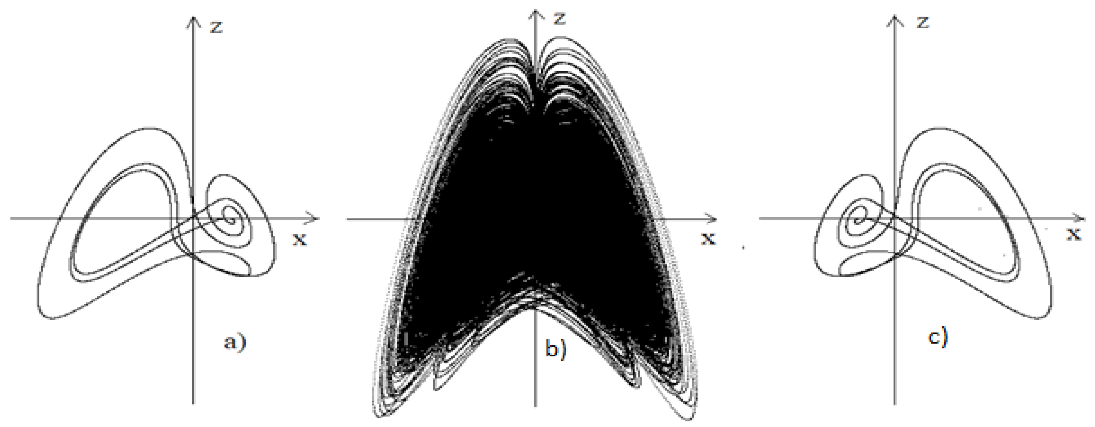
In Figure 13a,c the stable cycles of three periods found at $a=8.767$ are shown, which complete the subharmonic cascades of Sharkovsky bifurcations, the beginning of which is laid by the cycles shown in Figure 12b,c. In Figure 13b, the “hidden” attractor of the system of Equation (7) found by the authors of [28] for $a=4$ also is shown. The form of the “hidden” attractor clearly indicates its formation as a result of cascades of bifurcations of cycles, shown in Figure 10, Figure 11 and Figure 12. Thus, the so-called “hidden” attractor found in System (7) with $a=4$ is a consequence of several infinite cascades of bifurcations in accordance with the universal Feigenbaum–Sharkovsky–Magnitskii bifurcation scenario with decreasing values of the bifurcation parameter a. That is, the “hidden” attractor of System (7) is not some special type of irregular attractors, but just like in any other three-dimensional and multidimensional nonlinear dissipative and conservative systems of ordinary and partial differential equations, it is one of an infinite number of singular attractors of the system. Since all cycles that are born and become unstable at all stages of all FShM cascades of bifurcations do not disappear, but rather remain in the system, the complexity of the singular attractors of System (7) increases significantly with the decreasing values of the parameter a, and the stability regions of the resulting saddle-node bifurcations of new stable cycles are significantly reduced, which significantly limits the possibility of finding them numerically for $a\gtrsim 4$, although undoubtedly, such stable cycles must also exist in the interval $4<a<8.7$.

Thus, a numerical study of the nature of “hidden” attractors of nonlinear autonomous systems of differential equations has been carried out using the example of an irregular attractor of System (7). It is shown that the transition to the attractor in this nonlinear system of differential equations occurs, as in any other nonlinear chaotic systems of differential equations, in accordance with the universal Feigenbaum–Sharkovsky–Magnitskii bifurcation scenario. At the same time, due to the absence of singular points and, consequently, the absence of homoclinic and heteroclinic separatrix contours, several incomplete FShM cascades of bifurcations are realized in the system, forming an infinitely sheeted surface of a two-dimensional heteroclinic separatrix manifold (separatrix zigzag) containing both all singular attractors of the system and all its unstable limit cycles. The leading characteristic Lyapunov exponent on any singular attractor of the system is zero, and its positive values found numerically are only the result of computational errors

7. Conclusions

In this work, an analytical and numerical analysis of laminar–turbulent transitions in five nonlinear systems of ordinary and partial differential equations, which are models of autocatalytic chemical processes, the numbers of interacting populations and “hidden” attractor is carried out. It is numerically shown that in all considered systems of equations, the transition to chemical and biological turbulence is carried out in full accordance with the universal Feigenbaum–Sharkovsky–Magnitskii bifurcation theory through subharmonic and homoclinic cascades of bifurcations of stable limit cycles. It is proved that irregular attractors in all cases are exclusively singular attractors in the sense of the FShM theory.

Let us make some general remarks about the causes and scenarios of the emergence of chaos in nonlinear systems of differential equations. The discussion in [25,28,29,30] and many others published papers about “hyperchaotic”, “hidden”, “strange”, “stochastic”, “hyperbolic” and other attractors even in prestigious refereed journals, indicates to a complete lack of understanding how chaotic dynamics in nonlinear systems of differential equations appears. In this paper, the author’s papers [1,2,3] and many other papers have convincingly demonstrated with numerous examples that there exists a universal FShM bifurcation scenario of transition to dynamical chaos in all nonlinear systems of ordinary, partial and delay differential equations: autonomous and non-autonomous, dissipative and conservative. Only singular attractors can appear during the realization of this scenario, and infinitely many structurally different singular attractors can exist in nonlinear system for different values of the bifurcation parameter. This bifurcation parameter may not be included explicitly into the equations of the system. Thus, the presence or absence of homoclinic or heteroclinic separatrix contours in the system, presence or absence of stable or unstable singular points are not a condition for the appearance of dynamical chaos in the system. The existence of positive numerically defined senior Lyapunov exponent or Smale’s horseshoe and the consequences of KAM theory and the theory of RT also are not such conditions. The effect of calculating of the positive Lyapunov exponent is exclusively a consequence of numerical errors. Numerical trajectory of the singular attractor must move not along its real trajectory but only over the entire region in which it is located since this region filled of everywhere dense set of periodic and non-periodic unstable orbits. In addition, the calculated Lyapunov exponent can be also positive if it is the exponent of a stable periodic orbit of a large period located in the neighborhood of singular attractor. Smale’s horseshoe indicates to the complex dynamics in the system; however, even presence of infinite number of Smale’s horseshoes in the neighborhood of the saddle-focus separatrix loop does not confirm the chaotic dynamics. It can be confirmed only by a much more complex set of unstable periodic and non-periodic solutions born at all stages of all bifurcation cascades of the FShM scenario, which ends with a saddle-focus separatrix loop. The presence of chaos in the system of nonlinear differential equations can be confirmed only by the numerical finding of some main stable cycles or tori of the FShM cascades of bifurcations in accordance with the universal bifurcation diagram.