Reversible Data Hiding in Encrypted Image Based on Bit-Plane Redundancy of Prediction Error

Abstract

In this paper, we propose a reversible data hiding scheme in an encrypted image based on bit-plane redundancy of prediction error. The scheme greatly improves the embedding capacity while maintaining lossless image recovery and error-free secret data extraction. Firstly, the original image is preprocessed to obtain the prediction error image. After the error matrix is divided into blocks, the corresponding block type is obtained. Secondly, the predicted error image is encrypted with stream cipher and the encryption matrix blocks are scrambled to ensure the security of the scheme. Finally, after embedding the block type value into the encrypted image, the spare room corresponding to each block was obtained, which was used to embed the secret data. The scheme makes full use of the spatial correlation of the pixels in the block, so it improves the embedding rate. By selecting 100 images in each dataset of BOSSbase and BOWS-2, when the block size is $3\times 3$, the average embedding rate of our scheme can reach 3.56 bpp and 3.81 bpp, respectively. The performance of the proposed method is better than the other schemes with similar properties.

1. Introduction

Reversible data hiding is a technology which hides secret data in an information carrier, which can recover the original carrier without distortion and extract secret data without error. The information carrier can be sound, image, video and so on. In general, reversible data hiding is used in certain scenarios where the carrier requires lossless recovery, such as in military images, medical image diagnosis, and judicial forensics. In recent years, a large number of scholars have proposed many reversible data hiding schemes [1,2,3,4,5,6,7,8,9,10,11,12,13,14,15,16,17,18,19,20,21,22]. Reversible data hiding is mainly divided into the following four categories: lossless compression-based schemes [1,2], which generate spare room for hiding data through the lossless compression method, and recovers the original carrier and secret data after decompression to achieve the effect of lossless hiding. Difference expansion (DE)-based schemes [3,4,5], which propose to take two pixels as a group, expand the difference of the pixels to embed secret data, and use the difference and the average value to obtain the new pixel with embedded data. Histogram shifting (HS)-based schemes [6], which use the peak point and zero point of the original image histogram and the pixels between the two points are shifted to hide the secret data. Prediction error expansion (PEE)-based schemes [7,8], which use the correlation between pixels to predict the pixel value and obtain the pixel error, where the error value is extended to embed the secret data.

With the development of cloud services and the enhancement of people’s awareness of privacy protection, reversible data hiding has gradually become combined with encryption technology to form reversible data hiding in encrypted image (RDHEI). It can not only ensure the security of the cover image, but also embed data without knowing the original content, without destroying the structure of the original carrier, so as to achieve privacy protection. The RDHEI scheme realizes double protection for the cover image and secret information. If it focuses on protecting secret information, the application scenario of the scheme is steganography. If it focuses on protecting images with authentication, the application scenario is watermarking.

According to whether the cover image needs to be preprocessed before encryption to create spare room for secret data embedding, the RDHEI is divided into two categories: reserving room before encryption (RRBE) and vacating room after encryption (VRAE). For RRBE-based frameworks, the spatial correlation of pixels is preserved before encryption to obtain higher embedding capacity. General compression methods, such as ZIP, can be used to implement RRBE-based reversible data hiding in encrypted image scheme, but it does not take into account the characteristics of the image, so the embedding capacity is limited. Therefore, many scholars try to compress the image by mining the characteristics of the cover image to obtain more available space to increase the overall embedding rate of the scheme. Ma et al. [9] embedded part of the least significant bit (LSB) of the pixels in the complex region into the smooth region, so as to reserve part of the LSB space of the pixels for embedding data. After that, the data extraction and image reconstruction of the scheme have no errors. Zhang et al. [10] improved the scheme [9] by shifting the histogram of certain pixel prediction errors to release room for data embedding before encrypting the image. The embedding rate and the peak signal-to-noise ratio (PSNR) of the decrypted image are improved. Wu et al. [11] proposed a reversible data hiding scheme in a Paillier cryptosystem, which preprocessed the plaintext image before encryption. The embedded data can be extracted directly in the ciphertext domain using homomorphism. The scheme achieves high data hiding ability, and can safely protect user privacy and data integrity. Yin et al. [12] adaptively predicted the multiple most significant bit (MSB) of each pixel and marked it by Huffman coding in the original image, and the image is encrypted by stream cipher. With multiple MSB replacement, the vacated space can be used to embed additional data. The method achieves high embedding capacity. Wu et al. [13] proposed to preserve the embedding space in the plaintext image before encryption and to label the encrypted pixels into two different categories using a parametric binary tree. The secret data is embedded in one of the two categories of encrypted pixels by bit replacement, and a higher embedding rate is achieved.

In VRAE methods, content owners do not need to preprocess images before encryption. Zhang et al. [14] proposed to embed additional data into the image by flipping 3LSBs of a small part of the encrypted data after encrypting the image with stream cipher. The receiver can obtain different available information through different permissions, but this scheme cannot achieve perfect data extraction and image recovery. Puteaux et al. [15] replaced the most significant bit of each available pixel in the encrypted image with a small portion of the secret data after encrypting the original image. The MSB prediction can extract the embedded data without error. The clear cover image is reconstructed without loss. Qin et al. [16] used stream cipher and block permutation to encrypt the original image block, and compressed the LSB of the block set in the smooth area of the encrypted image to create extra embedding space. According to the availability of the key, the receiver performs data extraction and image recovery, respectively.

In general, the embedding rate of VRAE-based scheme is relatively low because the encryption destroys the spatial correlation of the neighboring pixels of the image. In order to solve the above problems, many schemes use image block-based encryption methods, which can keep the correlation unchanged between pixels in each block before and after encryption. Chen et al. [17] divided the encrypted image into non-overlapping blocks and calculated the differences between reference pixels and other pixels within the blocks. By compressing the pixel difference to vacate room for hiding secret data. Wang and He [18] used uniform MSBs of pixels in the block to compress the block and obtained good results. However, this scheme wastes a lot of space in complex images. Fu et al. [19] determined embeddable blocks by analyzing the distribution of MSB layers in encrypted images, and then adaptively compressed the MSB layer of embeddable blocks to vacate space according to the occurrence frequency of MSBs. Pun et al. [20] used the traditional XOR method for block encryption to retain the redundancy in the encryption blocks. The redundant matrix existing in some encryption blocks generated available space to accommodate secret data, and the images directly decrypted by the scheme maintained high quality. Wang et al. [21] divided image blocks into available and unavailable blocks. Pixels in the available blocks share the same most significant bits, these blocks can be reconstructed to vacate room for data embedding. The hidden data can be extracted lossless, and the original image can be perfectly recovered. Gao et al. [22] divided the image into blocks, and used block permutation and block-level stream cipher to encrypt the image. The data hider analyzes the image blocks and adaptively determines the best block type label to encode them. The image is compressed to obtain empty rooms for embedding the encrypted secret data.

All the above methods do not make full use of the spatial correlation of pixels in the image blocks, so the payload is low. In this paper, a reversible data hiding scheme in encrypted images based on bit-plane redundancy of prediction error is proposed. On the premise of ensuring the security of the original image, the spatial correlation of the original image is extended to the prediction error image, and the correlation of the image pixels is fully utilized. The block type classification method was improved. The overall embedding capacity of the encrypted image was increased by implementing multi-level embedding on the error matrix. The receiver could extract the secret data without error and recover the original image lossless.

The rest of this paper is organized as follows. In Section 2, we review the related work. In Section 3, we briefly introduce the general framework and describe the details of the proposed scheme. In Section 4, we discuss the experimental results and the performance of the scheme. We conclude our method in Section 5.

2. Related Work

In this section, we introduce the tools used in this scheme, the Gradient-Adjusted Predictor and Huffman coding, as well as describe Gao et al.’s scheme in detail.

2.1. The Gradient-Adjusted Predictor [23]

The neighboring pixels of an image have high spatial correlation, and can be used to predict the target pixel value x. The Gradient-Adjusted Predictor (GAP) is the adaptive predictor, which adjusts according to seven different contexts around the predicted pixel. Its simplified version, namely SGAP, provides almost similar results to GAP, but is less computationally intensive. It uses four neighboring pixels of the target pixel x: left pixel($x_W$), upper left pixel($x_{NW}$), upper pixel($x_N$), upper right pixel($x_{NE}$), to predict its pixel value, as shown in Figure 1. The pixels of the first row, first column and last row as reference pixels remain unchanged during the prediction process.

2.2. Huffman Coding

Huffman coding is a lossless binary compression coding. It is not a fixed set of encoding, but according to the frequency of each character in the given information, the dynamic generation of the optimal encoding. The more characters appear, the shorter the encoding result. The fewer occurrences, the longer the encoding result. The purpose of Huffman encoding is to further compress the file; variable length encoding is used to compress the data to the shortest length.

2.3. Gao et al.’s Method [22]

(1) Block encryption: after dividing the original image into a series of non-overlapping blocks, block scrambling and block-level stream cipher encryption are carried out on the image blocks.

(2) Block-wise compression: the pixel in the lower right corner of the encryption block is taken as the reference pixel, and the whole image block is divided into nine types (0–8) according to the bit-plane characteristics of the pixel in the block and the reference pixel. The nine image block types are compressed and their values are marked with binary codes of the same length.

(3) Data embedding: the block type label is embedded into the highest bit-plane of the pixels in the block, and the secret data is embedded into the empty bit-plane.

(4) Image recovery and data extraction: the receiver extracts the corresponding block label set from the highest bit-plane of the pixels in the block after the image is divided into blocks. The secret information is extracted from the spare space. The remaining pixels in the block are recovered according to the partial bit-plane of the reference pixel, and the encryption key is used to decrypt and scramble the block to recover the original image.

3. Proposed Method

In this paper, a new high-capacity reversible data hiding in encrypted image based on bit-plane redundancy of prediction error is proposed, which can extract the secret data correctly and recover the original image losslessly. There are three users in this scheme, which are content owner, data hider and receiver. Figure 2 shows the framework of the proposed method.

The content owner first preprocesses the original image to obtain the prediction error image and the block type corresponding to the error matrix block. Then the prediction error image and matrix block are encrypted by stream cipher and scrambled, respectively. Finally, the block type was encoded and embedded into the block to obtain the final encrypted image and sent to the data hider.

The data hider extracts its corresponding block type value from the final encrypted image block and decodes it, calculates the spare space and embeds the encrypted secret data in it. The marked encrypted image is sent to the receiver.

The receiver divides the matrix in the marked encrypted image into blocks, extracts auxiliary information from image. According to different keys, the secret data can be extracted and the original image can be recovered, respectively.

3.1. Preprocessing

There are four stages in preprocessing: (1) using SGAP to obtain the prediction image corresponding to the original image, calculating the difference between the two images to obtain the prediction error image. (2) The error matrix in the prediction error image is divided into blocks to obtain the block types. (3) Block type merging. (4) Huffman code block type. The process is shown in Figure 3. In order to improve the embedding rate of the scheme, multi-level embedding can be performed on the reference error pixels.

3.1.1. Calculating Prediction Error

For the original image $I_o$ sized $M\times N$, the three-side edge pixels of the original image are denoted as $P_r$ and remain unchanged as reference pixels. The content owner uses the SGAP predictor to calculate the corresponding predicted pixel $px$ for x by Equation (1).

$$px=\frac{x_N+x_W}{2}+\frac{x_{NE}-x_{NW}}{4}$$

(1)

For pixel $x_{i,j}$, the predicted pixel generated according to Equation (1) is denoted as $p{x}_{i,j}$. All $p{x}_{i,j}$ and reference pixels $P_r$ form the predicted image $I_p$. Calculate the prediction error $e_{i,j}$ corresponding to each pixel of the original image $I_o$ and the predicted image $I_p$ except the reference pixel $P_r$ by Equation (2).

$$e_{i,j}=x_{i,j}-p{x}_{i,j},where2\le i\le M,2\le j\le N-1.$$

(2)

After the edge reference pixels are removed, all calculated prediction errors are formed an error matrix of size $(M-1)\times (N-2)$, denoted as P. This is shown in the yellow area of Figure 4.

A location map with the same size as matrix P is generated to record the positive and negative prediction errors, denoted as S-map. If the error value is negative, its corresponding position is 1, otherwise, its position is 0, which is used as auxiliary information $\xi 1$ for restoration of image pixels. As shown in Figure 5, an example of the process of generating a location map.

For the values in the error matrix P take their absolute value to obtain the matrix $P^{\prime }$. The prediction error image consisting of edge pixels $P_r$ and matrix $P^{\prime }$ is denoted as $I_{op}$.

3.1.2. Error Matrix Block Type

The content owner divides the error matrix $P^{\prime }$ of size $(M-1)\times (N-2)$ into n non-overlapping $s\times s$ sized blocks $B_i$ (i = 1, 2, $\dots$, n. $n=⌊\frac{(M-1)\times (N-2)}{s\times s}⌋$). Each small matrix block is processed in turn, every block contains $s^2$ prediction error values expressed by $e_t$, where t = 1, 2, $\dots$, $s^2$. Use the first error pixel $e_1$ in the block as the reference pixel. The prediction error values within the block are all converted into an 8-bit binary sequence using Equation (3).

$$e_t^k=⌊\frac{e_t}{2^{k-1}}⌋mod2,k=1,2,\dots ,8.$$

(3)

The prediction error pixels can be obtained by Equation (4).

$$e_t=\sum _{k=1}^8{e}_t^k\times 2^{k-1},k=1,2,\dots ,8.$$

(4)

For each matrix block B, the content owner in turn compares each bit of reference error pixel $e_1$ and the remaining $s^2$ − 1 prediction error pixels $e_t$ from MSB to LSB until a certain bit is different. Let $\alpha$ denote the length of the same bit for all error values in the block after comparison. The $\alpha$ bit of a pixel from the most significant bit is denoted as $\alpha MSB$. The former $\alpha MSB$ of all error pixels in each block are the same. There are nine different types of blocks at this point.

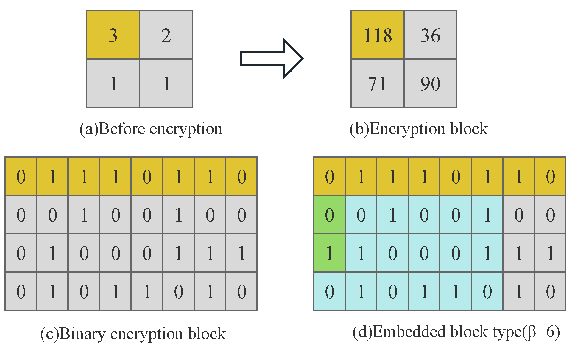
As shown in Figure 6, for a matrix block of size $2\times 2$, the reference error pixel is 3, and the remaining error pixels in the block are 2,1,1, respectively. Convert it all to an 8-bit binary sequence: ${\left(3\right)}_2=00000011,{\left(2\right)}_2=00000010,{\left(1\right)}_2=00000001$. After comparing its MSB to LSB in turn, it can be obtained that the six most significant bits are the same as (000000), and only two least significant bits are different. So, this matrix block corresponds to a block type value of 6.

3.1.3. Merge Block Types to Generate $\beta$-Map

After the content owner sequentially compares the MSB to the LSB of the error pixels in all predicted error blocks B, each matrix block has its corresponding block type $\alpha$ value, $\alpha \in$ 0, 1, 2, $\dots$, 8.

The number of blocks under nine different block types of smooth images Lena and Peppers, and complex images Baboon and Bridge were statistically analyzed in our experiment, as shown in

Table 1. Block distribution of different image in nine different block types ($\alpha$).

Image	0	1	2	3	4	5	6	7	8
Lena	0	12	965	4940	13,015	27,616	15,430	2393	654
Peppers	0	153	1429	5417	20,795	26,493	8887	1538	313
Baboon	1	3207	16,809	18221	16,826	8338	1411	184	28
Bridge	0	858	10,414	19727	18,380	11,322	3386	541	397

. Moreover, we experimented with more images and obtained similar results as in the table. The statistical results show that for smooth images with simple texture, the block types are mostly distributed in $\alpha$ = 4, 5, 6. The types of complex image blocks with rough texture were mostly distributed in $\alpha$ = 2, 3, 4. Therefore, we can merge the block type to reduce its unnecessary space in storage.

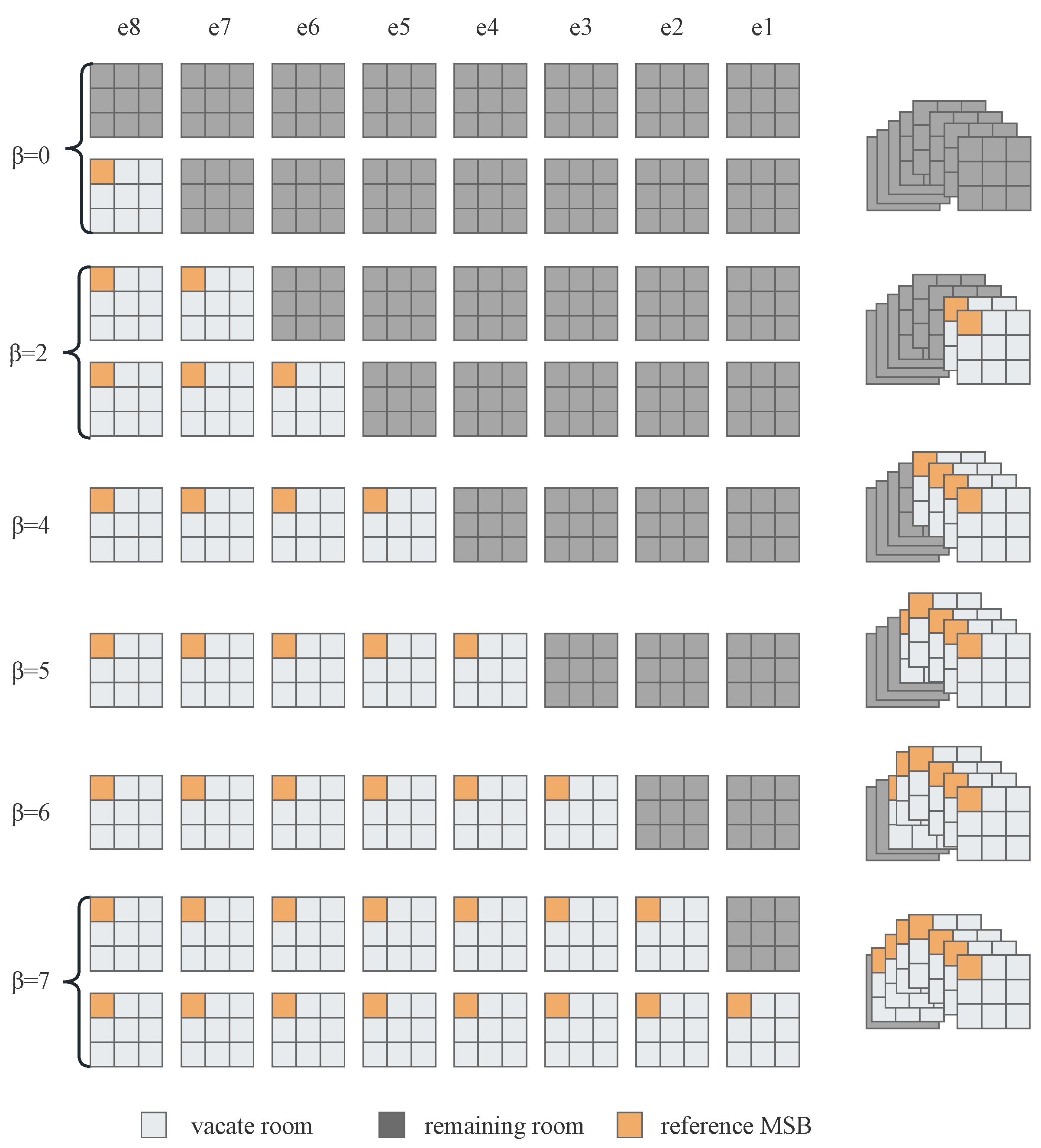
In this scheme, the block types are merged into six types. We use $\beta$ to denote the new block type value. For smooth images, if $\alpha$ = 0, 1, then $\beta$ = 0. If $\alpha$ = 2, 3, then $\beta$ = 2. For widely distributed block types, $\alpha$ = 4, 5, 6, then $\beta$ = 4, 5, 6 remains the same. If $\alpha$ = 7, 8, then $\beta$ = 7. The smoothed image yields six different block type labels, $\beta$ = 0, 2, 4, 5, 6, 7. For complex images, if $\alpha$ = 0, 1, then $\beta$ = 0. If $\alpha$ = 2, 3, 4, then $\beta$ = 2, 3, 4 remains unchanged. If $\alpha$ = 5, 6, then $\beta$ = 5. If $\alpha$ = 7, 8, then $\beta$ = 7. In this way, for complex images we obtain $\beta$ = 0, 2, 3, 4, 5, 7, six different block types. Each matrix block corresponds to a new fixed block type value, thus generating a label map $\beta$-map of size $⌊\frac{M-1}{s}⌋\times ⌊\frac{N-2}{s}⌋$.

Take a smooth image with simple texture with a block size of $3\times 3$ as an example, the spatial distribution of the bit-planes during the merging of the block type is shown in Figure 7. Where $e^1$–$e^8$ represents eight bit-planes.

For different $\beta$ values, the room that can be vacated by the corresponding block is $\beta (s^2-1)$. As shown in Figure 8, the original nine block types of the smoothed image are merged into six block types, where $B_c$ represents the space that can be vacated by different block types.

3.1.4. Huffman Encoding Compression $\beta$

Each matrix block corresponds to a fixed block type value, in this case for a smooth image ${\beta }_s$ = 0, 2, 4, 5, 6, 7. For complex images ${\beta }_c$ = 0, 2, 3, 4, 5, 7. $\beta \in \left\{{\beta }_s,{\beta }_c\right\}$. The n$\beta$ values obtained after processing the whole image prediction error matrix block. Six fixed-length Huffman codes $\left\{00,01,100,101,110,111\right\}$ were used to represent different six block types according to $\beta$ values.

The corresponding binary sequence after encoding is represented by $H\left(\beta \right)$. $L\left(\beta \right)$ is the length encoded by Huffman. $K\left(\beta \right)$ is the number of times different block types appear in the whole image. The coding rule is the auxiliary information $\xi 2$.

Table 2. Huffman coding sequence of Lena with block size of 2.

$\mathit{\beta }$	0	2	4	5	6	7
$K\left(\beta \right)$	12	5905	13,015	27,616	15,430	3047
$H\left(\beta \right)$	111	101	100	00	01	110
$L\left(\beta \right)$	3	3	3	2	2	3

takes the smooth image Lena with size 512 × 512 and block size 2 × 2 as an example, Huffman coding was used to obtain the coding value corresponding to each block type $\beta$.

Equation (5) is used to calculate the space capacity $SE{C}_i$ that can be vacated by each small block, where ${\beta }_i$ represents the corresponding block type value of block $B_i$.

$$SE{C}_i=(s^2-1)\times {\beta }_i-L\left({\beta }_i\right),where1\le i\le n.$$

(5)

The maximum embedding capacity of this algorithm is $MEC$, which is calculated as follows:

$$MEC={\sum }_{i=1}^{n}SE{C}_i$$

(6)

The block types are converted into binary sequences and concatenated with corresponding Huffman codes to generate 34 bits coding rules. Taking the smooth image Lena as an example, the coding rules are shown in Figure 9.

3.2. Image Encryption

After preprocessing, the content owner also needs to encrypt the image using the encryption key $K_e=\left\{K_{e1},K_{e2}\right\}$ to ensure the security of the scheme. The prediction error image $I_{op}$ composed of error matrix $P^{\prime }$ and unchanged image edge pixels $P_r$ was encrypted by stream cipher. Then, the prediction error matrix $P^{\prime }$ is divided into blocks and scrambled.

3.2.1. Stream Cipher Encrypts Image $I_{op}$

For the prediction error image $I_{op}$, the content owner uses the encryption key $K_{e1}$ to generate an $M\times N$ pseudo-random matrix R, and the matrix elements are denoted by $r_{i,j}$, $r\in [0,255]$. Using Equation (7), the pixels $Y_{i,j}$ corresponding to the image $I_{op}$ are encrypted by stream cipher.

$$E_{i,j}=r_{i,j}\oplus Y_{i,j},where1\le i\le M,1\le j\le N.$$

(7)

where ⊕ denotes the bitwise exclusive-or operation.

3.2.2. Block Scrambling

To further ensure the security of the encrypted image, the content owner scrambles the n error matrix blocks B using the encryption key $K_{e2}$. The key generates a sequence index of random natural numbers from 1 to n with no repetition $\left\{{\delta }_1,{\delta }_2,\dots ,{\delta }_n\right\}$. The matrix block B is scrambled with the index sequence to generate a new encryption block sequence $\left\{B_{{\delta }_1}^{\prime },B_{{\delta }_2}^{\prime },\dots ,B_{{\delta }_n}^{\prime }\right\}$.

After the above encryption process, the encrypted image $I_E$ is generated, the security of the image is guaranteed, and the spatial correlation of pixels in the block is not changed. If the selected s cannot completely divide the image into blocks, counts the row and column pixels that cannot be divided, and let its number be $\eta$. These pixels are encrypted using only stream cipher without subsequent block scrambling.

3.3. Data Hiding

3.3.1. Embedded Block Type $\beta$ Value

The content owner embedded the $\beta$-map into the encrypted image $I_E$. Firstly, the encryption error matrix $P_E^{\prime }$ in $I_E$ was divided into $s\times s$ blocks according to the same blocking method as in the preprocessing stage, the block scrambling key $K_{e2}$ was used to scramble the $\beta$-map to the corresponding matrix block position.

Then, all the reference error $e_t^{\prime }$ in the encryption block, $t=1,2,3,\dots ,s^2$ are converted to an 8-bit binary sequence using Equation (3), the first pixel $e_1^{\prime }$ in the encrypted small matrix block as a reference pixel remains unchanged during the embedding process. At last, the encoded values $H\left(\beta \right)$ for the corresponding block type $\beta$ are embedded into the partial MSB positions of the remaining $s^2-1$ error pixels $e_t^{\prime }$ in the block, where $t=2,3,\dots ,s^2$. The residual bit-plane remains the same.

For example, the original block in Figure 6 is encrypted by stream cipher to generate the encrypted block, the pixels in the encrypted block are converted into an 8-bit binary sequence, respectively. The encoded value $H\left(\beta \right)$ = 01 of the corresponding block type value $\beta$ = 6 for the original block is embedded into the MSB bit-plane of the error pixels $e_2^{\prime }$ and $e_3^{\prime }$ within the encrypted block, as shown in Figure 10.

In addition to that, the scheme needs to record the two or three bits of MSB replaced by the coded value within the matrix block with $\beta$ = 0 as auxiliary information $\xi 3$ to indicate that the block experiences overflow. Since the minimum of the block s = 2, the second to $L\left(\beta \right)$ + 1 bits of the most significant bit-plane of all pixels within each block represent the block type. The content owner sends the final encrypted image $I_E^{\prime }$ embedded with block type values to the data hider.

3.3.2. Secret Data Embedding

After receiving the final encrypted image $I_E^{\prime }$ sent by the content owner, the data hider first divides the error matrix $P_E^{\prime \prime }$ in the final encrypted image into small matrix blocks of size $s\times s$ and extracts the block type encoded values from the second to the fourth bit of the most significant bit-plane of all pixels in each block. The block type is recovered by decoding the encoded values using the encoding rules. Then, Equation (5) is used to calculate the space capacity $SE{C}_i$ that can be vacated for each small block. Finally, the embedded data is encrypted by stream cipher using the data hiding key $K_h$ to obtain the encrypted information $Mg$, which is embedded into the remaining former $\beta$MSBs for the $s^2-1$ pixels within the block except the reference pixel in turn.

For example, the blue area in Figure 10d can be used to embed secret data. The (8−$\beta$) LSBs of remaining $s^2-1$ pixels and the reference pixel remain unchanged before and after embedding the data.

3.3.3. Multi-Level Embedding

Generally, cover image pixels have high spatial correlation, which also exists for the prediction error pixels, so we can use this feature of pixels to obtain more redundant space. In the above preprocessing process, the reference error pixels in each block do not change. The content owner can extract all the reference error pixels in each matrix block to form a new error matrix, it is divided into blocks to find the corresponding block type label for each block, so as to create more extra room. The above operation can be repeated many times until the reference error matrix becomes a small matrix block that can no longer be segmented by the same method. The multi-level embedding process is shown in Figure 11.

The size of the final matrix block is denoted by $s^{\prime }$. This step can be repeated a different number of times for each different block size s, denoted as $\gamma$.

Table 3. Different blocks sizes correspond to embedding levels.

s	$\mathit{\gamma }$	${\mathit{s}}^{\prime }$
2	8	3
3	6	2
4	4	7
5	4	4
8	3	7

lists the final small matrix block sizes and the number of multi-level embeddings corresponding to different block sizes when the original image size is 512 × 512.

3.3.4. Auxiliary Information Embedding

Auxiliary information needs to be used in the data extraction and image restoration phases. Therefore, the receiver can successfully receive and extract with a specific method and embedding location. The auxiliary information of this scheme is given as follows.

(1)

The value of the block size, s, is represented by 4 bits.

(2)

It takes $(M-1)\times (N-2)$ bits to record S-map.

(3)

The Huffman coding rules for the six block types are represented by 34 bits.

(4)

A matrix block with overflow requires $K\left(\beta \right)\times L\left(\beta \right)$ bits, where $\beta$ = 0.

(5)

Multi-level embedding number $\gamma$ is represented by 3 bits.

(6)

The last embedded coordinate $(m,n)$ is represented by $lo{g}_2(m\times n)$ bits.

The three-side edge pixels $P_r$ of the original image are only encrypted with the stream cipher. We connect the auxiliary information to replace the LSB of these pixels. The length of the statistical auxiliary information is denoted as $L_{\xi }$, that is to replace $L_{\xi }$ LSBs of the reference pixel $P_r$. The length value $L_{\xi }$ and the replaced LSBs are connected in front of the secret data, and sequentially embed the information flow into the bit-planes vacated by each encryption block. The marked encrypted image $I_w$ is obtained. Send to the receiver.

The formula for calculating the payload of the scheme is as follows, where $ME{C}_i$ represents the maximum embedding capacity at each level of embedding.

$$EC={\sum }_{i=1}^{\gamma }ME{C}_i-L_{\xi }$$

(8)

3.4. Data Extraction and Image Recovery

In this scheme, data extraction and image recovery are separable. The content owner and the data hider send the encryption key and the data hiding key to the receiver through a specific information transmission channel. The receiver processes the marked encrypted image differently according to different permissions.

$\mathbf{Case}\mathbf{1}$: the receiver only has the data hiding key.

$\mathbf{Step}\mathbf{1}$: auxiliary information is extracted from the LSB of the edge pixels of the marked encrypted image $I_w$, including the value of the block size s, the S-map, the coding rules, the MSB of the overflow block replaced, the multi-level embedding level and the last embedding coordinate.

$\mathbf{Step}\mathbf{2}$: according to the block size s, the matrix $P_w^{\prime }$ in $I_w$ is divided into non-overlapping blocks $D_i$ of size $s\times s$.

$\mathbf{Step}\mathbf{3}$: the encoded value $H\left(\beta \right)$ is obtained by extracting the bit-plane consisting of $s^2$ pixels in $D_i$. The value of $\beta$ is decoded by Huffman coding rule, and the corresponding block location map $\beta$-map is recovered.

$\mathbf{Step}\mathbf{4}$: extract the first pixel in the block forms a new matrix. The above extraction steps 2 and 3 are repeated $\gamma$ times.

$\mathbf{Step}\mathbf{5}$: after knowing the type value of each block, extract the $L\left(\beta \right)+1$ bit to the $(s^2-1)\times \beta$ bit of the bit-plane of the remaining ($s^2-1$) pixels in each block except the reference pixel. Up to the last embedding coordinate of the corresponding levels.

$\mathbf{Step}\mathbf{6}$: the embedded information flow can be obtained by linking the extracted data together, from which the replaced LSB and the encrypted secret data $Mg$ are decomposed, and the data can be obtained after decrypting the $Mg$ with the data hiding key $K_h$.

$\mathbf{Case}\mathbf{2}$: the receiver only has the image encryption key.

$\mathbf{Step}\mathbf{1}$: the method of Case1 is used to obtain the auxiliary information, $\beta$-map and the edge pixel LSB before replacement, and the LSB is put back to restore the edge pixel.

$\mathbf{Step}\mathbf{2}$: according to $\beta$-map, the MSB in the block with $\beta$ = 0 which is replaced by the encoded value is put back into the block.

$\mathbf{Step}\mathbf{3}$: divide the error matrix in the marked encrypted image into blocks of size s, and use the encryption key $K_{e2}$ to reverse scramble the block to restore the encrypted block. Decrypt the image using the pseudo-random sequence of $M\times N$ generated by the encryption key $K_{e1}$.

$\mathbf{Step}\mathbf{4}$: the reference error pixels in each block are only encrypted before and after embedding. After decryption, the former $\beta$MSBs of the reference error pixel can be used to recover $\beta$MSBs of the remaining pixels in the block. The (8−$\beta$) LSBs of the remaining pixels within the block has been recovered by decryption.

$\mathbf{Step}\mathbf{5}$: the S-map extracted by the LSB of the edge pixels is used to recover the predicted error pixel of the corresponding position.

$\mathbf{Step}\mathbf{6}$: the edge pixels use the SGAP to predict the target pixel value, and the prediction error is added to restore the original image $I_o$.

$\mathbf{Case}\mathbf{3}$: the receiver has both the data hiding key and the encryption key.

When the receiver has both the encryption key and the data hiding key, the steps in Case1 and Case2 are used to perfectly extract the secret data and recover the original image.

4. Analysis of Experimental Results

To prove the superiority of the performance of our proposed scheme, twelve grayscale images of size 512 × 512 as shown in Figure 12, Lena, Baboon, Bridge, Boat, Cameraman, Cat, Jetplane, Goldhill, Man, Peppers, Barbara, Zelda are selected for performance testing. We also tested the performance of different methods in two datasets, BOSSbase [24] and BOWS-2 [25].

The embedding rate (ER) expressed in bpp. The formula is as follows:

$$ER=\frac{EC}{M\times N}$$

(9)

In addition, PSNR defined in Equation (10) and SSIM defined in Equation (12) are used to test the reversibility of the method. The peak signal-to-noise ratio (PSNR) is used to estimate the visual quality of the recovered image y with the original image x.

$$PSNR=10lo{g}_{10}\frac{{\left(255\right)}^2}{MSE}dB$$

(10)

$$MSE=\frac{1}{M\times N}\sum _{i=1}^M\sum _{j=1}^N{(x_{i,j}-y_{i,j})}^2$$

(11)

The structural similarity (SSIM) is a measure of the similarity of two images, where $\mu$ is the mean, $\sigma$ is the variance, $c_1,c_2$ are constants. When the two images are the same, the value of SSIM is equal to 1.

$$SSIM(x,y)=\frac{(2{\mu }_x{\mu }_y+c_1)(2{\sigma }_{xy}+c_2)}{({\mu }_x^2+{\mu }_y^2+c_1)({\sigma }_x^2+{\sigma }_y^2+c_2)}$$

(12)

4.1. Security Analysis

4.1.1. Key Spaces

In the encryption process, two different keys are used for different encryption operations. Key $K_{e1}$ uses stream cipher to generate a key matrix of size $M\times N$ to encrypt the prediction error image, where $r\in [0,255]$, so its key space is ${\mu }_1=(M\times N)!$. Key $K_{e2}$ generates a sequence of 1 to n nonrepeated random natural numbers to scramble n image blocks, and its key space ${\mu }_2=n!$. So, the total key space size $\mu$ of the proposed scheme is calculated as follows:

$$\mu ={\mu }_1\times {\mu }_2=(M\times N)!\times n!$$

(13)

Obviously, the key space of the scheme is quite large, so if the attacker wants to establish the same key in a short time to directly decrypt the image, it is very difficult.

4.1.2. Shannon Entropy

Image Shannon entropy is a statistical form of feature that can be used to measure the randomness of an information source. The greater the information entropy, the greater the uncertainty and randomness of the system. The maximum value of the Shannon information entropy is 8. The calculation formula is given by Equation (14).

$$H\left(E\right)=-\sum _{i=0}^{255}{P}_{i}log{P}_i$$

(14)

where $P_i$ is the probability that a certain pixel gray value occurs in that image. Experiments on several standard images in Figure 12 obtained

Table 4. Comparison of information entropy before and after encryption of test images.

Image	Cover Image	Encrypted Image
Lena	7.4456	7.9915
Baboon	7.3579	7.9916
Cameraman	7.0478	7.9917
Goldhill	7.4778	7.9915
Man	7.3574	7.9916
Peppers	7.5715	7.9915

, it is found that the information entropy of the encrypted image is higher than that of the original image, and tends to the maximum value, indicating that the security of the algorithm can be guaranteed.

4.1.3. Single Image Test

Figure 13 takes the grayscale image Lena of size 512 × 512 and block size 2 × 2 as an example. (a) is the original image Lena. (b) is the encrypted image obtained from the prediction error image after encrypting the image stream cipher and scrambling the blocks. (c) is the restored cover image. (d) to (f) are the corresponding histograms.

For the encrypted image (b), the original image can no longer be distinguished visually. By comparing the original image (a) and the restored cover image (c) PSNR = ∞ and SSIM = 1 are obtained, that is, the scheme is reversible.

Figure 13d is the pixel histogram of the original image with continuous distribution of pixel values, and (e) is the pixel histogram of the encrypted image. The distribution of pixel values is uniform. The encrypted image has a completely different visual image and histogram distribution from the original image. Therefore, the attacker cannot determine the specific distribution of the original image pixels by histogram detection technology.

4.2. Performances under Different Parameters

In this scheme, the embedding rate is greatly affected by different block sizes.

Table 5. ER of different images under different block sizes before and after $\gamma$-level embedding.

Image	s = 2	s = 3	s = 4	s = 5	s = 8
	BER       AER	BER      AER	BER      AER	BER       AER	BER       AER
Lena	2.031      3.004	2.667      3.090	2.742      2.957	2.746      2.880	2.462      2.495
Baboon	0.751      1.303	1.143      1.387	1.134       1.255	1.076      1.149	0.767      0.781
Bridge	1.081      1.734	1.530      1.816	1.528       1.670	1.485      1.568	1.137      1.159
Boat	1.526      2.332	2.150      2.513	2.226      2.412	2.228      2.342	1.968      1.997
Cameraman	2.635      3.836	3.538      4.056	3.666      3.945	3.717       3.882	3.469      3.515
Cat	2.047      3.023	2.811      3.252	2.925      3.155	2.983      3.134	2.736      2.771
Jetpane	2.199      3.204	2.895      3.324	2.964      3.179	2.977      3.106	2.647      2.678
Goldhill	1.599      2.422	2.073      2.422	2.064      2.237	2.023      2.126	1.688      1.715
Man	1.461      2.247	2.046      2.414	2.078      2.254	2.057      2.168	1.719      1.744
Peppers	1.825      2.714	2.352      2.728	2.366      2.548	2.316      2.427	1.941      1.964
Barbara	2.635      3.836	3.538      4.056	3.666      3.945	3.717      3.882	3.469      3.515
Zelda	0.751      1.303	1.143      1.387	1.134      1.255	1.076      1.149	0.767      0.781

ER: Embedding rate. BER: The embedding rate before multi-level embedding. AER: The embedding rate after multi-level embedding.

lists the embedding rates of the twelve images in Figure 12 with different block sizes s = 2, s = 3, s = 4, s = 5, s = 8 before and after multi-level embedding, respectively. The ER without multi-level embedding is denoted as BER, and the ER after the corresponding $\gamma$-level embedding in Table 3 for different block sizes is denoted as AER.

For multi-level embedding, this method can effectively improve the embedding rate of the scheme. However, when the matrix block size is large, the reference prediction error pixels of the previous unchanged are less, resulting in the decrease of embedding layer $\gamma$, and ER cannot be effectively improved. When the texture of the image is stronger, the spatial correlation of the pixels in the image block is lower, even fewer bits can be vacated, resulting in the decrease of the ER.

For a single test image, as the block size increases, although the available bits decrease, the block needs to store block type information also decreases, so the ER increases. However, when the block size exceeds 4, the spatial correlation of pixels in the image block is weakened, and ER will decrease.

4.3. Performance Comparison of Different Schemes

To better show the performance of the proposed scheme, the embedding rates obtained by the proposed scheme using 3 × 3 size blocks are compared with the five latest schemes, as shown in Figure 14. The embedding rate of the proposed scheme is better than them, especially for smooth images with simple textures, which is twice that of the previous scheme [22].

In order to test the ability of the proposed algorithm for data compression, we experimented on the BMP format of the twelve standard grayscale images in Figure 12. Equation (15) is used to calculate their respective compression rates $C_R$, where $C_b$ and $C_a$ represent the space occupied by the image before and after compression, respectively. When the $C_R$ is larger, it means that the more spare rooms of the image can be used to embed the secret information, and the embedding rate is larger.

$$C_R=\frac{C_b}{C_a}$$

(15)

The $C_R$ obtained by the proposed scheme with the optimal parameters are compared with the existing lossless compression algorithms JPEG-LS and PNG, as shown in

Table 6. Performance comparison with JPEG-LS and PNG.

Image	Compression Ratio	Execution Time (s)
	JPEG-LS    PNG   Proposed	JPEG-LS    PNG   Proposed
Lena	1.555      1.744      2.043	0.112      0.125      0.525
Baboon	1.241      1.289      1.424	0.113      0.110      0.429
Bridge	1.394      1.624      1.547	0.117      0.126      0.450
Boat	1.411      1.516      1.789	0.116      0.112      0.492
Cameraman	1.879      2.276      2.740	0.113      0.132      0.569
Cat	1.846      2.172      2.146	0.109      0.110      0.431
Jetpane	1.712      1.891      2.188	0.116      0.131      0.432
Goldhill	1.489      1.643      1.844	0.112      0.124      0.379
Man	1.394      1.520      1.750	0.115      0.113      0.384
Peppers	1.556      1.657      1.891	0.109      0.118      0.518
Barbara	1.302      1.514      1.788	0.100      0.123      0.505
Zelda	1.647      1.888      2.218	0.116      0.126      0.530
Average	1.536      1.728      1.947	0.112      0.121      0.470

. From the data in the table, it can be obtained that the compression ratio of the scheme is higher than the other two in most cases, which further indicates that the performance of our scheme is better.

The scheme is processed for pixels within the original image of size $M\times N$, the complexity of dividing the image into blocks is $O\left(n\right)$, and the complexity of processing the pixels in the block is $O\left(s^2\right)$. Since $n=⌊\frac{(M-1)\times (N-2)}{s\times s}⌋$, the whole complexity of the algorithm is $O\left(n\right)\times O\left(s^2\right)=O((M-1)\times (N-2))=O\left(MN\right)$, which has high efficiency. The execution time of the proposed scheme for test images is counted and compared with the existing compression schemes, as shown in the right column of Table 6. Although the time of our algorithm is slightly longer than that of the other two, it is still within the acceptable range.

In addition,

Table 7. Feature comparison of related methods.

RDHEI Schemes	Block or Not	Encryption Method	Using Predictors	Using Encode	Truly Reversible
Scheme [12]	No	Stream cipher	MED	Yes	Yes
Scheme [13]	No	Stream cipher	MED	No	Yes
Scheme [18]	Yes	Block-based	MED	Yes	Yes
Scheme [19]	Yes	Block-based	No	Yes	Yes
Scheme [22]	Yes	Block-based	No	Yes	Yes
Proposed	Yes	Stream cipher and Block-based	SGAP	Yes	Yes

compares the feature of the proposed algorithm with RRBE-based schemes [12,13], VRAE-based schemes [18,19,22]. It can be seen that all schemes can achieve reversibility, the proposed scheme uses better prediction methods to reduce prediction errors to improve embedding capacity and combines their encryption methods to have a high security level.

We also selected 100 images from two image datasets, BOSSBase [24] and BOWS-2 [25], respectively. When the test block size is s = 3, the embedding rate of the scheme is shown in Figure 15, and the experimental results are shown in

Table 8. ER for the BOSSBase and BOWS-2.

Datasets	Scheme	Best Case	Worst Case	Average	PSNR	SSIM
BOSSbase	Propose scheme	5.29	2.16	3.56	+∞	1
	[22]	3.83	0.84	2.25	+∞	1
BOWS-2	Propose scheme	5.09	2.61	3.81	+∞	1
	[22]	3.49	0.82	2.25	+∞	1

ER: Embedding rate.

. The average embedding rate is over 3.5 bpp for two datasets, with PSNR = +∞ and SSIM = 1 for all images in the experiment. The embedding rate is improved while ensuring the reversibility of the scheme.

5. Conclusions

In this paper, a new large-capacity reversible data hiding method based on the redundancy of bit-plane of prediction error is proposed. The prediction error matrix is divided into blocks to obtain the block type, and the spare room within each block is vacated for embedding the secret data. The receiver extracts secret data and recovers cover image from marked encrypted image according to the authorization of different keys. We also verify the security and efficiency of our scheme through experimental data. In the future, we will further explore the characteristics of the image and continuously optimize the scheme to improve the performance of the algorithm. We will design a reversible data hiding scheme for images with adaptive embedding ability and higher security, and apply it to other multimedia formats.