Article

Application of Combined Micro- and Macro-Scale Models to Investigate Heat and Mass Transfer through Textile Structures with Additional Ventilation

by
Aušra Gadeikytė
1,*,
Aušra Abraitienė
2 and
Rimantas Barauskas
1
1
Department of Applied Informatics, Kaunas University of Technology, Studentu Str. 50-407, LT-51368 Kaunas, Lithuania
2
Institute of Textile, Center for Physical Sciences and Technology, Demokratu Str. 53, LT-48485 Kaunas, Lithuania
*
Author to whom correspondence should be addressed.
Mathematics 2023, 11(11), 2532; https://doi.org/10.3390/math11112532
Submission received: 19 May 2023 / Revised: 29 May 2023 / Accepted: 30 May 2023 / Published: 31 May 2023

Abstract

:
In this study, computational models of heat and mass exchange through textile structures with additional ventilation at the micro- and macro-scale were investigated. The finite element analysis of advanced textile materials provides a better understanding of their heat and mass transfer properties, which influence thermal comfort. The developed computational models can predict air permeability (AP), thermal resistance (Rct), and heat transfer (h) coefficients at the micro-scale. Moreover, the mesh size was taken into consideration and validated with experimental data presented in the literature. In addition, computational models were extended to micro- and macro-scale forced ventilation models. Macro-scale finite element models require input parameters such as an effective heat transfer coefficient that are usually obtained experimentally. In this research, the heat transfer coefficients (hmicrolayer = 25.603 W/(K·m2), htotal = 8.9646 W/(K·m2)) were obtained numerically from the micro-scale model and were applied to a macro-scale model. The proposed methodology and developed models facilitate the determination of average temperature and temperature distributions through different through-thickness positions along the axis Oz. The simulations were carried out using Comsol Multiphysics and Matlab software.

1. Introduction

Clothing and textile products are an integral part of our everyday life. The main functions of textile materials are to provide physiological and psychological comfort and to protect the body from hazardous environments. In the human-clothing system, this protection has several functions such as maintaining the right thermal environment for the body and preventing the body from being injured by abrasion, radiation, wind, electricity, chemical, and microbiological toxic substances [1]. There are many different types of comfort, including thermal comfort, sensorial comfort, garment fit, and psychological comfort (e.g., esthetics) [1,2]. Thermal comfort is an essential component for maintaining thermal balance. Some of the most significant thermal comfort properties of textiles are water vapor resistance (breathability), thermal resistance, air permeability, water resistance (under hydrostatic pressure), and water repellency [3]. However, the theoretical investigations of thermal comfort properties of advanced textiles are complicated due to complex internal structures, coupled heat and moisture transport through fabrics, and other physical processes, which occur in different space and time scales [4].
Empirical, analytical, and numerical methods are used to predict heat and mass transfer in the through-thickness direction of a textile layer [5]. Usually, empirical methods are based on regression equations derived from experimental measurements and statistical analysis [5,6]. Thermal systems, including many related to energy conversion and transport, require experimental measurements to determine their performance [7]. Analytical methods are based on physical laws, but their application in complex heat and mass transfer problems is limited [5,8]. It can provide exact solutions. However, it is only applicable to regular geometric shapes with isotropic and homogeneous material properties and simple boundary conditions [8]. Numerical methods rely on complex mathematical models and require the use of software codes [5]. The generated numerical models may help to identify and characterize various important parameters that affect the thermal protective properties of fabrics and can play an important role in designing better thermal protective clothing [9]. Researchers such as Fun et al. [10], Xu et al. [11], Li. et al. [12,13], and Madhu et al. [14], have presented mathematical models related to coupled heat and moisture transfer through porous clothing assemblies. Based on these studies, they proposed various numerical methods to solve these problems, such as the finite difference method (FDM), the finite volume method (FVM), and the finite element method (FEM). Numerical results have provided insights into the design of functional clothing under various environmental conditions. Moreover, the numerical results of these methods demonstrated a good agreement with experimental results [11]. The boundary element method BEM is an alternative to the finite element method (FEM) or the finite difference method (FDM) for solving physical problems such as heat diffusion [15], and for calculating the opening displacement of cracks in crack problems [16]. However, the applicability of BEM is limited, and this method does not demonstrate efficiency in solving more general problems [15].
Recently, various aspects of the physical behavior of textile structures have been predicted experimentally and/or using computational tools such as ANSYS, ABAQUS, and COMSOL Multiphysics. Gholamreza et al. [17] developed a computational model of a single-sector sweating torso with a single-layer fabric system on a macro-scale. The computational model was based on a set of incompressible Navier–Stokes, Brinkman, Energy, and Transport equations. The simulations were done using COMSOL Multiphysics. The proposed model allows the prediction of cooling delay, initial cooling, sustained cooling, moisture uptake, and drying time. Moreover, numerical investigations of fabric behavior demonstrated a good agreement with experiment data [17]. Acharya et al. [18] proposed a mathematical model to investigate the heat transport through a multilayer fire-retardant garment at three different radiant heat exposures, i.e., low, medium, and high. The governing equations were solved using the finite difference method (FDM) to evaluate the temperature distribution in multilayer fabrics, the air gap, and skin. The study examines thermal damage to human skin taking into account age and different parts of the body (torso, arm, leg) [18]. Lim et al. [19] developed a simplified forced ventilation model for the torso of the running wear jacket with slits to study the microclimate temperature and humidity changes. ANSYS software was used to perform the simulations. It was found that the lower-back slit provides a better air exchange effect. The numerical results demonstrated consistency with the clothing microclimate observed by human wear tests [19]. Sun and Jasper [20] proposed a lightweight wearable convective cooling system for human thermal comfort in minimally air-conditioned work environments. The system consisted of a series of micro fans, placed in a ribbon, and attached to a garment to provide cooling through convective and evaporative heat transfer. The finite element method was applied to investigate the design of a micro fan system optimizing heat exchange and minimizing energy usage [20]. Santos et al. [21] used a computational fluid dynamics approach to perform numerical studies of fluid flow and heat transfer across cylindrical clothing microclimates. The velocity, temperature, and heat fluxes were found to vary significantly along the microclimate thickness, highlighting the limitations of space-average approaches [21]. Hybrid personal cooling systems (HPCS) incorporated with ventilation fans and phase change materials (PCMs) have been studied by Xu et al. [22]. Siddiqui and Sun [23,24] developed finite element models that allow the prediction of the effective thermal conductivity of plain weft knitted fabric, MicroPCM-coated cotton, wool, and Nomex composite fabrics. The numerical simulations were carried out using the ABAQUS software. An analytical clothing model that takes into account the effect of body movement on heat transfer was proposed by Joshi et al. [25,26]. Renard and Puszkarz [27] developed three-dimensional computational models of textile assemblies with complex morphology used in firefighters’ multilayer protective clothing. Computer simulations of eleven textiles included in the four tested assemblies were created using SOLIDWORKS software. The heat transfer simulations were designed to determine the average temperature of the top surface [27]. Codau et al. [28] investigated heat transfer textile porous media at a micro- and macro-scale. In proposed models, the heat transfer due to convection and radiation was neglected. The models were built using Comsol Multiphysics software.
Taking into account the analysis presented above, various computational tools may be used to investigate textile structures. Computational modeling is a powerful and cost-effective tool that enables numerical simulation of the physical behavior of textile structures during the early design stage, particularly when the structure is too complicated for analytical analysis. This saves money on raw materials, energy, labor, and the time it takes to produce them [27]. However, parameters such as heat and mass transfer coefficients, as well as evaporative resistances, are usually obtained experimentally and utilized as input for numerical simulations on heat and mass transport through textile structures [29,30].
The aim of this research is to develop and combine micro- and macro-scale models to investigate heat and mass transfer through textile structures with additional ventilation. This study consists of four parts. The first part is concerned with determining an optimal mesh. It is a crucial step, in order, to minimize simulation time while maintaining accuracy. A micro-scale computational model of the air permeability (AP) coefficient was created for validation purposes. The second part is dedicated to developing computational models of thermal resistance (Rct) and heat transfer (h) coefficient at the micro-scale in accordance with the LST EN 31902/ISO 11092:2014(en) standard [31]. The third part focuses on the forced ventilation model at a micro-scale. It should be noted that the proposed computational model requires a heat transfer coefficient obtained from the second part. Furthermore, additional analysis is required to identify boundary conditions on inlet and outlet surfaces due to air pressure and air flux density decrease by passing through numerous cells. The fourth part corresponds to a macro-scale finite element model that predicts temperature in the ventilation layer. In this macro-scale model, the heat transfer coefficient is required as input and it was determined from the forced ventilation model at a micro-scale. The numerical simulations were performed using the finite element method program Comsol Multiphysics and Matlab software.

2. Materials and Methods

2.1. The Representative Volume Element

In this study, the representative volume element (RVE) is used to determine the physical and geometrical properties of the 3D textile structure at a micro-scale. Usually, 3D textile structures are made up of two separate outer fabric layers (top and bottom layers), that are connected by the spacer yarns or a layer. Spacer fabrics such as 3D textile structures can be produced by using warp knitting, weft knitting, weaving, non-woven, or braiding technologies [32]. It should be noted that, in the case of a plain weave, the smallest periodic RVE consists of at least two warp and two weft yarns [33]. In this research, RVE was based on an experimental investigation conducted by Zupin et al. [34] in which construction parameters and the air permeability coefficient of one-layer woven structures were measured. The experiments on air permeability coefficient (AP) were done according to the ISO 9237:1995 (E) standard [35].
A representative volume element (RVE) of the 3D textile structures that were used in numerical simulations is depicted in Figure 1. Moreover, Model x_a, Model x_b illustrate close-to-real geometry of one-layer and two-layer textile structures. Model x_c and Model x_d depict simplified geometry models of one-layer and two-layer textile structures. In addition, Model x_e represents a simplified geometry 3D textile structure. The computational domain Ω consists of the fluid domain Ω1 and the textile domain Ω2. A more detailed explanation of RVE is based on the research carried out by the authors of this article [36].
Table 1 describes the RVE structural parameters that were used in this study. In this investigation, the main focus is on Model x_e which indicates a simplified geometry of 3D textile structure. Furthermore, Model 1_c was used to find an optimal number of mesh elements.

2.2. Mathematical Model and Assumptions

In this subsection, the forced ventilation model at a micro-scale is presented. The proposed model was based on an experimental cooler system (see Figure 2) [4]. It was assumed that the flow is laminar incompressible flow. In addition, the heat is transmitted due to conduction, convection, and the flow is non-isothermal flow. The mathematical model consists of a set of Navier–Stokes (see Equations (1) and (2)) [38] and energy (see Equation (3)) equations [38].
ρ u u = p I + μ u + u Τ   i n   Ω 1
ρ u = 0   i n   Ω 1 ,
ρ C p u T + q = Q   i n   Ω 1 , Ω 2
where u—velocity vector of the fluid in m/s, p—pressure in Pa, μ —dynamic viscosity of the fluid in Pa·s, ρ—density in kg/m3, I—identity matrix, C p —specific heat capacity in J/(kg·K), Q—overall heat transfer in W, and T—the temperature in K. Moreover, q = k T , where k indicates the thermal conductivity of the fluid-solid mixture in W/m·K [20]. It should be noted that Equation (1) consists of inertia term (u⋅∇)u, a divergence of the stress—pI+μ(∇u+(∇u)Τ); −∇pI stands for the pressure difference forces [38,39].
However, the selection of boundary conditions is not straightforward. The air pressure and air flux density decrease by passing through numerous cells. In order, to find the approximate boundary conditions which must be applied on the representative cell, the models containing 1 to 7 cells connected in sequence were analyzed (see Figure 3). In each model, the input ventilation rate 0.8 dm3/min was used as the inlet boundary condition on the surface ∂Ωinlet. Relative pressure p0 = 0 Pa was applied as outlet boundary conditions ∂Ωoutlet_1 and ∂Ωoutlet_2. The mathematical expressions of these boundary conditions are presented in Table 2.
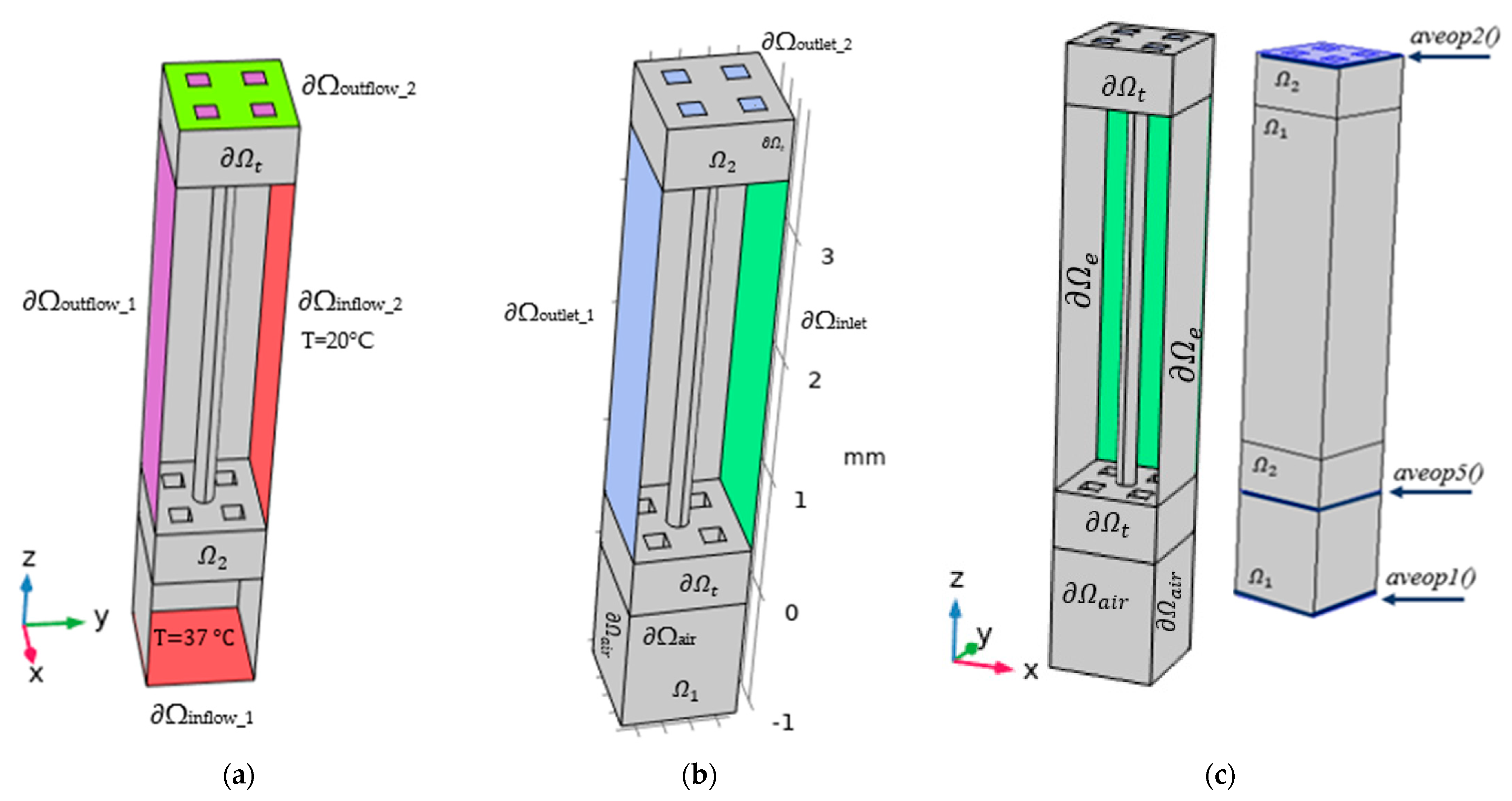
Moreover, the fluid velocity on the 3D textile surface ∂Ωt was set to zero. The constant temperature T = 37 °C was used as an inflow condition to simulate the heat temperature released by the skin surface ∂Ωinflow. On ∂Ωoutflow surface heat flux condition was applied that boundary condition requires heat transfer (h) coefficient that was obtained from the computational model described in Section 2.2.1. Figure 4a illustrates the positions of the boundary conditions for heat transfer on solids and fluids (.ht) interface for 1 cell. Figure 4b illustrates the positions of the boundary conditions for the laminar flow (.spf) interface. A Nonisothermal flow (.nitf) interface was used to combine the set of equations.
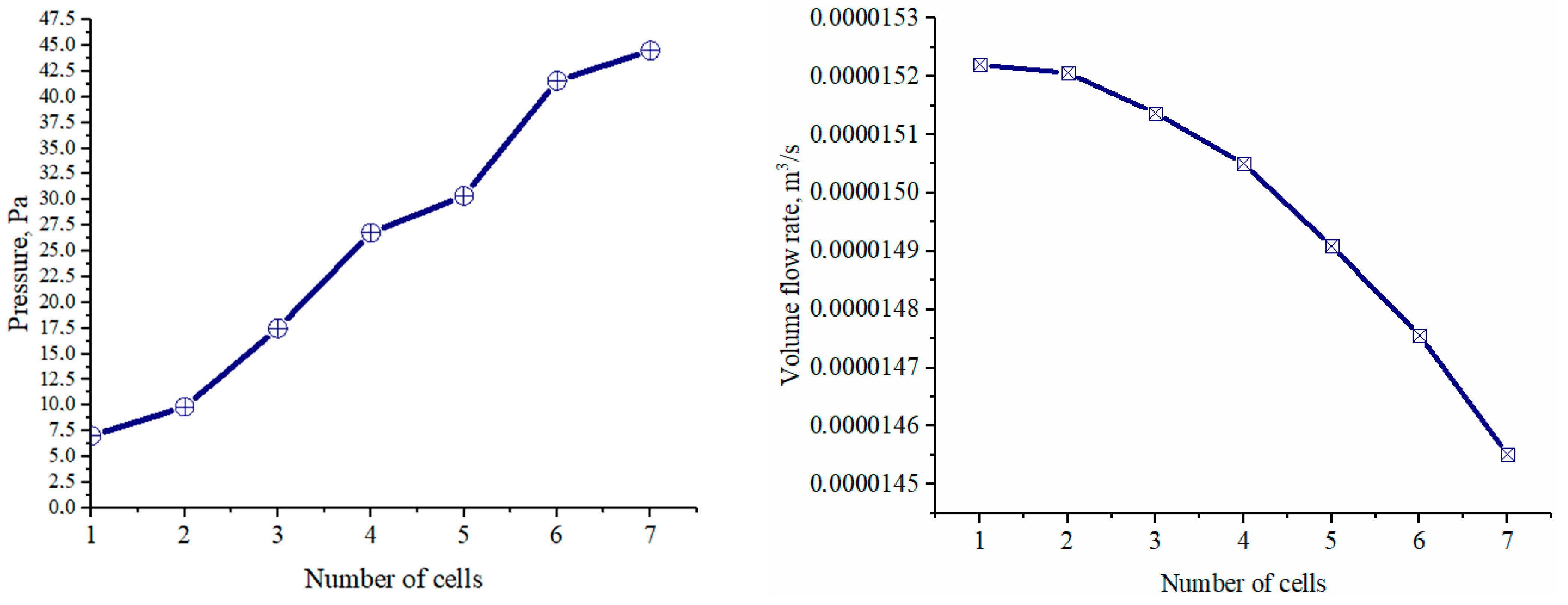
Numerical simulations were performed under these boundary conditions (see Table 2) which were adapted for different cell numbers (see Figure 3). The analysis demonstrated that at a given value of the inlet air flux rate the inlet pressure and the air flux rate are different depending on the number of cells. The larger number of cells increases the resistance to airflow; therefore, the inlet pressure also becomes larger at the same value of the inlet air flux rate. Simultaneously, the air flux rate in each cell also decreases because of the flux loss through the openings at the top of each cell. This enables to select the boundary conditions which could be suitable for a representative cell. The boundary conditions on the representative cell are based on the air flux difference between the right- and left-hand sides of a cell, see Figure 5. The values were taken from air fluxes between the boundaries of the 6th and 7th cells where the relationship of air flux against the number of cells is close to linear. Table 3 represents the updated boundary conditions that were used in further simulations. It should be noted that, on ∂Ωinlet the average volume flow rate of 0.000014716 m3/s was applied. This value was determined from the simulation that the computational domain consists of 6 cells. Moreover, on ∂Ωoutlet_1 the average volume flow rate was set to 0.000014552 m3/s and it was obtained from the simulation that the computational domain consists of 7 cells.

2.2.1. Determination of Thermal Resistance

The thermal resistance of textile fabrics experimentally might be evaluated using different standard test methods such as the tog test (BS 4745), clo test (ASTM D-1518), sweating-guarded hotplate (ISO 11092), and THL (ASTM F1868) [3]. In this subsection, a computational model that predicts the thermal resistance of textile structures is based on the sweating-guarded hotplate test method. The numerical prediction of the thermal resistance Rct was performed following standard LST EN 31902/ISO 11092:2014(en) [31]. ISO 11092 is usually referred to as the “skin model” and imitates the heat transfer through the skin [3]. The thermal resistance of textile structures is defined as the temperature difference between the two faces of a material (Tm and Ta), divided by the resultant heat flux H per unit area A in the direction of the gradient (see Equation (4)) [31]. The measurement of the thermal resistance of the fabric requires that the temperature of the measuring unit is 35 °C, the ambient air temperature is (20 ± 2) °C, and the relative humidity is (65 ± 5)% [31,41].
R c t = T m T a A H Δ H c R c t 0 ,
where Tm—mean temperature of the measuring unit K, Ta—air temperature in the test enclosure K, H—heating power W required to maintain the plate temperature at T = 35 °C, ΔHc—correction term for heating power is 0, and Rct0—the apparatus constant m2·K/W for the measurement of thermal resistance without sample [31,41].
The thermal resistance Rct coefficient was modeled according to the energy equation (see Equation (3)) [38]. On the inflow boundary, the temperature was set to T = 35 °C, and on the outflow boundary T = 20 °C. The computational domain is depicted in Figure 6. In this simulation, the air domain height is approximately equal to the textile domain height. The computational model was done under the assumption that the flow is stationary non-isothermal flow, and the heat exchange occurs due to conduction. During simulations, it was assumed that the 3D textile is made from polyester and the fluid is moist air. The moist air properties might be obtained from the literature [42] or interface Heat transfer in solids and fluids (.ht) using specific media that represent the region of a moist air domain. The thermal resistance Rct coefficient can be defined from Equation (5) [24] and the heat transfer h coefficient from Equation (6) [41]. In addition, the thermal resistance Rct coefficient in Comsol Multiphysics environment might be determined as (aveop1(T)-aveop2(T))/aveop1(ht.ntflux), where aveop1(), aveop2() are the average operators on surfaces ∂Ωinflow and ∂Ωoutflow, T—temperature, ht.ntflux denotes normal total heat flux [43].
R c t = T Q / A .
h = 1 R c t

2.2.2. Mesh Analysis

The finite element mesh represents a solution field. By increasing the number of mesh elements, a more accurate approximation and solution can be obtained. However, it takes more time and requires more memory to solve the problem [40].
In this study, the optimal mesh size was determined by evaluating and comparing the numerically predicted air permeability (AP) coefficient with experimental data from the literature [34]. The proposed computation model of the air permeability (AP) coefficient was built on the assumption that airflow is an incompressible Newtonian flow and has a low Re number. The computational model is based on the Navier–Stokes (see Equation (1)) [38] and Brinkman equations (see Equation (7)) [38], as well as the continuity Equation (see Equation (2)) [38], where ρ, μ, p, εp, k are the density, dynamic viscosity, pressure, porosity, and local permeability, respectively. The finite element model follows the ISO 9237:1995 (E) standard [35], where the pressure difference between the inlet and outlet boundaries is 200 Pa. A more detailed explanation of boundary conditions is presented in the research conducted by the authors of this article [36].
In order, to determine an optimal mesh five different meshes (extremely coarse, extra coarse, coarser, coarse, and normal) were taken into consideration. Then, the numerical solution of AP was compared with experimental data [34] taking into account computation time and relative error.
ρ ε p u u ε p = p I + μ ε p u + u Τ μ k 1 u .   i n   Ω 2

2.3. Development of a Micro-Scale Model

The computational model of the forced ventilation was built using COMSOL Multiphysics software. The interfaces of Laminar flow (.spf) and Heat transfer in solids and fluids (.ht) were applied. The approach of finite element analysis is depicted in Figure 7. Lagrange linear discretization was applied for the temperature, velocity, and pressure. Moreover, different mesh size was taken into account during finite element analysis.
The simulations were performed using the steady-state nonlinear solver. A simplified case of equations and pseudo code is presented below. Newton’s method is the most widely used technique for solving nonlinear equations. Given F : R n R n , F = f 1 , , f n T and the task is to find the solution to nonlinear systems of Equation (8) [44].
F x = 0 .
It should be noted that F is well defined and has continuous partial derivatives on an open set of R n , J(x) represents the Jacobian matrix [44]. It was assumed that solution x ¯ can be written as x ¯ = x0 + s, where x0 is some known guess of x, and s is a correction term. Given an initial estimation, x0 of the solution of Equation (8), Newton’s method considers, at each iteration, the approximation (see Equation (9)) [44]:
F x L k x F x k + J x k x x k .
Additionally, computes x k + 1 as a solution of L k x = 0 . This solution exists if J x k is non-singular. Therefore, an iteration of Newton’s method is described in Equation (10) [44] and Equation (11) [44].
J x k s k = F x k ,
x k + 1 = x k + s k .
In this study, Equation (10) [44] was solved using PARDISO solver, which was well documented in the literature [45]. The pseudocode of Newton’s algorithm is adapted from the literature [46] and presented below in Algorithm 1.
Algorithm 1. Pseudocode of Newton’s method for nonlinear equations.
1: Choose a starting guess x0 and accuracy є.
2: for k = 0, 1, 2, … do
3:             compute the correction s k . Solve J x k s k = F x k by the direct solver.
4:             update the solution guess x k + 1 = x k + s k .
5:             if s k < є then
6:                 stop.
7:             end if
8: end for
Note. For highly nonlinear problems, a damped update of the form x k + 1 = x k + α s k can be used, with 0 < α < 1 where α is a damping parameter.

2.4. The Macro-Scale Model

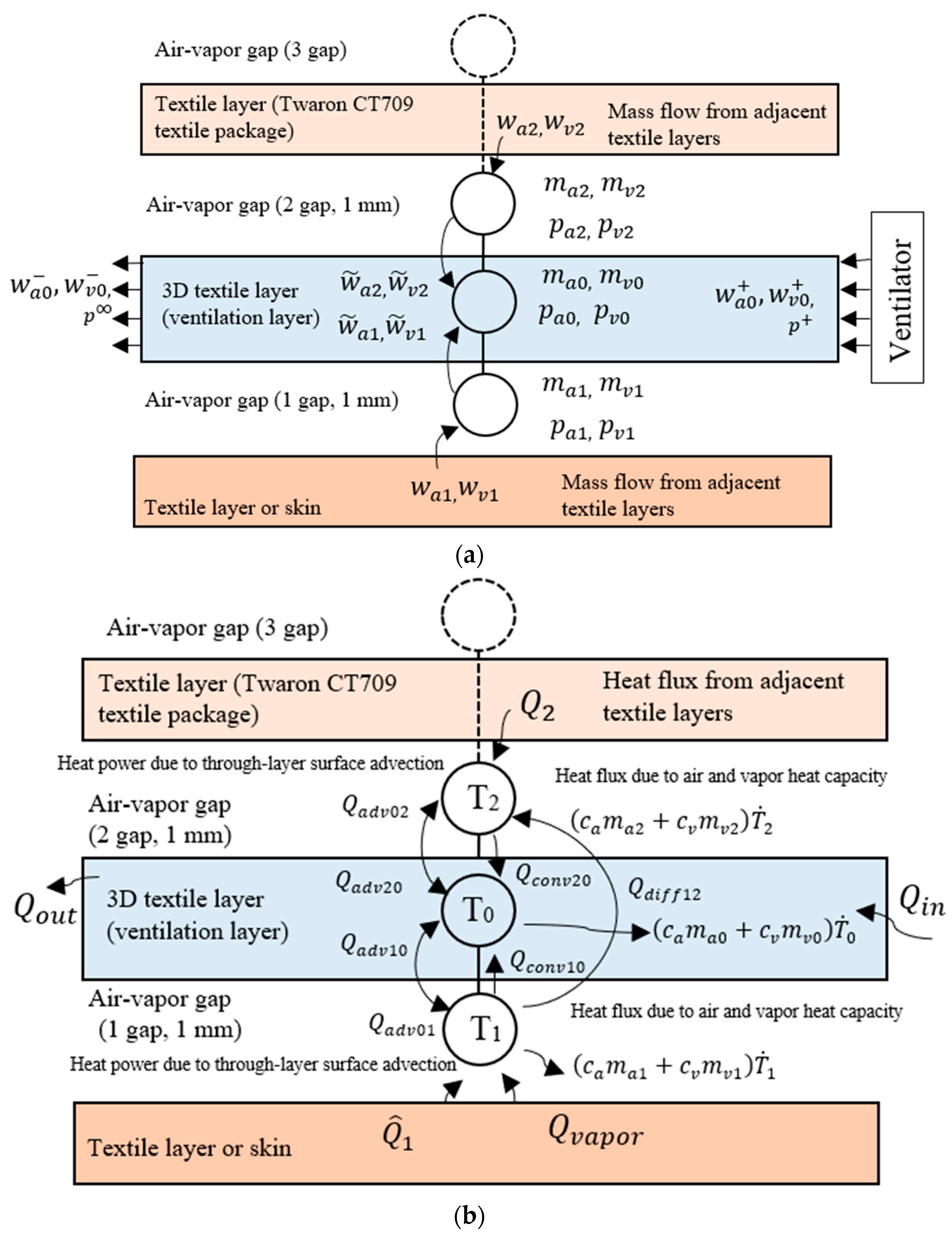
This subsection describes the finite element model of forced ventilation through the textile layer on a macro-scale. The proposed model is based on the literature [4,30]. Figure 8 illustrates the numerical scheme of water vapor and airflow, heat fluxes through a multilayered textile structure. Figure 8 was adapted from the literature [30]. The one-dimensional model consists of three nodes, two of which are positioned in the gaps at the bottom and top of the 3D textile layer, and the third node represents the inside of the ventilation layer [30]. The finite element model might be described by the structural Equation (12) [30]. That consists of the capacity matrix of the structure C U , vector of nodal variables U = m v 0 , m a 0 , T 0 , , m v 2 , m a 2 , T 2 . The final equation system of the proposed model in matrix form with the left-hand side capacity matrix of dimension 9 × 9 can be described by Equation (13) [30]. More details might be found in the literature [4,30]. The model was developed using Matlab software.
C U U ˙ = f U , t .
m a 0 m v 0 0 0 0 0 0 0 0 1 μ v 1 μ a p · h 0 A R T 0 2 0 0 0 0 0 0 c v T 0 c a T 0 c a m a 0 + c v m v 0 + c 3 D A 0 0 0 0 0 0 0 0 0 1 0 0 0 0 0 0 0 0 0 1 0 0 0 0 0 0 0 0 0 c a m a 1 + c v m v 1 0 0 0 0 0 0 0 0 0 1 0 0 0 0 0 0 0 0 0 1 0 0 0 0 0 0 0 0 0 c a m a 2 + c v m v 2 m ˙ v 0 m ˙ a 0 T ˙ 0 m ˙ v 1 m ˙ a 1 T ˙ 1 m ˙ v 2 m ˙ a 2 T ˙ 2 = = m a 0 w v 0 + m v 0 w a 0 + + m a 0 δ ~ p A p v 1 + p v 2 2 p v 0 m v 0 k ~ a A p a 1 + p a 2 2 p a 0 0 Q a d v 10 + Q a d v 20 α ~ A T 1 + T 2 2 T 0 c v w v 0 + + c v w ~ v 1 + c v w ~ v 2 + c a w a 0 + + c a w ~ a 1 + c a w ~ a 2 T 0 w ~ v 1 w ~ a 1 Q a d v 01 α ~ A T 1 T 0 α 3 D A T 1 T 2 w ~ v 2 w ~ a 2 Q a d v 02 α ~ A T 2 T 0 + α 3 D A T 1 T 2 + 0 0 c v w v 0 + + c a w a 0 + T w ^ ^ v 1 0 Q ^ 1 + c v w ^ ^ v 1 T h u m a n w v 2 w a 2 Q 2 .
The forced ventilation model in the macro-scale requires input parameters such as α ~ —heat transfer coefficient of the three-dimensional textile layer; α 3 D —heat transfer coefficient of the ventilation layer. These characteristics were determined using the micro-scale models described in previous sections.

3. Results and Discussion

3.1. Mesh Analysis

One of the most difficult aspects of developing computational models is determining the appropriate mesh size. In order, to obtain an optimal number of elements, computation time and accuracy were taken into account. This mesh analysis is essential for reducing computation time and demonstrating developed model accuracy. In this study, the relative error between the finite element solution and the experimental air permeability (AP) coefficient was determined. A RVE of Model 1_c was used and a mesh was applied to it. The numerical simulations were conducted with different meshes: extremely coarse, extra coarse, coarser, coarse, and normal, which represent 3194, 6249, 18,270, 57,795, and 125,512 elements, respectively. It should be noted that the minimum element quality was greater than 0.01, in order, to avoid convergence problems. It was found that using a coarser mesh relative error between the numerical solution and experimental data is 4.66%. Moreover, when coarse (57,795 elements) and normal (125,512) mesh are used, the relative error decreases to 0.25% and 0.16%, respectively. However, computation time increases from 9 s to 111 s (see Figure 9). Figure 9b, demonstrates that computation time vs. the number of elements increases according to the polynomial function. It was obtained that the coefficient of determination R-square is 0.9985. For further simulations, the coarse mesh was employed in the simplified geometry domain as the optimal mesh for numerical simulations.

3.2. Thermal Resistance Evaluation at a Micro-Scale

Numerical predictions of thermal resistance Rct and heat transfer h coefficients were determined for 3D textile structures corresponding to Model 1_e, Model 2_e, and Model 3_e. It was assumed that 3D textile is made from polyester and the fluid is moist air. Table 4 summarizes the determined thermal resistance Rct and heat transfer h coefficients. It was found that the heat transfer coefficient varies from 8.53 to 8.96 W/(K·m2). It might be noticed that the heat transfer coefficient slightly increases with the increased thickness. In the literature [30], the measured thermal resistance Rct and heat transfer h coefficients of 3D textile are presented and equal to 0.118 K·m2/W and 8.4746 W/(K·m2), respectively. However, the main differences may be due to differences in the height of samples, different space yarn configurations, initial material properties, and other factors. Figure 10 depicts temperature distribution through the height (z-axis) of Model 1_e. It should be noted that the heat transfer h coefficient corresponding to Model 3_e was used in a forced ventilation micro-scale model.

3.3. Combined Forced Ventilation Micro- and Macro-Scale Models

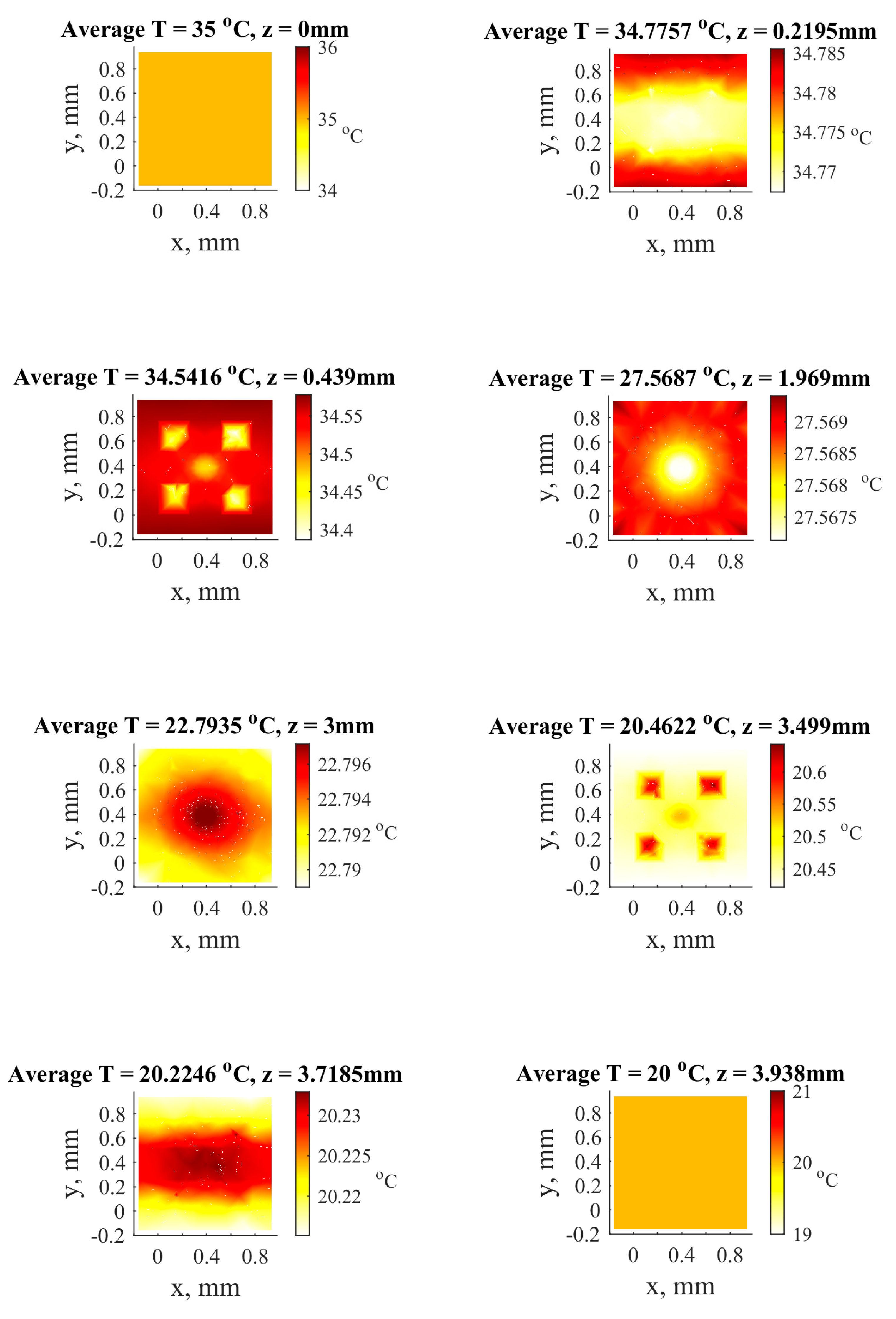
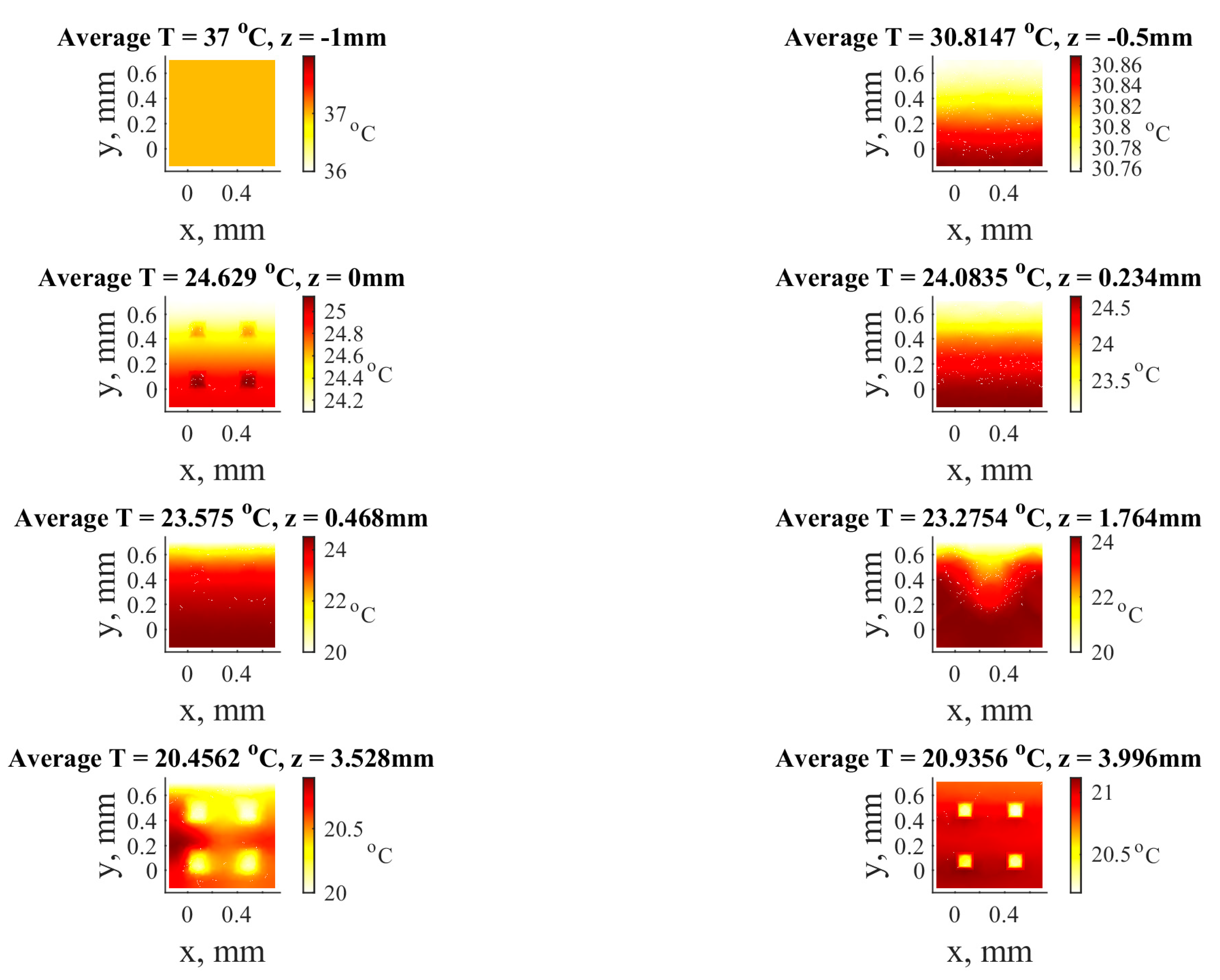
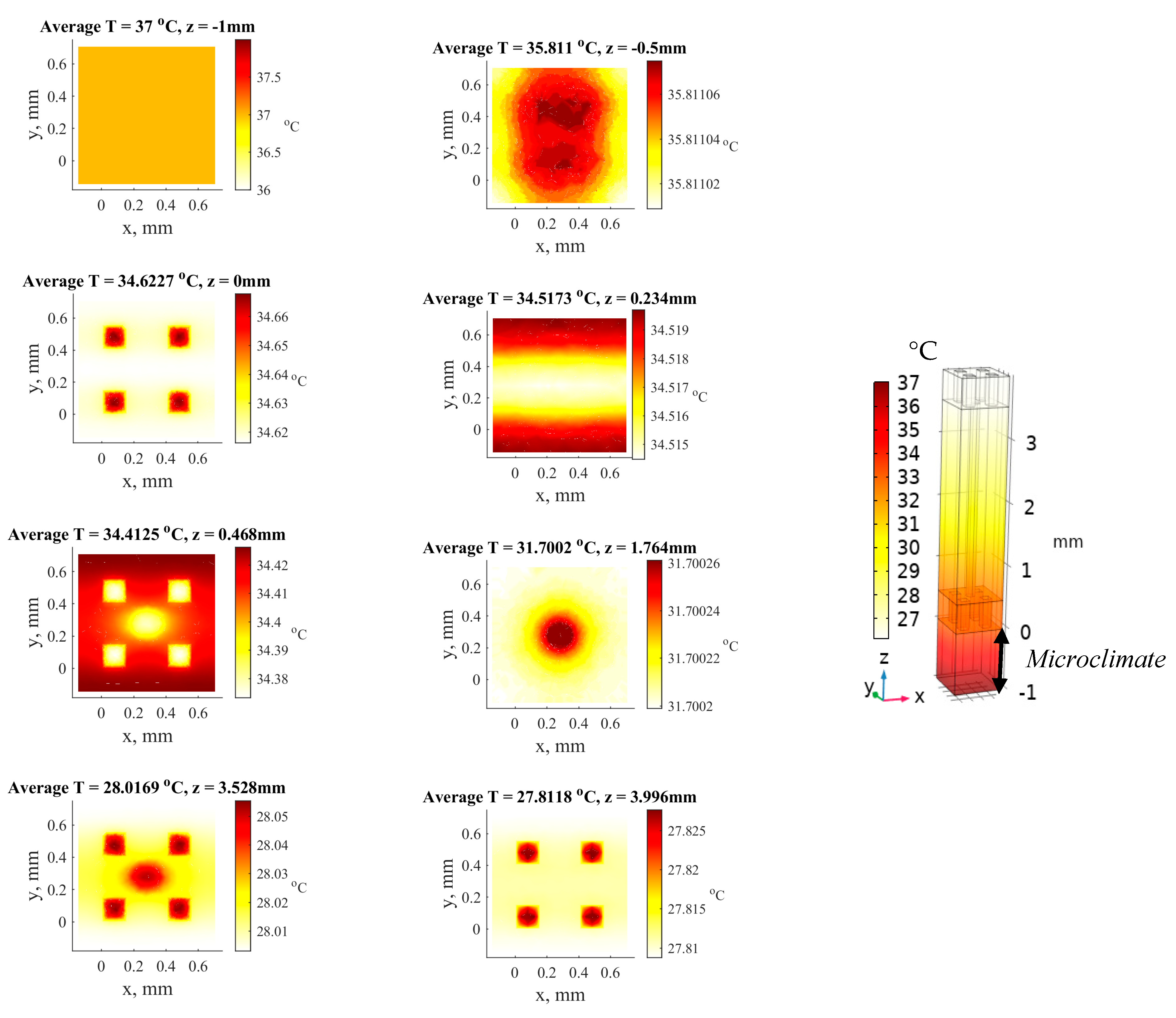
In Section 2.2, a forced ventilation model at a micro-scale was presented. The computational model allows for predicting the average temperature of the surface. The stationary temperature distributions via 3D textile structure, considering the flow rate of 0 and 0.000014716 m3/s were investigated. Figure 11 depicts the surface average temperature T °C and the position of the cut plane z, mm, when the flow rate is 0.000014716 m3/s. It was found that in the middle of microclimate (z = −0.5 mm), when the flow rate is 0 m3/s, the temperature is T = 35.81 °C, and with the flow rate 0.000014716 m3/s, T = 30.8147 °C. It was obtained that on ∂Ωoutflow (z = 3.996 mm) surface the temperature is T = 27.81 °C (no ventilation) and T = 20.93 °C (Qsv = 0.000014716 m3/s). Figure 12 depicts temperature distributions when the mass flow rate is zero. Moreover, a three-dimensional view of the object is presented. The main tendency is that temperature decreases due to increased mass flow rate.
Furthermore, the heat transfer h coefficients were determined. The effective heat transfer coefficients are summarized in Table 5. The hmicrolayer stands for heat transfer between the skin surface and the bottom of the textile layer. It was obtained by using average operators and follows Equation (6) which is equivalent to the expression aveop1(ht.ntflux)/(aveop1(T)-aveop5(T)). In addition, htotal is the total heat transfer coefficient between the skin and the outer layer, and it is determined from the expression: aveop1(ht.ntflux)/(aveop1(T)-aveop2(T)). It was obtained that an increase in the mass flow rate caused the rise of the heat transfer coefficient. On the other hand, it indicates a decrease in thermal resistance.
The computational model was built on the assumption that the flow is laminar and incompressible. As a result, the model is applicable in the range of small flow rates. Furthermore, 0.000014716 m3/s corresponds to a velocity of 7.1549 m/s, which can be considered a windy condition [47].
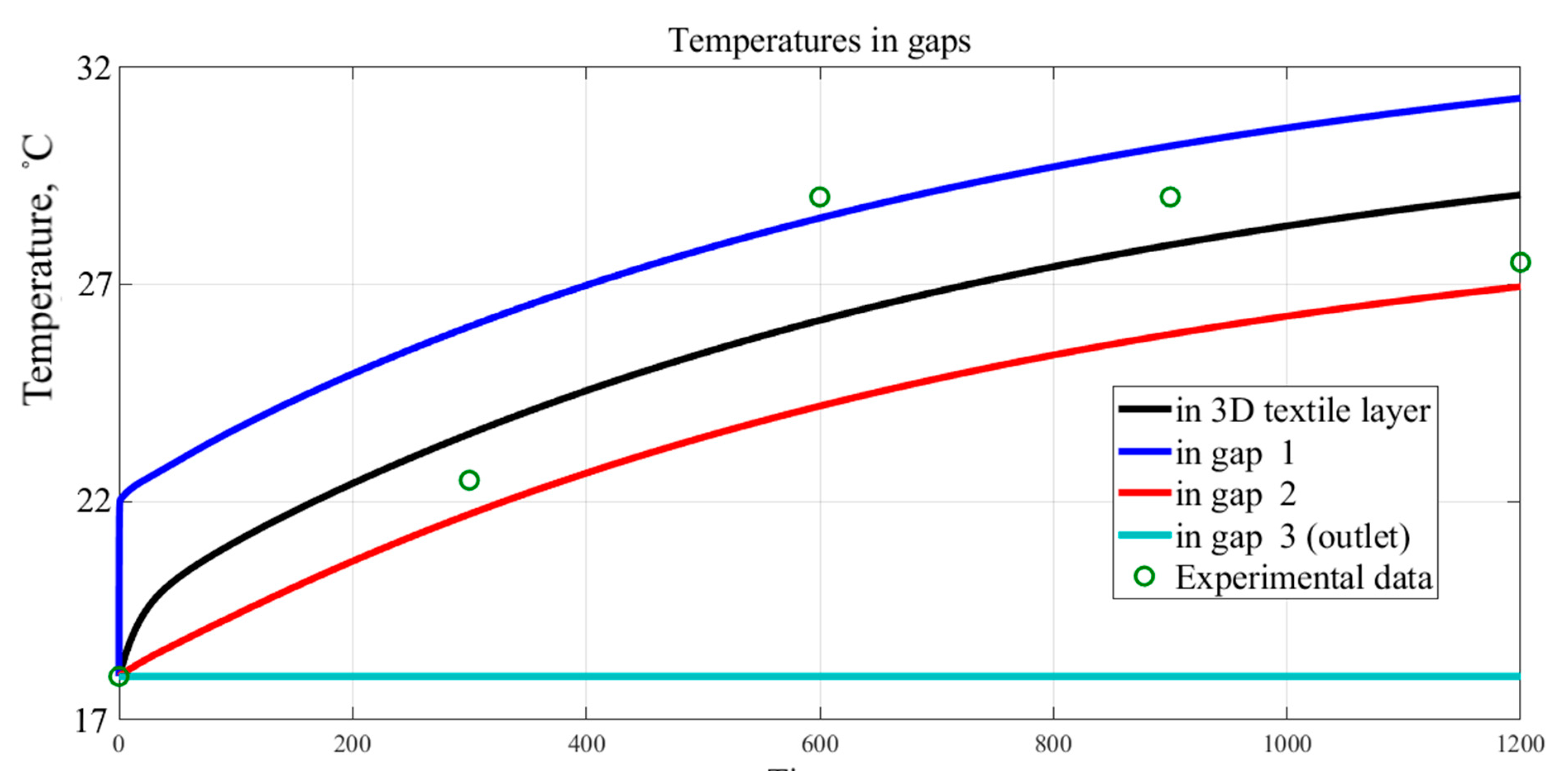
Finally, established effective heat transfer coefficients were applied to the finite element model on a macro-scale. In this investigation, α ~  = hmicrolayer = 25.603 W/(K·m2), α 3 D = htotal = 8.9646 W/(K·m2) were used from Table 4 and Table 5. Figure 13 depicts the obtained results. The temperature predicted numerically was compared to experimental data from the literature [4]. The determined results were quantitative and qualitatively similar to the experimental data. The mean absolute error between the finite element model and measurements in the 3D textile layer was approximately 1.29 °C.

4. Conclusions

The main purpose of this study was to develop combined micro- and macro-scale models to investigate heat and mass transfer through textile structures with additional ventilation. In this study, the wearing comfort properties such as air permeability, thermal resistance, and heat transfer coefficients might be predicted at a micro-scale. Moreover, computational models were extended to the forced ventilation models at a micro- and a macro-scale. The effective heat transfer coefficients of the ventilation layer from the micro-scale model were applied to a macro-scale model. Both finite element models simulate ventilation through the 3D textile in both steady-state and/or time-dependent modes. The numerical results demonstrated a good agreement with the experimental data presented in the literature. It was found that the mean absolute error of temperature between numerically predicted on a macro-scale and experimental data in the 3D textile layer was approximately 1.29 °C. However, the developed forced ventilation model at a micro-scale is valid for low mass flow rates.
The numerical simulations of heat and mass transfer through textile structures with additional ventilation were performed using COMSOL Multiphysics and Matlab software.
New technological developments in the field of textiles provide a wide spectrum of materials with different physical properties. For this reason, theoretical analysis of thermal comfort properties is essential for ensuring wearing comfort. The computational models proposed in this study can be used in the early stages of designing functional clothing such as protective clothing. Additionally, the proposed theoretical approach might be applied to other scientific and engineering purposes related to heat and mass transfer through three-dimensional structures.

Author Contributions

Conceptualization, R.B.; methodology, A.G. and R.B.; software, A.G., R.B.; validation, A.G., R.B. and A.A.; formal analysis, A.G.; investigation, A.G.; resources, A.A.; data curation, R.B.; writing—original draft preparation, A.G.; writing—review and editing, R.B. and A.A.; visualization, A.G.; supervision, R.B.; project administration, R.B.; funding acquisition, R.B. All authors have read and agreed to the published version of the manuscript.

Funding

This research received no external funding.

Data Availability Statement

Not applicable.

Conflicts of Interest

The authors declare no conflict of interest.

References

  1. Li, Y. The science of clothing comfort. Text. Prog. 2001, 31, 1–135. [Google Scholar] [CrossRef]
  2. Zhang, C.; Wang, F. Comfort Management of Fibrous Materials 31.2 Human Thermal Regulation and Heat Transfer; Wiley: Hoboken, NJ, USA, 2020; pp. 857–887. [Google Scholar]
  3. Tessier, D. Testing Thermal Properties of Textiles; Elsevier Ltd.: Amsterdam, The Netherlands, 2017. [Google Scholar]
  4. Barauskas, R.; Baltušnikaite, J.; Abraitiene, A.; Grinevičiute, D. Experimental investigations and finite element model of heat and moisture transfer in multilayer textile packages. Fibres Text. East. Eur. 2012, 95, 112–118. [Google Scholar]
  5. Angelova, R.A.; Kyosov, M.; Stankov, P. Numerical investigation of the heat transfer through woven textiles by the jet system theory. J. Text. Inst. 2019, 110, 386–395. [Google Scholar] [CrossRef]
  6. Das, T.; Das, A.; Alagirusamy, R. Study on thermal protective performance of thermal liner in a multi-layer clothing under radiant heat exposure. J. Ind. Text. 2022, 51, 8208S–8226S. [Google Scholar] [CrossRef]
  7. Goldstein, R.; Eckert, E.; Ibele, W.; Patankar, S.; Simon, T.; Kuehn, T.; Strykowski, P.; Tamma, K.; Heberlein, J.; Davidson, J.; et al. Heat transfer—A review of 2001 literature. Int. J. Heat Mass Transf. 2003, 46, 1887–1992. [Google Scholar] [CrossRef]
  8. Zhang, J.; Chauhan, S. Fast explicit dynamics finite element algorithm for transient heat transfer Jinao Zhang, Sunita Chauhan Department of Mechanical and Aerospace Engineering, Monash University, Wellington Rd, Clayton, Melbourne, VIC 3800, Australia. Int. J. Therm. Sci. 2019, 139, 160–175. [Google Scholar] [CrossRef] [Green Version]
  9. Udayraj; Talukdar, P.; Das, A.; Alagirusamy, R. Heat and mass transfer through thermal protective clothing—A review. Int. J. Therm. Sci. 2016, 106, 32–56. [Google Scholar] [CrossRef]
  10. Fan, J.; Luo, Z.; Li, Y. Heat and moisture transfer with sorption and condensation in porous clothing assemblies and numerical simulation. Int. J. Heat Mass Transf. 2000, 43, 2989–3000. [Google Scholar] [CrossRef]
  11. Xu, D.H.; Ge, M.B.; Zhang, H.L. Numerical solution of a dynamic model of heat and moisture transfer in porous fabric under low temperature. Int. J. Heat Mass Transf. 2013, 61, 149–157. [Google Scholar] [CrossRef]
  12. Li, Y.; Luo, Z.X. Physical mechanisms of moisture diffusion into hygroscopic fabrics during humidity transients. J. Text. Inst. 2000, 91, 302–316. [Google Scholar] [CrossRef]
  13. Li, Y.; Zhu, Q. A model of coupled liquid moisture and heat transfer in porous textiles with consideration of gravity. Numer. Heat Transf. Part A: Appl. 2003, 43, 501–523. [Google Scholar] [CrossRef]
  14. Madhu, M.; Kishan, N. Finite element analysis of heat and mass transfer by MHD mixed convection stagnation-point flow of a non-Newtonian power-law nanofluid towards a stretching surface with radiation. J. Egypt. Math. Soc. 2016, 24, 458–470. [Google Scholar] [CrossRef] [Green Version]
  15. Simões, N.; Tadeu, A.; António, J.; Mansur, W. Transient heat conduction under nonzero initial conditions: A solution using the boundary element method in the frequency domain. Eng. Anal. Bound. Elem. 2012, 36, 562–567. [Google Scholar] [CrossRef]
  16. Long, G.; Liu, Y.; Xu, W.; Zhou, P.; Zhou, J.; Xu, G.; Xiao, B. Analysis of Crack Problems in Multilayered Elastic Medium by a Consecutive Stiffness Method. Mathematics 2022, 10, 4403. [Google Scholar] [CrossRef]
  17. Gholamreza, F.; Su, Y.; Li, R.; Nadaraja, A.V.; Gathercole, R.; Li, R.; Dolez, P.I.; Golovin, K.; Rossi, R.M.; Annaheim, S.; et al. Modeling and Prediction of Thermophysiological Comfort Properties of a Single Layer Fabric System Using Single Sector Sweating Torso. Materials 2022, 15, 5786. [Google Scholar] [CrossRef] [PubMed]
  18. Acharya, J.; Dinda, A.; Bhanja, D.; Misra, R.D.; Nath, S. Influence of aging and body location on the thermal performance of firefighter’s clothing exposed to radiant heat source. Int. J. Therm. Sci. 2023, 184, 108024. [Google Scholar] [CrossRef]
  19. Lim, J.; Choi, H.; Roh, E.K.; Yoo, H.; Kim, E. Assessment of airflow and microclimate for the running wear jacket with slits using CFD simulation. Fash. Text. 2015, 2, 1–13. [Google Scholar] [CrossRef] [Green Version]
  20. Sun, Y.; Jasper, W.J. Numerical modeling of heat and moisture transfer in a wearable convective cooling system for human comfort. Build. Environ. 2015, 93, 50–62. [Google Scholar] [CrossRef]
  21. Santos, M.S.; Oliveira, D.; Campos, J.B.L.M.; Mayor, T.S. Numerical analysis of the flow and heat transfer in cylindrical clothing microclimates—Influence of the microclimate thickness ratio. Int. J. Heat Mass Transf. 2018, 117, 71–79. [Google Scholar] [CrossRef]
  22. Xu, P.; Kang, Z.; Wang, F.; Udayraj, U. A numerical analysis of the cooling performance of a hybrid personal cooling system (HPCS): Effects of ambient temperature and relative humidity. Int. J. Environ. Res. Public Health 2020, 17, 4995. [Google Scholar] [CrossRef]
  23. Siddiqui, M.O.R.; Sun, D. Computational analysis of effective thermal conductivity of microencapsulated phase change material coated composite fabrics. J. Compos. Mater. 2015, 49, 2337–2348. [Google Scholar] [CrossRef]
  24. Siddiqui, M.O.R.; Sun, D. Conjugate heat transfer analysis of knitted fabric. J. Therm. Anal. Calorim. 2017, 129, 209–219. [Google Scholar] [CrossRef]
  25. Joshi, A.; Psikuta, A.; Bueno, M.A.; Annaheim, S.; Rossi, R.M. Effect of movement on convection and ventilation in a skin-clothing-environment system. Int. J. Therm. Sci. 2021, 166, 106965. [Google Scholar] [CrossRef]
  26. Joshi, A.; Psikuta, A.; Bueno, M.A.; Annaheim, S.; Rossi, R.M. Analytical clothing model for sensible heat transfer considering spatial heterogeneity. Int. J. Therm. Sci. 2019, 145, 105949. [Google Scholar] [CrossRef]
  27. Renard, M.; Puszkarz, A.K. Modeling of Heat Transfer through Firefighters Multilayer Protective Clothing Using the Computational Fluid Dynamics Assisted by X-ray Microtomography and Thermography. Materials 2022, 15, 5417. [Google Scholar] [CrossRef]
  28. Codau, E.; Codau, T.C.; Lupu, I.G.; Raru, A.; Farima, D. Heat transfer simulation through textile porous media. J. Text. Inst. 2023, 114, 257–264. [Google Scholar] [CrossRef]
  29. Neves, S.F.; Campos, J.B.L.M.; Mayor, T.S. On the determination of parameters required for numerical studies of heat and mass transfer through textiles—Methodologies and experimental procedures. Int. J. Heat Mass Transf. 2015, 81, 272–282. [Google Scholar] [CrossRef] [Green Version]
  30. Barauskas, R.; Abraitiene, A. A model for numerical simulation of heat and water vapor exchange in multilayer textile packages with three-dimensional spacer fabric ventilation layer. Text. Res. J. 2011, 81, 1195–1215. [Google Scholar] [CrossRef]
  31. ISO 11092:2014(en) Textiles—Physiological Effects—Measurement of Thermal and Water-Vapour Resistance under Steady-state Conditions (Sweating Guarded-Hotplate Test). Available online: https://www.iso.org/obp/ui/#iso:std:iso:11092:ed-2:v1:en (accessed on 18 May 2023).
  32. Liu, Y.; Hu, H. Compression property and air permeability of weft-knitted spacer fabrics. J. Text. Inst. 2011, 102, 366–372. [Google Scholar] [CrossRef]
  33. Bargmann, S.; Klusemann, B.; Markmann, J.; Schnabel, J.E.; Schneider, K.; Soyarslan, C.; Wilmers, J. Generation of 3D representative volume elements for heterogeneous materials: A review. Prog. Mater. Sci. 2018, 96, 322–384. [Google Scholar] [CrossRef]
  34. Zupin, Ž.; Hladnik, A.; Dimitrovski, K. Prediction of one-layer woven fabrics air permeability using porosity parameters. Text. Res. J. 2011, 82, 117–128. [Google Scholar] [CrossRef]
  35. EN ISO 9237:1995; Textiles—Determination of Permeability of Fabrics to Air. Available online: https://www.iso.org/standard/16869.html (accessed on 18 May 2023).
  36. Gadeikytė, A.; Abraitienė, A.; Barauskas, R. Prediction of air permeability coefficient and water-vapor resistance of 3D textile layer. J. Text. Inst. 2022, 113, 396–404. [Google Scholar] [CrossRef]
  37. Gadeikytė, A. Multiscale Models and Algorithms for the Simulation of Heat and Moisture Transfer in Textile Structures. Ph.D. Thesis, Kauno Technologijos Universitetas, “Technologija”, Kaunas, Lithuania, 2022. [Google Scholar]
  38. Leal, L.G. Advanced Transport Phenomena; Cambridge University Press: New York, NY, USA, 2007. [Google Scholar]
  39. Elgeti, S.; Sauerland, H. Deforming fluid domains within the finite element method. Arch. Comput. Methods Eng. 2014, 23, 323–361. [Google Scholar] [CrossRef] [Green Version]
  40. COMSOL. COMSOL Multiphysics Reference Manual.Version: COMSOL 5.5; 2018. Available online: https://doc.comsol.com/5.5/doc/com.comsol.help.comsol/COMSOL_ReferenceManual.pdf (accessed on 18 May 2023).
  41. Sankauskaite, A.; Rubežiene, V.; Kubiliene, D.; Abraitiene, A.; Baltušnikaite-Guzaitiene, J.; Dubinskaite, K. Investigation of thermal behavior of 3D PET knits with different bioceramic additives. Polymers 2020, 12, 1319. [Google Scholar] [CrossRef] [PubMed]
  42. Tsilingiris, P.T. Thermophysical and transport properties of humid air at temperature range between 0 and 100 °C. Energy Convers. Manag. 2008, 49, 1098–1110. [Google Scholar] [CrossRef]
  43. Gadeikytė, A.; Sandonavičius, D.; Rimavičius, V.; Barauskas, R. Finite Element Analysis of Heat and Mass Exchange Between Human Skin and Textile Structures. Balt. J. Mod. Comput. 2022, 10, 159–169. [Google Scholar] [CrossRef]
  44. Martinez, J.M. Algorithms for solving nonlinear systems of Equations. In Algorithms for Continuous Optimization; NATO ASI Series (Series C: Mathematical and Physical Sciences); Springer Publishing: New York, NY, USA, 1994; Volume 434, pp. 81–108. [Google Scholar]
  45. Schenk, O.; Gärtner, K.; Fichtner, W. Scalable parallel sparse factorization with left-right looking strategy on shared memory multiprocessors. In Lecture Notes in Computer Science (Including Subseries Lecture Notes in Artificial Intelligence and Lecture Notes in Bioinformatics); Springer Publishing: New York, NY, USA, 1999; Volume 1593, pp. 221–230. [Google Scholar]
  46. Larson, M.G.; Bengzon, F. The Finite Element Method: Theory, Implementation, and Applications (Texts in Computational Science and Engineering); Springer: Berlin/Heidelberg, Germany; New York, NY, USA; Dordrecht, The Netherlands; London, UK, 2013. [Google Scholar]
  47. Shen, H.; An, Y.; Zhang, H.; Wang, F.; He, Y.; Wang, J.; Tu, L. 3D numerical investigation of the heat and flow transfer through cold protective clothing based on CFD. Int. J. Heat Mass Transf. 2021, 175, 121305. [Google Scholar] [CrossRef]
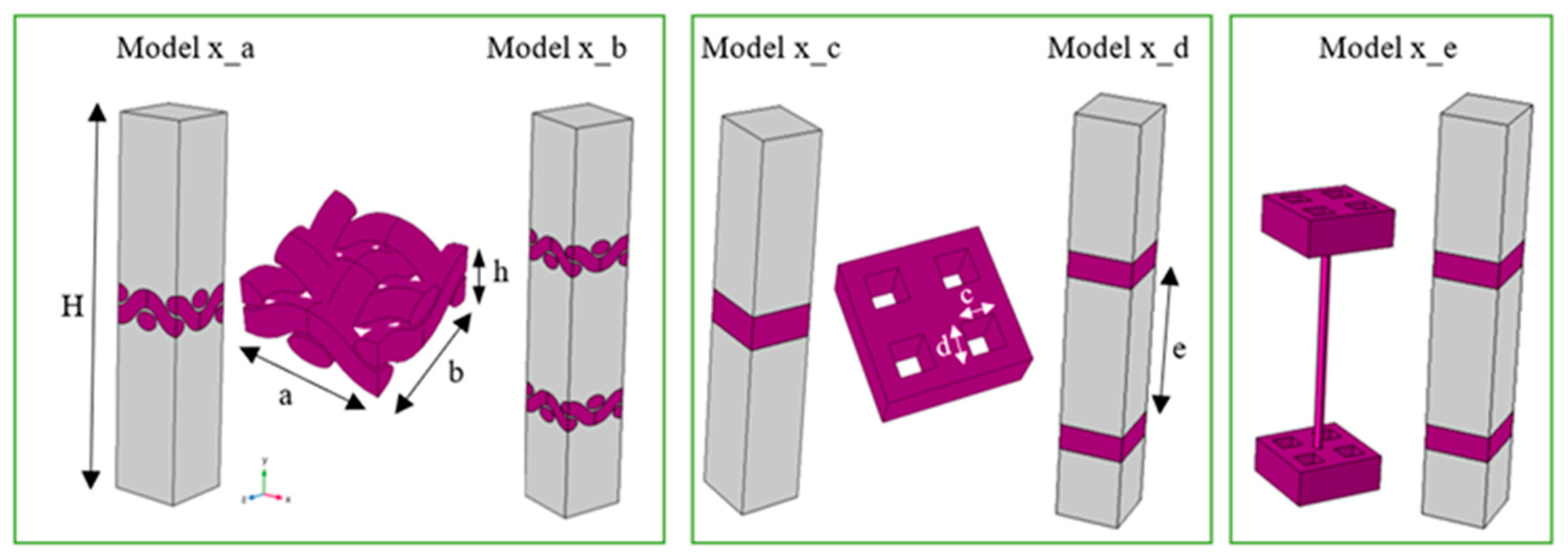
Figure 1. The general representation of RVE where x denotes the sample number, height of air domain—H, the thickness of the textile layer—h, length and width of domain a × b, length and width of pore c × d, and the distance between two layers of textile—e. The base units mm.
Mathematics 11 02532 g001
Figure 2. The primary heat and mass exchange scheme in an active cooler system [4].
Mathematics 11 02532 g002
Figure 3. The computational domains that consist of 1 to 7 cells.
Mathematics 11 02532 g003
Figure 4. (a) The boundary conditions of heat flow. (b) The boundary conditions of fluid flow. (c) Positions of average operators. The RVE with positions of boundary conditions (a,b), and average operators (c) is used in the postprocessing of outcomes. It should be noted that (a) depicts the boundary conditions used in the heat transfer on solids and fluids (.ht) interface; (b) depicts the boundary conditions applied to the laminar flow (.spf) interface.
Mathematics 11 02532 g004
Figure 5. The average pressure that was determined on surface ∂Ωinlet and average volume flow rate that was obtained on ∂Ωoutlet_1.
Mathematics 11 02532 g005
Figure 6. A RVE and boundary conditions of the thermal resistance model including the average operators.
Mathematics 11 02532 g006
Figure 7. The flowchart of the essential steps of finite element analysis.
Mathematics 11 02532 g007
Figure 8. A system of clothing–environment interaction, where heat and mass exchange simultaneously occurs. This figure represents the top, middle, and bottom nodes, respectively. m a 1 , m a 0 , m a 2 indicate the masses of air, m v 1 , m v 0 , m v 2 denote the masses of water vapor, w ~ v 1 , w ~ v 2 , w ~ a 1 , w ~ a 2 stands for the flow rates of water vapor and air, w a 0 + , w v 0 + the flow rates of air and water vapor supplied to the inlet of the 3D ventilation layer, w a 0 ¯ , w v 0 ¯ —the flow rates of air and water vapor supplied to the outlet of the 3D ventilation layer, w ^ ^ v 1 is an abbreviation for the water vapor mass flow rate generated by the skin, Q ^ 1 heat power produced by the skin, Q d i f f diffusive heat flux, Q a d v 01 , Q a d v 10 , Q a d v 02 , Q a d v 20 convective heat fluxes at both sides of the textile layer. (a) The mass flow rates of fluid. (b) The heat fluxes.
Mathematics 11 02532 g008
Figure 9. (a) Mesh size (number of elements) vs. air permeability (AP) coefficient and computation time. (b) Mesh size (number of elements) vs. computation time. (a) Demonstrates the convergence of the AP coefficients with an increasing number of elements. The squares depict the average AP and computation time that was evaluated from the numerical experiments, and the green dotted line and the area illustrate the experimental values of the average and standard deviation of AP. (b) Describes the relation between computation time and the number of elements (mesh size).
Mathematics 11 02532 g009
Figure 10. The temperature distribution through the z-axis of Model 1_e.
Mathematics 11 02532 g010
Figure 11. Temperature distribution at 0.000014716 m3/s flow rate, where T indicates the average temperature of the surface at a different z-axis position.
Mathematics 11 02532 g011
Figure 12. Temperature distribution at 0 mass flow rate, where T indicates the average temperature of the surface at a different z-axis position. A 3D plot of temperature distribution is shown on the right.
Mathematics 11 02532 g012
Figure 13. Temperature comparison between numerically predicted and experimental temperatures in a 3D textile layer.
Mathematics 11 02532 g013
Table 1. Air domain and textile layer structural parameters [37].
ModelLength and Width of Domain a × b (mm)Height of Air Domain H (mm)The Thickness of the Textile Layer h (mm)Length and Width of Pore c × d (mm)Distance between Two Layers of Textile e (mm)
Model 1_c1.1 × 1.1100.4390.263 × 0.263-
Model 1_e1.1 × 1.1100.4390.263 × 0.2633.06
Model 2_e0.98 × 0.98100.4380.195 × 0.1953.06
Model 3_e0.85 × 0.85100.4680.155 × 0.1553.06
Table 2. A list of the boundary conditions that were set in the ventilation model [37].
InterfaceSurfaceBoundary ConditionDescription
Fluid flowon ∂Ωinlet Ω ρ ρ s t u · n d b c d S = Q s v
Qsv- standard flow rate is 0.8 dm3/min.
Inlet boundary condition was used to apply the mass flow rate, where d b c stands for the fluid flow domain boundary thickness, the standard density is defined as ρ s t = p s t · M n R · T s t . In this investigation, the standard temperature Tst = 20 °C, M n a mean molar mass of the fluid (0.032 kg/mol), R—the universal molar gas constant, and p s —the standard pressure 1 [atm] [40].
on ∂Ωoutlet_1,
on ∂Ωoutlet_2.
p I + K n = p 0 n
p 0 p 0 , K = μ u + u T
p 0 = 0   Pa
Outlet on ∂Ωoutlet is a boundary where the fluid (net) outflows from the domain. The term p 0 stands for “suppress backflow”.
on ∂Ωt,
on ∂Ωair
u = 0 Wall condition: no-slip. The fluid velocity is zero. This boundary condition is used as the default.
on ∂Ωe u n = 0
K n K n n n = 0
K n = K n
Wall condition. The wall condition slip was applied on ∂Ωe surface.
Heat flowon ∂Ωinflow_1T = 37 °CTemperature. The inlet constant temperature was set to represent human skin temperature.
on ∂Ωinflow_2T = 20 °CTemperature. The inlet constant temperature was set to represent generated from the thermoelectric module.
on ∂Ωoutflow_1 n · q = 0 Outflow. In a model with convective heat transfer, this condition states that the only heat transfer occurring across the boundary is by convection. The temperature gradient in the normal direction is zero [40].
on ∂Ωoutflow_2 n · q = q 0
q 0 = h T e x t T
Heat flux. The h denotes a heat transfer coefficient. The h = 8.9646 W/(K·m2) was selected from Table 3, which was numerically predicted. T e x t is the external temperature. It was assumed that T e x t = 20  °C.
n · q = 0 Thermal insulation. This boundary condition is used as the default.
Table 3. A list of boundary conditions was updated and used in further simulations.
InterfaceSurfaceBoundary ConditionDescription
Fluid flowon ∂Ωinlet Ω ρ ρ s t u · n d b c d S = Q s v
Qsv- 0.000014716 m3/s.
Inlet boundary condition was used to apply the mass flow rate, where the standard density is defined as ρ s t = M n V m .   M n a mean molar mass of the fluid and V m —the standard molar volume.
on ∂Ωoutlet_1 u · t = 0
p I + K n = p g r a d n
Outlet on ∂Ωoutlet_1, the flow rate of 0.000014552 m3/s was applied.
Table 4. Numerically predicted thermal resistance Rct coefficient and heat transfer h coefficient.
ModelRct, K·m2/Wh, W/(K·m2)One-Layer Thickness, mmThe Height of the Model x_e, mm
Model 1_e0.117258.52870.4393.938
Model 2_e0.114558.72980.4383.936
Model 3_e0.111558.96460.4683.996
Table 5. Numerically predicted thermal resistance Rct coefficient and effective heat transfer coefficients.
Mass Flow Ratehmicrolayer, W/(K·m2)htotal, W/(K·m2)
No ventilation25.616.6368
With ventilation25.60319.747
Disclaimer/Publisher’s Note: The statements, opinions and data contained in all publications are solely those of the individual author(s) and contributor(s) and not of MDPI and/or the editor(s). MDPI and/or the editor(s) disclaim responsibility for any injury to people or property resulting from any ideas, methods, instructions or products referred to in the content.