Software Defect Prediction with Bayesian Approaches

Abstract

Software defect prediction is an important area in software engineering because it helps developers identify and fix problems before they become costly and hard-to-fix bugs. Early detection of software defects helps save time and money in the software development process and ensures the quality of the final product. This research aims to evaluate three algorithms to build Bayesian Networks to classify whether a project is prone to defects. The choice is based on the fact that the most used approach in the literature is Naive Bayes, but no works use Bayesian Networks. Thus, K2, Hill Climbing, and TAN are used to construct Bayesian Networks. On the other hand, three public PROMISE data sets are used based on McCabe and Halstead complexity metrics. The results are compared with the most used approaches in the literature, such as Decision Tree and Random Forest. The results from different performance metrics applied to a cross-validation process show that the classification results are comparable to Decision Tree and Random Forest, with the advantage that Bayesian algorithms show less variability, which helps engineering software to have greater robustness in their predictions since the selection of training and test data do not give variable results, unlike Decision Tree and Random Forest.

1. Introduction

The existence of software defects has been a great inconvenience and a challenge in software development and maintenance, having, therefore, a negative impact on software quality. Finding software that is free of defects is impossible, even though there is a careful process during software development. This is why software testing is a critical phase during the software development life cycle, since it is a way to prevent or even correct possible software failures before it is operable. However, the process involved in software testing is usually complicated, as it requires good planning and many resources [1].

Software defects significantly impact performance, quality, costs, and user satisfaction. Some of the more common impacts of having a lot of software defects include delays in product delivery, additional or unforeseen costs, poor user experience, loss of customer confidence, and even security issues. All these consequences have a direct impact on the quality of the software.

Given the negative impacts generated by detecting software defects in the last phases of software development, the area of software defect prediction (SDP) arises, “in which a prediction model is created in order to predict the future software faults based on historical data” [2]. Therefore, predicting defects is necessary to identify potentially defective modules in the software so that a software product that is efficient, reliable, and at a not-very-high cost can be obtained in a timely manner. If it is possible to identify modules prone to defects, monetary and human resources could be allocated to prevent unforeseen costs.

Developing a software defect prediction model is not an easy task. This is where artificial intelligence, using machine learning (ML) algorithms, can support software engineering for predicting software defects in the early stages.

Based on research conducted by Hammouri et al. in [2], where some classifiers based on machine learning algorithms such as Naïve Bayes (NB), Decision Trees (DT), and Artificial Neural Networks (ANN) are discussed for the prediction of software defects, it is considered that there are other alternatives that can give better results in terms of precision, such as algorithms based on Bayesian approaches, which “solve a variety of problems in various domains; from predicting a disease/treatment of a patient to analyzing genetic maps or expression analysis” [3].

On the other hand, Herzig et al. in [4] mention that, through manually examining seven thousand problem reports from the bug databases of five open-source projects, it was found that 33.8% of all reports were misclassified because they did not have defects, but instead they were referencing a new feature, update, or refactoring. Consequently, the prediction of software defects has been affected since it depends on the quality of the data to be evaluated. If these data are incorrect, it is impossible to reach a high percentage of accuracy in prediction. For all of the above, it seeks to explore the performance and precision of algorithms based on Bayesian Networks (little-explored algorithms) that allow more certainty to be given to software engineers when making estimates and delivering a quality product.

In a systematic literature review in [5], 38 studies were presented between 2016 and 2020 in software defect prediction to analyze the most-used classification approaches and algorithms in this area. In this study, it is presented that the most-used approaches are assembled algorithms such as Random Forest [6,7] followed by other algorithms such as AdaBoost [8] and Bagging [9], among others. At the same level as the previous approach, approaches based on Bayes’ theorem were also identified. However, all have used the Naive Bayes algorithm and its variants [7,10,11].

There are other approaches, such as Decision Trees; in particular, C4.5 is the algorithm that has been reported the most [10]. In addition, different simpler classifiers, such as Support Vector Machine [12,13,14], K-Nearest-Neighbor [14], and Logistic Regression [13,15], have been used.

More recently, other works have been found where they compare different approaches [16,17,18]. These comparisons are made mainly between the assembly methods where the classification is performed via multiple algorithms and methods with classical approaches. There are even works such as [19], where different versions of an algorithm such as Support Vector Machine (SVM) are experimented with.

1.1. Motivation

The motivation of this work is to benefit software engineers in the generation of more accurate and robust defect prediction models, that is, methods whose results are not sensitive to different training data. This is important as good defect prediction allows them to identify the areas and modules of the software most prone to bugs or defects. This helps development and testing teams focus their efforts on those critical areas, reducing the risk of defects spreading and affecting the overall functionality and quality of the software.

1.2. Problem Statement

As shown in the works in

Table 1. Summary and comparison of our research and current recent research (NR = Not reported, DT = Decision Tree, EM = Ensemble Methods, NB = Naïve Bayes, NN = Neural Networks, KNN = K-Nearest Neighbor, SVM = Support Vector Machine, LR = Logistic Regression and BN = Bayesian Network).

Ref	Year	Approaches Used	Bayesian Networks Use	Performance Analysis	Comparison with Other Similar Approaches or Variants	Comparison with Other Approaches
[6]	2019	DT, EM	NO	NO	YES	YES
[7]	2020	DT, EM	NO	NO	NO	YES
[9]	2020	EM	NO	YES	YES	NO
[10]	2018	NB, DT, EM, SVM	NO	NO	NO	YES
[11]	2020	NB, DT, NN	NO	YES	NO	YES
[12]	2020	DT, NB, LR, EM, SVM	NO	NO	NO	YES
[14]	2019	SVM	NO	YES	YES	NO
[15]	2018	EM, NN, DT	NO	NO	NO	YES
[16]	2022	LR, SVM, KNN, DT	NO	NO	NO	YES
[17]	2022	SVM, DT, KNN, NN, NB	NO	NO	NO	YES
[18]	2022	LR, DT, EM	NO	NO	NO	YES
[19]	2022	SVM	NO	YES	YES	NO
Our Research	2023	BN, EM, DT	YES	YES	YES	YES

, most of the works only report the best result. This is important because the machine learning algorithms used can be sensitive to training data and perform differently against test data. If the test data are similar to the training data, better results will be obtained. For this reason, it is necessary to report the performance of the classification algorithms. Therefore, not only is the precision of a classification algorithm sufficient, but it is robust to different data sets. Cross-validation procedures are commonly used to generate models with different training data from the data set and evaluate them with different test subsets of the data set not used for training.

Another situation that can be observed in Table 1 is that there are different versions of the same algorithm; however, the general version is usually reported. Lastly, when evaluating an algorithm with a specific approach (such as Decision Tree, Ensemble Methods, or KNN, among others), comparisons with other approaches are not reported in many cases. Finally, using Bayesian Networks was not found in any cited work, but the classic Naive Bayes algorithm was found. We speculate that the limited adoption of Bayesian Networks within software engineering may stem from a potential lack of familiarity with this particular approach. However, this approach has many advantages, as will be mentioned throughout this article, and we believe that it would be an excellent option to explore its use performance.

1.3. Contribution

The key contribution of our research is summarized below:

• In this paper, we empirically show the results of applying classification algorithms based on Bayes’ theorem not reported in the literature in software defect prediction, specifically, different ways of building Bayesian Networks. The above is to provide software engineers with other strategies to predict software defects in their projects.
• The choice of Bayesian Networks rests on the fact that it is not only enough to know the value of the class variable for software engineers and testers, but it is also important to know the characteristic that they should pay more attention to. Furthermore, some algorithms, such as KNN or Random Forest, do not express the variables that most impact the decision of the classification task.
• These tests were performed on the well-known public PROMISE repository to make the results repeatable and comparable.
• We perform a statistical comparison of the tests executed with a cross-validation method (10-fold as it is usually done in the literature) to know the performance of the algorithms compared with different training and test data. These comparisons allow us to know the best and worst results, that is, how variable their performance is.
• We also compare the methods proposed in the experimentation with two approaches mentioned in the literature, J48 (Decision Trees approach) and Random Forest (ensemble algorithms approach).
• The comparison in this paper does not include the precision metric since it only measures the number of well-classified records among the total tests. This is important since the class values of the data sets are unbalanced, and just using the precision metric would bias the results towards the class value that appears the most. We use metrics such as recall, accuracy, and F1-measure that measure different aspects of a model’s performance.
• With the results, a discussion is presented to balance the precision and robustness of the different methods tested.
• This work is important because the software defect prediction area allows developers and project leaders to know when the system can be released, reducing the use of unforeseen resources and improving the user experience through reducing the number of defects.

1.4. Paper Organization

This document is divided as follows. Section 2 presents related works that allow decisions to be made for the experimentation of this research. Section 3 presents our proposal. Section 4 describes the characteristics of the data sets used. Section 5 describes the experiments and evaluation form and analyzes the main results. Finally, Section 6 concludes and presents future work.

2. Related Work

The works mentioned in Section 1 helped us decide the focus of this research. First, although the Bayesian approach is one of the most frequently used, we found previous works using Bayesian Networks since Naive Bayes has practically been used, so we see an excellent opportunity to explore these approaches. Additionally, the approaches proposed in this study will be compared with the algorithms and approaches most used in the literature. It is decided to use an ensemble approach such as Random Forest and a Decision Tree such as C4.5.

Table 2. Summary of metrics and validations method reported in recent research (NR = not reported).

Ref	Data Set	Cross Validation	Best Approach	Accuracy	Recall	F1-Measure
[6]	CM1	10-fold	Random Forest/Sampling	NR	NR	0.92
[6]	JM1	10-fold	Random Forest/Sampling	NR	NR	0.85
[6]	KC1	10-fold	Random Forest/Sampling	NR	NR	0.87
[7]	CM1	10-fold	Random Forest	0.97	0.97	0.97
[7]	JM1	10-fold	Random Forest	0.81	0.81	0.77
[7]	KC1	10-fold	Random Forest	0.83	0.85	0.83
[8]	CM1	NR	Ada Boost	0.87	NR	NR
[8]	JM1	NR	Ada Boost	0.89	NR	NR
[8]	KC1	NR	Ada Boost	0.85	NR	NR
[14]	CM1	10-fold	Support Vector Machine	0.88	0.89	0.82
[14]	JM1	10-fold	Support Vector Machine	0.81	0.82	0.79
[14]	KC1	10-fold	Support Vector Machine	0.84	0.83	0.84
[16]	CM1	NR	Random Forest	0.86	NR	NR
[16]	JM1	NR	Random Forest	0.34	NR	NR
[16]	KC1	NR	Naive Bayes	0.77	NR	NR
[17]	CM1	NR	K-NN undersample	0.89	NR	NR
[17]	JM1	NR	SVM undersample	0.93	NR	NR
[17]	KC1	NR	K-NN undersample	0.96	NR	NR
[19]	CM1	NR	SVM-Linear	0.79	NR	NR
[19]	JM1	NR	SVM-RBF	0.88	NR	NR
[19]	KC1	NR	SVM-Linear	0.83	NR	NR

shows metrics used to evaluate the classifiers’ performance and their results, where the following stand out: precision, recall, F1-measure, accuracy, and area under curve. This is important because the best performance of an algorithm depends on the metric used, and it is important to evaluate it with different metrics since they measure different performances. In addition, some mitigate problems such as class imbalance or overfitting. For this reason, the most popular metrics were selected to evaluate the research results. However, as shown in Table 2, many related works only focus on describing the precision of a proposal with a single metric. This is somewhat suspicious since the nature of the data means that different metrics must be used according to the class, not just percentage accuracy.

Furthermore, it can be seen in Table 2 that many of the studies do not mention a model validation method. This is important because data selection for training and testing the models influences the results obtained.

3. Our Proposal

Although there are different algorithms for predicting software defects with a reasonable accuracy percentage, it is important to look for other classification alternatives that obtain a higher rate of software defect prediction accuracy. Thus, the algorithm should contribute positively to what impacts software reliability, quality, and high costs. Improving the accuracy of software defects implies, in turn, improving the performance of developers, reducing test times, and benefiting project managers in terms of resource allocation in a more efficient way. We focus on this approach as we highlight some advantages over other models.

The main reason to choose Bayesian Networks is their ability to model causal relationships between variables, which can help understand the relationships between features of a software product that influence whether it is prone to defects.

Secondly, according to the nature of Bayes’ theorem, this structure handles uncertainty in the data, which can be important when working with noisy (or outlier) or incomplete data.

Third, Bayesian Networks are flexible and can handle different types of variables, including continuous and discrete variables, which does not restrict the type of data obtained using software metrics.

Finally, unlike other machine learning algorithms (such as K-Nearest Neighbor or Random Forest), the structure can be interpreted. This is especially important because a software engineer can interpret, through a graph, the relationships between software attributes and pay attention to those that have a bad influence on a defective product.

3.1. Bayesian Approach

The Theorem of Bayes is a proposition used to calculate an event’s conditional probability. It was developed by the British mathematician and theologian Thomas Bayes. The main objective of this theorem is to determine the probability of an event compared to the probability of another similar event. In other words, it allows knowing the conditional probability of an event or occurrence determined as A given B, in which the probability distribution of event B given A is analyzed [20].

Bayes formula, also known as Bayes rule, determines the probability of an event. In the Bayes formula, three different probabilities are present, as is shown in Equation (1), where P(A) is the probability that represents a priori of an event A, P(A|B) is the probability that represents a posteriori of an event A and P(B|A) is the probability of an event B based on the event A information.

$$P(A|B)=\frac{\left(P\right(B\left|A\right)\ast P\left(A\right))}{P\left(B\right)}$$

(1)

3.2. Bayesian Networks

Bayes’ theorem is the foundation for the classifier known as the Bayesian Network. A Bayesian Network is a graphical model that shows variables (usually called nodes) in a data set and the probabilistic or conditional dependencies between them. A Bayesian Network can present the causal relationships between the nodes; however, the links in the network (also called edges) do not necessarily represent a direct cause-and-effect relationship.

On the other hand, Bayesian Networks are a type of probabilistic model that uses Bayesian inference for probability calculations. Bayesian Networks aim to model conditional dependency and causality through representing conditional dependency utilizing edges in a directed graph. Through these relationships, the inference about the random variables in the graph can be made efficiently using factors.

This classifier was selected because it is a compact, flexible, and interpretable representation of a joint probability distribution. It is also valuable for knowledge discovery since directed acyclic graphs represent causal relationships between variables [21]. Additionally, this model represents essential information regarding how the variables are related, which can be interpreted as cause–effect relationships. 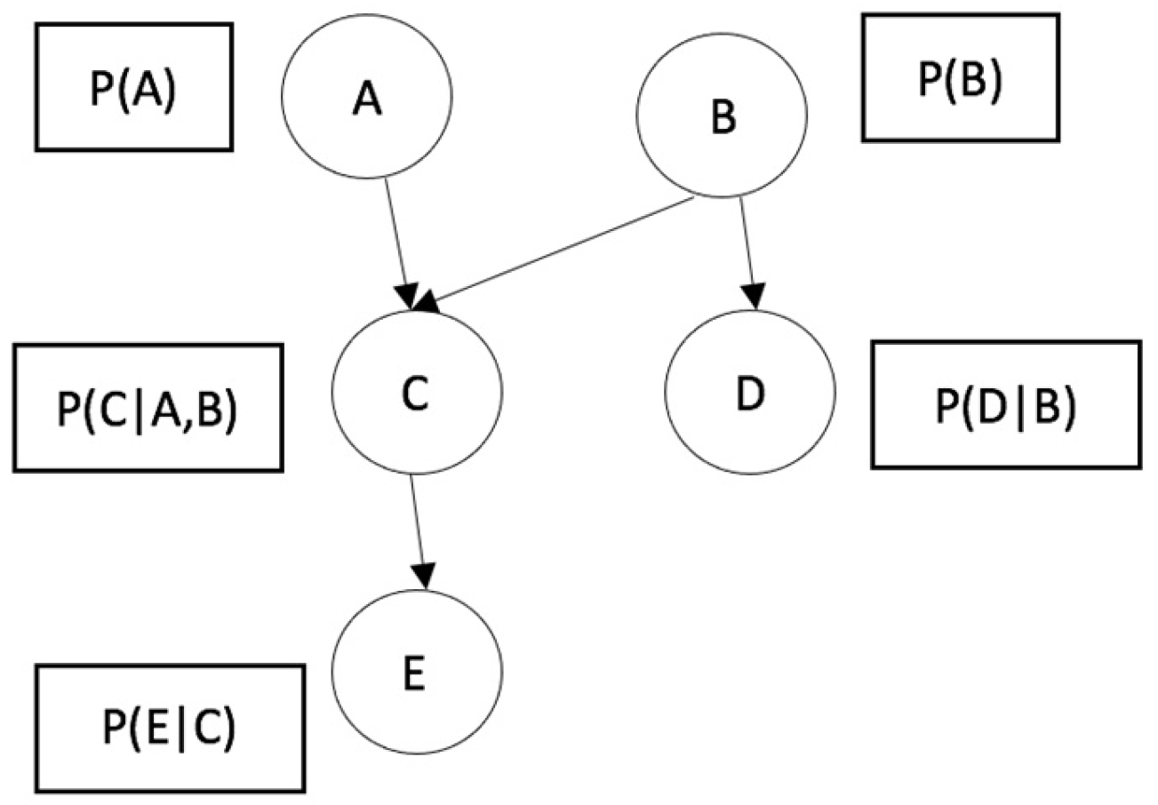Figure 1 shows the structure of a Bayesian Network as a directed acyclic graph. This structure reflects the relationship between the variables that represent conditional probabilities. For example, variable C is conditional on variables A and B.

However, there is no single way to generate a Bayesian Network, and the way to initialize and build it will depend on the results obtained. For this reason, three methods of building a Bayesian Network are proposed to apply to the problem of software defect prediction are presented below.

3.3. TAN

This algorithm, also known as a Tree Augmented Naïve Bayesian Network, is a Bayesian Network that consists of building a dependency tree between the variables to be predicted and which in turn are children of the class variable. Therefore, the probability of these variables will be calculated through applying Bayes’ theorem based on the probability of the class variable [22]. In conclusion, that assumes conditional independence between all variables given the class variables through allowing the predictor variables to depend on each other. Figure 2 shows how TAN builds a Bayesian Network, where the variable class has no parents, and the features (attributes) have the variable class and, at most, one other attribute as parents.

3.4. Hill Climbing

Hill Climbing is an optimization algorithm starting with a randomly generated Bayesian Network [23]. The algorithm randomly adds or eliminates relationships for each node or feature, calculating the probability of each node that makes up the network from the joint probability of the class variable. The algorithm chooses the optimal network with the best quality, eliminating those that do not reach its level. The score function typically used for Bayesian Networks is the log-likelihood function, which measures the probability of the observed data given the network structure and parameters. In other words, it measures how well the network predicts the data as is shown in Equation (2), where S is the score, G is the network structure, D is the data, X_i is the i-th variable, and Pa_i is the set of parents of X_i in G.

$$\mathrm{S}\left(\mathrm{G},\mathrm{D}\right)=\sum (\log \left(P\right(X_i\left|P{a}_i\right)\left)\right)-\sum (\log \left(P\left(X_i\right)\right))$$

(2)

3.5. K2

The K2 algorithm is a heuristic search that starts with the simplest possible network, a network without edges, and assumes that the nodes are ordered [24]. This algorithm adopts the idea of the greedy algorithm as the most traditional structure-learning algorithm [25]. K2 automates the process of learning the Bayesian Network structure, which means that a great deal of expert knowledge in the problem domain is not required. For each variable in the problem, the algorithm adds to its parent set the node with the lowest probability, leading to a maximum increase in quality corresponding to the quality of the measure chosen in the rating process. This process is repeated until the quality is not increased or a complete Bayesian Network is reached.

Based on these three approaches to generate a Bayesian Network, it is proposed to evaluate its performance in the data sets mentioned below.

4. Data Sets

The data sets used to evaluate the selected algorithms were taken from the PROMISE repository [26]. The reason these data sets were chosen is because they are public. These data sets are made public to foster repeatable, verifiable, refutable, and/or improvable predictive models of software engineering. In addition, PROMISE is one of the most used repositories for predicting software defects, according to the results obtained in the RSL.

Table 3. Distribution of classes by data set.

Data Set	Number of Instances	Distributions of Class (Defects)
		False	True
CM1	498	90.16%	9.83%
JM1	10,885	19.35%	80.65%
KC1	2109	15.45%	84.54%

shows the selected data sets with their number of instances and distribution of defect classes.

CM1 is a NASA spacecraft instrument written in “C” language, JM1 is written in “C” and is a real-time predictive ground system, and KC1 is a “C++” system implementing storage management for receiving and processing ground data. The discrete class variable indicates “the system has defects” or “No defects.”

The data sets have 21 explanatory variables or features. As it is shown in

Table 4. Distribution of attribute types.

Type of Attributes	Number of Metrics
Line of Code	5
McCabe measure	3
Base Halstead measure	4
Derived Halstead measure	8
Branch count	1
Total	21

, the features are divided into categories and described below.

4.1. McCabe Metrics

McCabe argued that code with complicated pathways is more error prone. His metrics, therefore, reflect the pathways within a code module [27].

Cyclomatic complexity is based on counting a program’s number of individual logical paths. To calculate software complexity, Thomas McCabe used graph theory and flow. In order to find the cyclomatic complexity, the program is represented as a graph, and each instruction contains a graph node. The possible paths of execution from an instruction (node) are represented in the graph as an edge.

According to the PROMISE repository, McCabe metrics are a collection of the three software metrics shown in

Table 5. McCabe metrics.

ID	Attribute	Value Type
1	V(g): cyclomatic complexity	numeric
2	Ev(g): essential complexity	numeric
3	Iv(g): Design complexity	numeric

.

4.2. Halstead Metrics

Halstead proposed a precise way of measuring a program’s size [28]. To do this, he considered that the code comprises units that called operators and operands, similar to the tokens that a compiler can distinguish in that code [29]. Additionally, these operators and operands do not always contribute equally to complexity. It is necessary to consider, in addition to the total number of elements, that is, operands and operators, the number of these that are different, that is, the program’s language.

Table 6. Halstead metrics.

ID	Measure Type	Attribute	Value Type
1	Base	Unique operators	numeric
2	Base	Unique operands	numeric
3	Base	Total operators	numeric
4	Base	Total operands	numeric
5	Derived	N (operators + operands)	numeric
6	Derived	Volume	numeric
7	Derived	Program length	numeric
8	Derived	Difficulty	numeric
9	Derived	Intelligence	numeric
10	Derived	Effort to write a program	numeric
11	Derived	Time to write a program	numeric
12	Derived	Halstead metric	numeric

shows the base and derived attributes of Halstead metrics.

4.3. Complementary Metrics

Five of the remaining six metrics refer to lines of code, and one to branch count.

Table 7. Complementary metrics.

ID	Measure Type	Attribute	Value Type
1	McCabe	Line count of code	numeric
2	Halstead	Line count	numeric
3	Halstead	Comment lines count	numeric
4	Halstead	Blank lines Count	numeric
5	Halstead	Code and Comment	numeric
6	-	Branch count	numeric

shows the characteristics of the last metrics, where it can be seen that for the code line count, one is also proposed by McCabe and four by Halstead. The branch count is taken from the flow graph.

4.4. Preprocessing Data

Once we have the data, we only check for missing data. Although outliers were identified in the data sets, since we did not collect the data, we decided not to remove them as we are unsure if they were capture errors or atypical data (outliers). This is a disadvantage of taking public data captured by other people since we do not have access to the projects.

5. Experiments and Results

This section presents the method for validating models in the experimentation, the metrics used, and the most significant results obtained when evaluating these Bayesian approaches in the PROMISE defect prediction data sets. All experiments were conducted on a platform using Weka 3.9.6, which can run on a Windows 10 Operating system with an Intel Core i7 3.6 Ghz and 8 GB RAM.

Table 8. Setup of the experimental parameters in Weka software.

Parameter	Value	Search Algorithm
Batch size	100	All
Score Type	MDL	All
Random order	False	K2
Init as Naïve Bayes	True	K2
Use Arc Reversal	False	Hill Climbing
Markov Blanket Classifier	False	K2 and Hill Climbing

describes the parameters used for the experiments so that these results can be reproducible. Some configuration parameters are not applicable to all search algorithms.

5.1. Cross-Validation

Cross-validation is a technique used in machine learning and statistics to evaluate the performance of a model on data that were not used during training. Cross-validation was selected because it ensures instances of the faulty class in every test set, thus reducing the probability of classification uncertainty [30]. The instances are divided into “folds,” and in each evaluation, the instances of each fold are taken as test data and the rest as training data to build the model. The calculated errors will be the average of all runs.

The experiments designed in the literature were reviewed to select the number of folds, as shown in Section 2. All of them used 10-fold cross-validation. Therefore, ten folds were chosen to evaluate a similar way to them.

5.2. Model Evaluation Metrics

The literature review found that when classification algorithms have been evaluated in the area of software defect prediction, the most-used metrics are accuracy, recall, and F1-measure. All of them are based on the confusion matrix shown in

Table 9. Confusion matrix structure.

Predicted	Actual
	Class X	Class Y
Class X	TP	FP
Class Y	FN	TN

, where TPs are True Positives, FPs are False Positives, FNs are False Negatives, and TPs are True Negatives. The confusion matrix is shown because, based on the values of this matrix, the model validation metrics, explained in the following subsections, are built. With this, the values with the best results will be on the main diagonal of the confusion matrix.

The metrics described below are widely used in different fields to evaluate the results of prediction models, as explained in [31].

Accuracy: This metric is the ratio of the results (both TP and TN) among the total number of instances examined. The best precision is 1, while the worst precision is 0. Accuracy is calculated as shown in Equation (3).

$$ACC=\frac{(TP+TN)}{TP+TN+FP+FN}$$

(3)

Precision: Calculated as the number of correct positive predictions divided by the total number of positive predictions. The best precision result is 1, while the worst is 0. Precision is calculated as shown in Equation (4). We can measure the quality of the machine learning model in the classification task with precision.

$$\mathit{Precision}=TP/(TP+FP)$$

(4)

Recall: It is calculated as the number of positive predictions divided by the total number of positives (wrong and well-classified). Recall tells us about the quantity that the machine learning model is able to identify. The best recall result is 1, while the worst is 0. The recall is calculated as shown in Equation (5).

$$\mathit{\text{Recall}}=\frac{TP}{TP+FN}$$

(5)

F1-measure: Defined as the weighted harmonic mean of precision and recall. In general, it combines precision and recall measures into a single measure to compare different machine learning algorithms against each other. F1-measure is calculated as shown in Equation (6).

$$F1-\mathit{\text{Measure}}=\frac{2\ast \mathit{\text{Recall}}\ast \mathit{\text{Precision}}}{\mathit{\text{Recall}}+\mathit{\text{Precision}}}$$

(6)

The proposed algorithms were also compared against two more commonly used algorithms in the literature (Decision Tree and Random Forest). For this work, the highest results obtained by the classifiers within each data set were considered. The results of the evaluation of the algorithms are shown in the following subsections according to metric and data set.

5.3. Accuracy Results

Table 10. Accuracy descriptive statistics for CM1 data set.

Algorithm	Max	Min	Mean	Median	Standard Deviation
K2	0.9183	0.898	0.9016	0.9	0.564
Hill Climbing	0.9183	0.84	0.9010	0.9	0.8353
TAN	0.92	0.76	0.8649	0.8775	4.07

,

Table 11. Accuracy descriptive statistics for JM1 data set.

Algorithm	Max	Min	Mean	Median	Standard Deviation
K2	0.8079	0.7904	0.8043	0.8062	0.45
Hill Climbing	0.8079	0.7904	0.8043	0.8062	0.45
TAN	0.8239	0.7840	0.8063	0.8069	0.76

and

Table 12. Accuracy descriptive statistics for KC1 data set.

Algorithm	Max	Min	Mean	Median	Standard Deviation
K2	0.8483	0.8436	0.8454	0.8436	0.22
Hill Climbing	0.8862	0.8142	0.8514	0.8530	1.53
TAN	0.8815	0.7962	0.8385	0.8388	1.88

show the performance of the K2, Hill Climbing, and TAN algorithms through descriptive accuracy statistics for each data set. In these tables, little variability is observed in the results of the ten folds. Likewise, the results between these three algorithms are very similar.

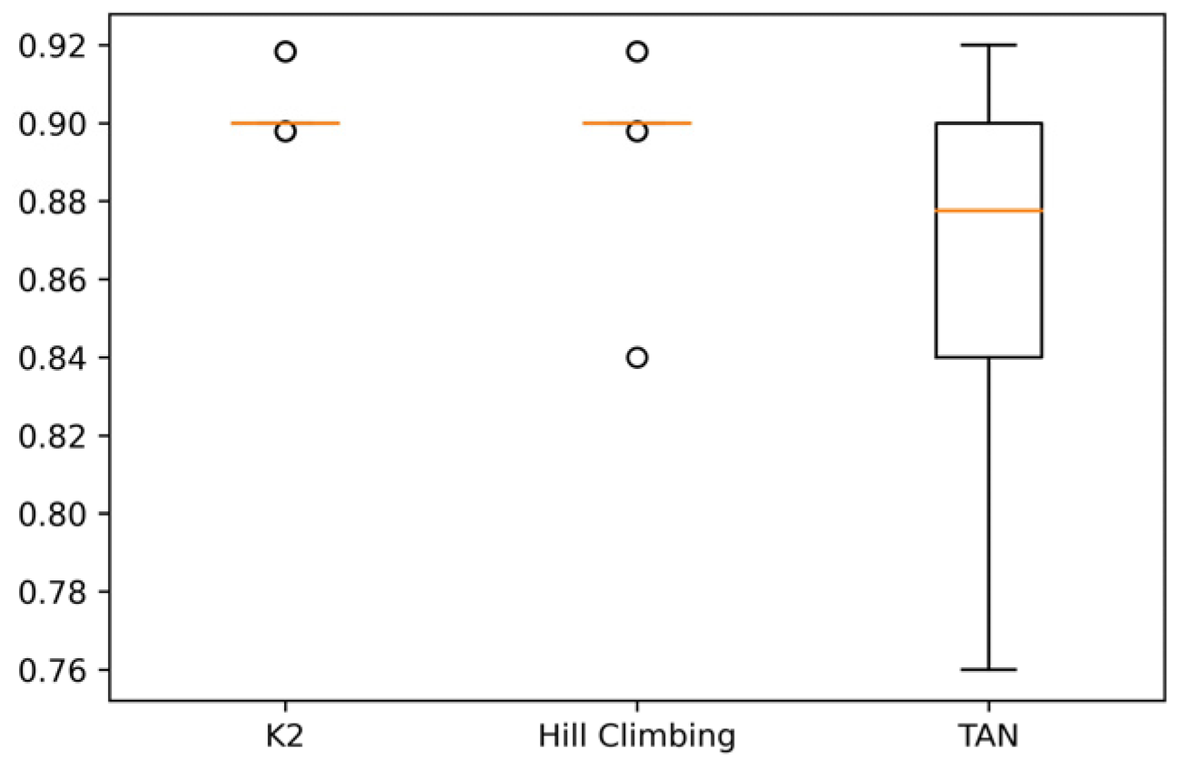
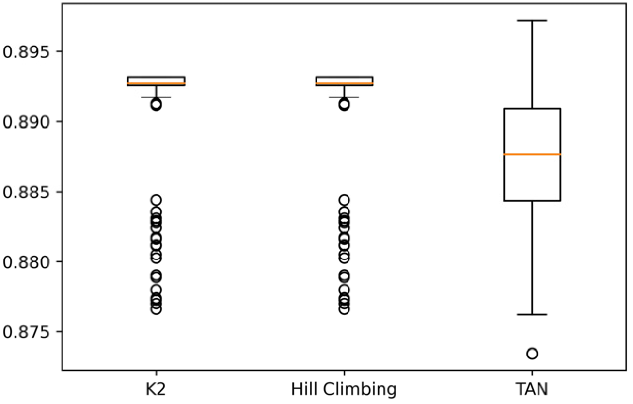
Figure 3, Figure 4 and Figure 5 show the variability of cross-validation runs for each data set. Figure 3 shows that accuracy with the K2 and Hill Climbing algorithms does not change in each run. In the case of the TAN algorithm, a significant variation is observed, indicating greater variability in the results when classifying the data with this approach. In Figure 4, it can be seen that, similar to the CM1 data set, in the JM1 data set, the K2 and Hill Climbing algorithms have little variability, which implies that these algorithms generate the same results with the data set, regardless of the projects used for training and testing. On the other hand, the TAN algorithm generates highly variable results. Finally, in Figure 5, it can be seen that in the KC1 data set, TAN is the algorithm with the most variability in accuracy. However, there is also variability with K2 and Hill Climbing, unlike the CM1 and JM1 data sets. From Figure 5, it is also concluded that the choice of data used for training and testing the KC1 data set influences a better or worse precision to classify the data.

Table 13. Accuracy results for the different data sets with other approaches.

Algorithm	CM1		JM1		KC1
	Best Accuracy	Standard Deviation	Best Accuracy	Standard Deviation	Best Accuracy	Standard Deviation
K2	0.9183	0.563	0.8079	0.454	0.8483	0.225
Hill Climbing	0.9183	0.835	0.8079	0.454	0.8862	1.526
TAN	0.92	4.077	0.8236	0.767	0.8815	1.887
Decision Tree	0.94	2.865	0.8170	0.886	0.8957	1.904
Random Forest	0.94	2.084	0.8382	0.808	0.9004	1.547

shows the comparison of the accuracy among the proposed algorithms with other classifiers, such as Decision Tree and Random Forest, where it can be seen that these last two obtained a higher percentage of accuracy than the Bayesian classifiers. However, the standard deviation they obtained is also higher. This is important since cross-validation indicates that their results have significant variability, and their results are not constant. With JM1, the results by classifiers are more balanced. It is important to mention that, in this evaluation, the TAN classifier obtained a higher result than the Decision Tree classifier, but Random Forest is still the highest. Finally, with the KC1 data set, it can also be seen that Decision Tree and Random Forest are the highest.

5.4. Recall Results

Table 14. Recall descriptive statistics for the CM1 data set.

Algorithm	Max	Min	Mean	Median	Standard Deviation
K2	1	1	1	1	0
Hill Climbing	1	0.93	0.93	1	0.006
TAN	1	0.82	0.94	0.95	0.046

,

Table 15. Recall descriptive statistics for the JM1 data set.

Algorithm	Max	Min	Mean	Median	Standard Deviation
K2	1	0.92	0.98	1	0.02
Hill Climbing	1	0.92	0.98	1	0.02
TAN	0.96	0.92	0.94	0.94	0.009

and

Table 16. Recall descriptive statistics for the KC1 data set.

Algorithm	Max	Min	Mean	Median	Standard Deviation
K2	1	1	1	1	0
Hill Climbing	1	0.93	0.96	0.96	0.01
TAN	0.98	0.89	0.94	0.94	0.01

show the performance of the K2, Hill Climbing, and TAN algorithms through descriptive recall statistics for each data set. The performance in this metric is more stable than accuracy and has better results, with K2 being the best because it reaches a higher recall and practically zero standard deviation.

Figure 6 shows the boxplot diagrams of recall in the CM1 data set for each algorithm, and it can be seen that for K2 and Hill Climbing, a box is not created because they do not change in each execution, unlike TAN, where there is more significant variability between their results; therefore, a box is created.

In Figure 7, where the experiment was carried out with the JM1 data set, it can be seen that, unlike the experiment with the CM1 data set, the data obtained via K2 and Hill Climbing already have a small variability. On the other hand, TAN continues to have more significant variability among its results.

Finally, Figure 8 shows that with the K2 algorithm, there are no variations between its results, and 100% (equivalent to 1) is obtained in recall. On the other hand, Hill Climbing also reaches 100%, but it does have variations in its results.

To conclude, the recall results runs with the Decision Tree and Random Forest algorithms were also compared. In

Table 17. Recall results for the different data sets with other approaches.

Algorithm	CM1		JM1		KC1
	Best Recall	Standard Deviation	Best Recall	Standard Deviation	Best Recall	Standard Deviation
K2	0.9183	0.563	0.8079	0.454	0.8483	0.225
Hill Climbing	0.9183	0.835	0.8079	0.454	0.8862	1.526
TAN	0.92	4.077	0.8236	0.767	0.8815	1.887
Decision Tree	0.94	2.865	0.8170	0.886	0.8957	1.904
Random Forest	0.94	2.084	0.8382	0.808	0.9004	1.547

, it can be seen that in the CM1 data set, the Bayesian algorithms obtained a better result than the other approaches and even have a lower standard deviation; their results are not distributed over a wide range of values. Even K2 obtained a value in the standard deviation of 0, and in recall 1, similar to Hill Climbing and TAN, with a difference in their standard deviation. With the JM1 data set, there is already variability of the Bayesian approaches, but they reach a higher recall than Decision Tree and Random Forest. Finally, they exhibit the same behavior in KC1, with little variability and better results for the Bayesian algorithms.

5.5. F1-Measure Results

Table 18. F1-measure descriptive statistics for CM1 data set.

Algorithm	Max	Min	Mean	Median	Standard Deviation
K2	0.95	0.94	0.94	0.94	0.003
Hill Climbing	0.95	0.91	0.94	0.94	0.004
TAN	0.95	0.86	0.92	0.93	0.024

,

Table 19. F1-measure descriptive statistics for JM1 data set.

Algorithm	Max	Min	Mean	Median	Standard Deviation
K2	0.89	0.87	0.89	0.89	0.005
Hill Climbing	0.89	0.87	0.89	0.89	0.005
TAN	0.89	0.87	0.88	0.88	0.004

and

Table 20. F1-measure descriptive statistics for KC1 data set.

Algorithm	Max	Min	Mean	Median	Standard Deviation
K2	0.91	0.91	0.91	0.91	0.001
Hill Climbing	0.93	0.89	0.91	0.91	0.008
TAN	0.93	0.88	0.90	0.90	0.011

show the performance of the K2, Hill Climbing, and TAN algorithms through descriptive F1-measure statistics for each data set. Although in no case is a value of 1 reached, the low variability of this metric can be appreciated for Bayesian algorithms, so it is concluded that in most cases, we will obtain similar values regardless of the data used for testing or training.

Figure 9, Figure 10 and Figure 11 show the variability of F1-measure with each algorithm in the cross-validation process. Figure 9 shows the minimum variability with K2 and Hill Climbing. However, in Figure 10, it can be seen that although there is little variability, there are outliers in K2 and Hill Climbing. Finally, in Figure 11, although there are no outliers, K2 continues to have the most consistent results.

In

Table 21. F1-measure results for the different data sets with other approaches.

Algorithm	CM1		JM1		KC1
	Best F1-M	Standard Deviation	Best F1-M	Standard Deviation	Best F1-M	Standard Deviation
K2	0.9574	0.003	0.8931	0.005	0.9179	0.001
Hill Climbing	0.9574	0.004	0.8931	0.005	0.9368	0.008
TAN	0.9574	0.024	0.89.72	0.004	0.9336	0.011
Decision Tree	0.9677	0.011	0.8934	0.005	0.9405	1.904
Random Forest	0.9677	0.016	0.8934	0.005	0.9405	1.547

, it can be seen that the results do not vary much between the Bayesian algorithms and Decision Tree and Random Forest. Yet, unlike recall, neither reaches a value of 1. However, Bayesian algorithms, compared to Decision Tree and Random Forest, are more constant and therefore have less variability, which helps the reliability of Bayesian algorithms in all data sets.

6. Conclusions and Future Work

The main objective of this research was to contribute to the software defect prediction field, with little-explored classification approaches in the area of software engineering. To carry out this research, the use of Bayesian Networks was proposed as an opportunity to improve defect prediction since these approaches are not found in the literature. In this research, cross-validation experiments were carried out to validate prediction models, and the results were compared with the metrics to evaluate the performance of algorithms using metrics such as accuracy, precision, recall, and F1-measure.

When analyzing the results, it can be observed that there is significant variability between them. This variability is because the data sets that were used to carry out the evaluations—that is, CM1, JM1, and KC1 taken from the PROMISE repository—are not balanced data sets, and this causes an imbalance when carrying out the experiments. Therefore, it is also of interest for future work to carry out the experiments using algorithms that allow balancing the classes.

As can be seen in the results, the search algorithms to initialize a Bayesian Network with Hill Climbing and K2 have less variability in the values of their evaluation metrics. This allows us to conclude greater robustness and independence of the data selection. TAN is the approach that, in all the experiments, had the most significant variability with the metrics. This variability depends on the structure of the network that is formed from the training data. TAN uses a dependency tree to capture the relationships between the variables in the Bayesian Network, as shown in Figure 2. This dependency is usually linear between the variables. If there are non-linear or complex dependencies between the variables, TAN may have difficulty capturing them adequately. The choice of training data influences the classification results.

According to the analysis of the results obtained, it is concluded that although the three selected Bayesian algorithms did not significantly exceed those found in the literature, Random Forest being the algorithm with the highest results, the values of the metrics used are comparable. However, Bayesian algorithms show less variability in the results, which benefits the classifications through being robust to data selection for training or testing. This can be explained since Random Forest depends on the selection of random samples, and these samples are suitable for making an accurate classification.

Therefore, it is suggested to use Bayesian algorithms since the results are comparable to Decision Tree and Random Forest, but Bayesian approaches will deliver consistent results with little variability regardless of the data selected for training or testing.

In future work, it is proposed to compare these Bayesian approach results with other ensemble classifiers (besides Random Forest). Ensemble classification algorithms combine multiple simpler classification models, intending to obtain a more accurate and robust prediction. One of the most common ensemble classification methods is Gradient Boosting, which is a method that builds a classification model in the form of a weighted combination of weaker classification models, usually Decision Trees. Another common ensemble classifier is Bagging, which is similar to Random Forest, but it differs in that Bagging allows sampling with replacement. It enables the same example to appear multiple times in the data set used to train each model. In short, ensemble classification methods are useful for combining multiple simpler models to improve the accuracy of predictions. At the same time, Bayesian Networks are models that provide a form of probabilistic reasoning. That is, they explicitly show the relationship between variables. The choice between both approaches depends on the specific problem, the available data, and the objectives of the analysis. With this future work proposal, it would be possible to find out if it is worth investing in more complex algorithms that result in the accuracy of prediction of software defects.

Finally, although one of the objectives of this study was to compare the performance between different machine learning approaches (Decision Trees, ensemble algorithms, and those based on Bayes’ theorem), these machine learning techniques could be compared with other approaches such as estimation based on analogy, where previously completed projects similar to the one that wants to be estimated are selected. Another option could be to compare it to “expert judgment”, where experts in the area of software estimation make estimates based on experience.