Abstract
This paper aimed to investigate the cornering characteristics of a Regional Haul Steer II, RHS 315/80 R22.5 truck tire traveling on a dry, hard surface using the Finite element analysis (FEA). This research was carried out using commercial Finite Element software and Pam-Crash in an Explicit Environment. A finite element truck tire model was developed to apply the tire terrain cornering condition. The concentrated loads and boundary conditions for the rim and wheel were applied to the model. The rubber material was defined using the Mooney–Rivlin model. The truck tire cornering operating conditions, including three different speeds with respect to various positive slip angles, were investigated. Several simulations were repeated at various operating conditions, including three different inflation pressures and three different vertical loads. Subsequently, the tire lateral force was computed using the local and global frame coordinates. Additionally, the self-aligning moment was extracted from the tire cross-section at each operating condition. Finally, a comparison between the simulation results showed that the tire lateral force was highly sensitive to the variation of the slip angles at the higher domain, and also that the tire inflation pressure, regardless of the speed, was considered to be one of the main parameters directly affecting the tire-cornering properties.
MSC:
74S05
1. Introduction
Pneumatic tires are the main components of light and heavy vehicles because they are objective to support the weight of a vehicle on its front and rear axles. Furthermore, the mechanical characteristics of these pneumatic tires play an important role in determining the accurate vehicle response properties, particularly when it comes to the vehicle dynamics field and control. Moreover, the handling performance is considerably affected by the tires of the vehicle. Therefore, truck tires have a significant effect on the performance of the truck under various operating conditions. In a cornering maneuver, the tire-cornering force is the lateral force that is generated due to the slip angles, which results in the tire’s steering from the direction of the wheel heading. In addition, tire lateral force is directly related to the lateral deformation of the tire due to the slip angles [1]. During cornering maneuvers, tires develop another force in the direction of the sliding surface, which is defined as the side force . While the cornering force and side force are usually not collinear, as shown in Figure 1 [2], it should be noted that, at the cornering maneuver, these two forces (the cornering force and the side force) develop a moment called the self-aligning moment, which is expressed as Equation (1).
Figure 1 shows an illustration of the pneumatic trail of a steered tire headed with a slip angle . The lateral distance (the compression of the tread elements at the contact length) or the offset between the cornering force and applied side force to the tire is called the pneumatic trail, . Since the (mechanical) pneumatic trail would vary with different tire slip angles, consequently, it has a significant effect on the final value of the tire self-aligning moment [3].

Figure 1.
Pneumatic trail [4].
The self-aligning moment is considered to be one of the primary restoring moments that acts on the Z-axis to realign a tire into its original position [2]. Based on Figure 2, the tire rolls on the road surface at the cornering maneuver, with respect to the slip angle, and the first principle of the tire, according to the vehicle control, is to generate the self-aligning moment about the Z-axis to realign the tire, due to the lateral force that has already been generated due to the existence of the slip angle and the steering of the direction of travel. Moreover, the self-aligning moment is one of the moments that plays a key role in the cornering performance of a tire, especially in heavy vehicles. Therefore, it is very important to predict the precise behavior of these tires, especially truck tires, at different slip angles to optimize the fuel consumption and achieve a better handling. On the other hand, optimizing the cornering behavior of truck tires has some environmental advantages that lead to a significant effect on lowering air pollution and decreasing exhaust and NOx emissions. In addition, a short literature review will be presented in the next section.
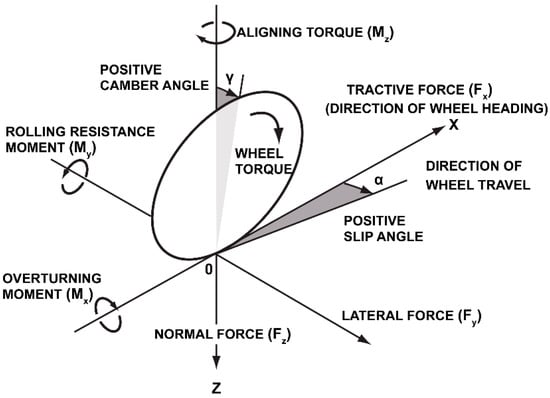
Figure 2.
SAE tire axis and terminology [2].
Several researchers have put great effort into the investigation of tire–terrain interactions, including cornering characteristics, using the Finite Element Analysis. The objective of these studies has been considerably focused on precise predictions of the tire lateral force and the self-aligning moment from the tire section at the tire-cornering maneuvers, according to the study of different parameters. In 2018, El-Sayegh et al. [5] presented a novel method for predicting the cornering characteristics of truck tires traveling on wet surfaces using Smoothed-Particle Hydrodynamics (SPH). The tire and wet road characteristics were determined using the Finite Element Method (FEM) and validated with experimental data that revealed a good agreement between the simulation and experimental tests using the Pam-Crash software. The FEM-SPH simulations were performed under several operating conditions, however, the speed of the tires was kept low due to stability concerns. However, the tires utilized in this study were simplified smooth tires and no rubber material analysis was indicated.
In 2014, Anupam et al. [6] studied cornering maneuvers for a pneumatic tire 185/60 R15 using the Finite Element package in Abaqus. The tire–road interaction was modeled with the real asphalt pavement and the cornering friction coefficient was computed.
In 2012, Oertel et al. [7] described a new method based on the nonlinear finite element method for estimate tire lateral force and self-aligning torque by implementing the kinematic theory and using the Euler method to calculate the tire forces and moments. In 2011, Nikola et al. [8] generated a finite element tire model based on a special CAD model in the Abaqus software. In their studies, an FE tire model rolling on the drum was simulated to predict the self-aligning torques. The simulation results were compared to their experimental tests and they showed an adequate accuracy by considering the friction coefficient of the tire tread.
In 2006, Ghoreishy et al. [9] created a full three-dimensional radial tire using the commercial Finite Element software Abaqus. The tire model worked based on a mixed Lagrangian/Eulerian technique to study the tire loads in both static and dynamic conditions. Finally, the tire forces were compared to the three commercial tires available on the market and the results were verified with the proposed model. In the same year, Baffet and Charara et al. [10] proposed a numerical model for calculating sideslip angles and comparing the results with the tire lateral force. Moreover, their investigation considered a road friction indicator, and finally, their results were validated with the professional vehicle simulator.
Earlier, in 2001, Tönük et al. [11] modeled the cornering force of radial automobile tires using linear elastic approximation for the rubber behavior of the tires. Finally, the output results of the Finite element analysis were compared to the experimental setup, which was constructed for measuring the tire-cornering force. In 2000, Kabe et al. [12] attempted to simulate the cornering of a 175SR14 tire using a finite element explicit code in Pam-Shock to compute the lateral force. All the results were validated with experimental data from the MTS Flat-Trac tire test system and showed a good agreement between the test data and computer simulation. In 1996, Dixon [13] presented a theoretical model for defining the relationship between the cornering force and cornering stiffness.
This research paper provides insights into and an advancement in truck tire cornering characteristics running under several operating conditions. The paper provides a novel sensitivity analysis of high-speed-operating truck tires under pre-steered conditions. To the authors’ knowledge, there is limited work related to the steering characteristics of high-speed truck tires, as the stability of such a condition is hard to achieve using classical Finite Element models. The outcome of this research is to investigate the accurate cornering properties of truck tires at slip angles in a range of 0–12 degrees and under different operating conditions. In this research, several finite element simulations are conducted to roll tires at various positive slip angles. Finally, the effect of the variation in the applied vertical load and inflation pressure on the changes in the tire–terrain interactions are observed in this research. Several conclusions are made and future recommendations are discussed.
2. Tire–Road Modeling and Validation
There is an urgency to address the computational simulation of the tire–terrain interactions of heavy vehicles using finite element analyses. Firstly, due to the high cost of experimental tests and the lack of standard road tests, such as cost down for heavy vehicles in the application of tire–terrain interactions, finite element analysis is known as the most reasonable and appropriate tool for modeling tire behavior with a sufficient accuracy, using high-performance CPU computing systems with affordable prices.
Moreover, it should be noted that a full three-dimensional tire terrain finite element model provides faster results than performing experimental tests in different road conditions and it is precise enough to achieve cornering simulations for tires without any simplifications of the loading and no limitations to the real-time tire speed (three different ranges of tire speed, 10 km/h, 50 km/h, and 100 km/h, are applied to monitor all aspects of tire behavior), particularly in transient analyses, instead of performing time-consuming road tests and cleat-drum tire tests.
On the other hand, using an analytical study for tire modeling brings another advantage in comparison to experimental testing, which is material testing. Modeling the rubber behavior using the Pam-Crash software provides a reasonable result for modeling this rubber behavior, since standard rubber setup tests are extremely expensive to carry out due to limited production equipment. In addition, the raw materials of tire rubber compounds are not easily available from tire manufacturers in order to perform these tests.
This section explains the tire modeling techniques along with their validation methods. In addition, the tire–road interaction model setup is described.
2.1. Tire Modeling and Validation
In this section, a Regional Haul Steer (RHS) truck tire is modeled and then validated using finite element analysis techniques.
2.1.1. Tire Modeling
A Goodyear regional haul RHS II tire, as shown in Figure 3, is used on the steering axle and modeled using FEA. Its dimensions are 315/80R22.5. Obtaining the specifications for this RHS tire is a challenge due to the lack of documented data available for use, which can cause additional issues down the line, such as the proper modeling of the tire’s treads. The tire model used consists of four grooves with a rib tread pattern. The FEA software used for this test is Pam-Crash, provided by ESI Group.
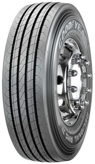
Figure 3.
Image depicting a 315/80R22.5 Goodyear RHS II Tire.
The tire’s sidewall and tread’s main material is rubber. Pneumatic tires consist of a rubber-like structure with different layers, including various rubber compounds, and are reinforced with steel-belted construction as rebar elements at the carcass and embedded steel wires in the beads filler. These are chosen due to their flexibility, high abrasion resistance, provision of good friction, and low hysteresis. The main physical structure of the tire consists of a carcass, a few layers of belts, beads, tread, and a tread base. The carcass acts as a shock absorber while supporting the vehicle’s load in various conditions. The belts consist of a rubber matrix and reinforced steel cords and are layered between the carcass and tread base. The carcass adds stiffness to the tread while restricting the deformation of the carcass piles and road-surface-impact irregularities. The tread is the main point of contact of the tire with the road and is made of solid rubber and carbon black for reinforcement and wear resistance. The tread protects the belt plies and carcass while providing the necessary frictional contact. The beads anchor the carcass plies and strengthen the tire rim assembly, preventing the rocking and slipping of the tire. The beads are made of hard-drawn steel wires to provide the desired rigidity and strength. The tire model consists of three-dimensional Mooney–Rivlin hyperelastic solid elements for the rubber material, two-dimensional fiber-reinforced layered membrane elements for the reinforced rubber composites, and one-dimensional beam elements for the two beads. The strain energy density function for the Mooney–Rivlin hyperelastic material, modified for non-vanishing compressibility, is:
where , , and are the three invariants of the right Cauchy–Green deformation tensor. The second Piola–Kirchhoff stress tensor follows from:
and the constitutive law tensor components follow from:
If B = 0, the material degenerates into the “Neo-Hookean” material. The term that adds compressibility, can be chosen in the form:
The coefficients A and B are material parameters, while coefficient C provides equilibrium at zero strain and depends on coefficients A and B, and coefficient D is a penalty factor that depends on the equivalent Poisson’s ratio, as shown below. If the material tends to be incompressible, then the value of = (relative volume)2 tends towards 1, and the penalty factor, D, tends towards infinity; in other words, the greater D is, the less compressible the material will be. Coefficient C depends on the coefficients A and B, as shown in Equation (6).
The material assumption for the computational simulation in the contact model of the mechanical components was mostly homogeneous and isotropic. In this work, the rubber parts are assumed to be homogeneous, isotropic, and hyperelastic and the material properties are shown in Table 1.

Table 1.
Solid elements material properties based on experimental testing.
In Pam-Crash finite element codes, the solid elements are implemented to carry out the discretization of the three-dimensional continuum media. The definition of the solid elements is presented based on trilinear shape functions for the interpolation of the coordinates. An iso-parametric formulation is used to ensure the automatic satisfaction of the mesh convergence and completeness criteria; therefore, the same shape functions are used to interpolate the coordinates and the displacements. Thus, the first-order elements or solid elements implemented are computationally effective and efficient [14].
For computational simulations that are carried out through explicit calculations, where the time step is governed by the stability conditions, resulting in small-size elements, solid elements are used to solve the convergence issues, particularly in a finite element analysis of the tires. Solid elements provide a reasonable computational cost for tire-rolling simulations.
The truck tire rim assembly model shown in Figure 4 consists of 27 material definitions.
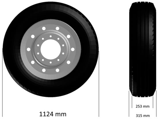
Figure 4.
RHS truck tire model dimensions.
A validation analysis was performed between the number of solid elements and the steady-state stage of the stress; finally, it was observed that the large number of elements (fine elements) for the rubbery parts resulted in an improvement in the accuracy after a certain mesh density with the selected hyperelastic material model in this work. Despite the coarse mesh for the tire sections, the finer mesh resulted in an easier convergence of the stress values to a stable value. Therefore, 3240 solid elements were chosen for the rubbery parts of the tire. The reinforcement layers of tires were modeled using 1800 membrane elements, 7316 thin shell elements, and 120 beam elements.
Most materials in tires exhibit a nonlinear stress–strain relationship under a wide range of loading conditions. The carcass and belts were modeled using elastic, three-layered membrane elements, consisting of two layers of cords controlled in two directions, and a single-layer isotropic matrix, with the radial-ply cords embedded in the carcass from one bead to the other. Three-dimensional elements resembling the tread, tread base, tread shoulders, and bead fillers were added, along with their hyperelastic rubber material. The rim was defined as a rigid body for the simplicity of the model, as the rim deformation was negligible. The rim was based on a conventional steel rim with a Young’s Modulus of 200 GPa.
2.1.2. Tire Model Validation
A static model validation comprises two tests—a footprint test and a vertical stiffness test. The footprint test shown in Figure 5 involved the application of a constant vertical load being applied to the tire to figure out the tire’s contact area. Vertical loads of 11.3, 22.5, and 45.0 kN were applied to the tire’s center on a hard flat surface, causing the tire to deform at its contact area. The total run time of the test was two seconds and the contact area was measured.

Figure 5.
Sample footprint test results at 427.5 kPa inflation pressure and 45 kN vertical load.
The results of the footprint test, consisting of the contact area at various inflation pressures and vertical loads, are shown in Figure 6. Based on the results, an increase in the inflation pressure resulted in a decrease in the contact area, whereas an increase in the vertical load resulted in an increase in the contact area in a non-linear fashion, and this trend was the same for all tire pressures. The data from the test were in agreement with the existing theory of inflation pressure and contact area. At an 11.3 kN vertical load, halving the pressure to 427.5 kPa reduced the contact area by 63%, whereas an increase of 50% in the pressure increased the contact area by 52%. At a 22.5 kN vertical load, halving the pressure to 427.5 kPa reduced the contact area by 37%, whereas an increase of 50% in the pressure increased the contact area by 92%. At a 45 kN vertical load, halving the pressure to 427.5 kPa reduced the contact area by 33%, whereas an increase of 50% in the pressure increased the contact area by 113%.
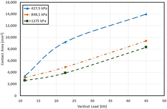
Figure 6.
Footprint FEA test graph at 427.5 kPa, 848.1 kPa, and 1275 kPa inflation pressure.
The vertical stiffness test was used to calculate the tire’s vertical stiffness, and was defined as below;
where this is called the spring rate and is performed over a hard surface. The center of the truck was contained in longitudinal, lateral translational, and all rotational directions. A quasi-static low-rate ramp loading was applied to the tire’s center, causing it to deform gradually, with the deformations at various vertical loads being recorded. The slope of the tire deflection vs. the load was calculated, with the obtained value considered to be the tire’s vertical stiffness. The table highlights the simulated and measured vertical stiffness values of the RHS tire at various inflation pressures. It should be noted that an inflation of 848.1 kPa was the only inflation pressure used for the physical test. The error between the simulated and measured vertical stiffnesses at 848.1 kPa was 0.97%, which revealed a good agreement with the manufacturer data provided. The vertical stiffness had a proportional and linear relationship with the inflation pressure, as an increase in the inflation pressure increased the tire’s vertical stiffness, as shown in Table 2. It should be noted that the vertical stiffness of the tire was only measured at the nominal inflation pressure of 848 kPa and that the vertical stiffness was also not a function of the applied vertical load.
Table 2.
Simulated and measured vertical stiffness data.
Dynamic validation consists of two tests—a cornering stiffness test and a drum-cleat test. The main purpose of a dynamic test is to observe the reaction of the tire in motion. A drum-cleat test is used to evaluate the horizontal and vertical vibration modes of an RHS tire. A 2.5 m diameter rigid drum with a 15 mm radius cleat was positioned below the tire, as shown in Figure 7, and the drum was subjected to an 11.1 rad/s angular velocity to excite the tire. The tire was locked in the vertical axis after 0.1 s of simulation time to avoid unnecessary bouncing movements during the excitation. Other parameters such as vertical loads were constant, whereas the inflation pressures were varied at the three inflation pressures used for the previous tests. This was performed because previous research has demonstrated that inflation pressure has the greatest influence on vibration modes [6]. The horizontal and vertical focus on the tire’s center were measured in the time domain and then converted to the frequency domain via the Fast Fourier Transform (FFT) algorithms implemented by previous researchers [6]. The first vertical and horizontal modes listed in Table 3 were estimated at a vertical load of 26.7 kN using the three testing inflation pressures. Increasing the inflation pressure increased the frequencies of the horizontal and vertical modes, which is consistent with previous research.
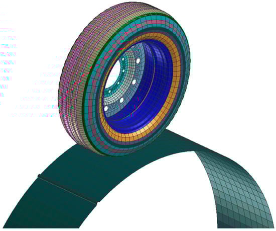
Figure 7.
Drum-cleat test overview.
Table 3.
Horizontal and vertical vibration modes.
The RHS tire was subjected to a dynamic cornering test to evaluate the tire’s cornering stiffness, as shown in Figure 8. The tire was first inflated to the three mentioned inflation pressures and the vertical load was applied to the tire’s center, with a longitudinal velocity also applied to the tire’s center. The simulation run time was 3 s and the tire was pre-steered to angles varying from 0 to 12 degrees, allowing for an examination of the effect of the cornering angle on the tire’s operational performance.
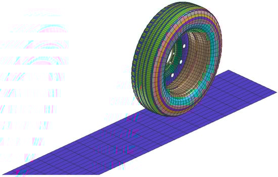
Figure 8.
RHS cornering test setup at 2-degree slip angle.
The cornering stiffness at 0 degrees was estimated by taking the slope of the lateral force curve between two data points at 0- and 2-degree steering angles. The experimental and simulated cornering stiffness values shown in Table 4 were in good agreement, with an error of only 1.68%.
Table 4.
Cornering stiffness comparison of experimental and simulated at nominal operating conditions.
2.2. Tire–Road Model Setup
The basic methodology of the contact mechanics in this simulation followed the Node to Surface contact as shown in Figure 9. For large deformation contact, node-to-surface contact elements were used [15]. The implemented contact method in this research was a penalty method, where penetration was allowed but not penalized [14]. The discretization of the variables is the only requirement for the standard penalty method. The penalty force can be calculated with three different solutions: linear penalty, non-linear penalty, and kinematic iterative [14].
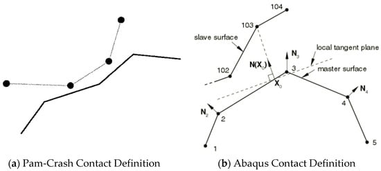
Figure 9.
Definition of the anchor point and local tangent plane used by the small-sliding, node-to-surface formulation for node 103 at Abaqus 6.14 (Reprinted/adapted with permission from Ref. [16]).
In the node-to-surface contact, the slave nodes should not penetrate the master segments; therefore, for the quality of the solution, a contact thickness of 5 mm and sliding interface penalties of 0.1 were defined for the tread elements at the contact patch and road. It should be noted that this treatment was not symmetric. To model the real tire–road interactions, a non-penetration node to the surface was defined to prevent the tire nodes from penetrating the road surface elements during the analysis. The surface length varied in distance to adequately cover the distance traveled by the tires during the two-second period.
To determine the tire–road contact interface, the frictional contact with Coulomb’s law was implemented. According to Coulomb’s law, sliding occurred once the tangential force was larger than a specific limit, as shown in Figure 10.
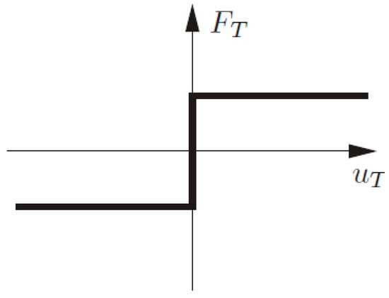
Figure 10.
Coulomb’s friction law.
The slave and master’s bodies no longer stick to each other after certain limits and this condition tangential force, , is called sliding, and can be described by Equation (8). In this sliding condition, the tire rolls relatively to the road in the Arbitrary Lagrangian-Eulerian (ALE) Framework.
where μ is the sliding friction coefficient [15]. To define a non-symmetric node to segment with edge treatment, for the rolling tire over the dry hard surface, a constant friction coefficient of 0.8 was considered in the Pam-Crash software. It should be mentioned that the tire rim setup was considered with no sliding and friction, and the internal temperature between the tire and terrain was ignored in this research.
Figure 11 shows the tire forces in the global and local coordinates used to derive the lateral force at the tire slip angle . The mathematics equation to compute the lateral force is defined as and is presented as Equation (9).
where is the tire longitudinal force or tire tractive force that is developed during braking and acceleration. The term is the tire’s lateral force component in the Y direction, which is generated as the tire is steered. It also has the capability of controlling the vehicle [2].
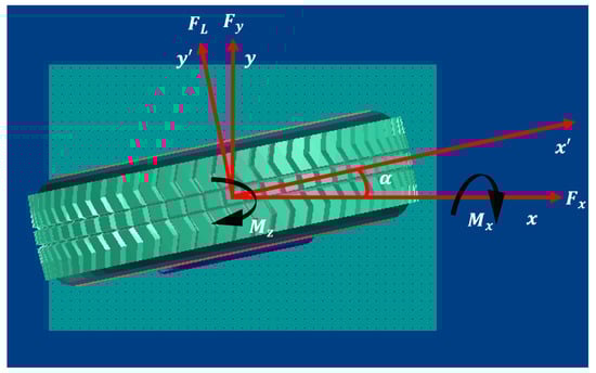
Figure 11.
Cornering forces and moments for a steered tire.
3. Tire–Road Interaction Results and Discussion
The simulation of an RHS 315/80R22.5 tire rolling on a dry, hard surface without any road unevenness was carried out under various operating conditions, including three different speeds, three various inflation pressures, and three different vertical loads, via an explicit solver in the Pam-Crash finite element software. The slip angle varied between 0 and 12 degrees. The three speeds used for this study were 10, 50, and 100 km/h, which were selected to cover the range of operating speeds for this specific tire type (the tire is rated for 80 km/h in EU and 100 km/h in the USA). In addition, three vertical loads and inflation pressures were used to model under, nominal, and over conditions. In addition, all the forces were extracted from the tire–road contact forces in the steady-state condition. Moreover, the moments, especially the self-aligning moment, were extracted from the tire section. Finally, the results are presented here for a better comparison.
3.1. Lateral Contact Force
To compare the tire behavior in different operating conditions, three various situations are presented here for the tire-cornering force at slip angles of 0–12 degrees.
According to Figure 12, the lateral force varied linearly at slip angles below the +4 degree (positive slip angles), which resulted in a linear relationship between the lateral force and slip angles at a constant inflation pressure and certain speed. Therefore, the cornering stiffness could be determined as a linear equation in the range between the 0- and 4-degree slip angles [2]. It must be noted that the lateral force was described as a linear approximation at small slip angles that were lower than 4 degrees [11]. Moreover, Figure 12 reveals that increasing the applied vertical load on the tire rim led to the generation of a higher lateral force. It can be seen that the lateral force was by far at its maximum value with the 53.4 kN vertical load. It rose dramatically to a peak of approximately 33 kN with the 53.4 kN load, which made the tire realign strongly into its initial or original position in the direction of the traveling, due to large inertia forces.
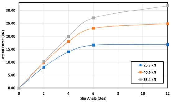
Figure 12.
Effect of slip angle and load on lateral force with 848.1 kPa inflation pressure and 100 km/h speed at 26.7 kN, 40.0 kN, and 53.4 kN vertical loads.
Furthermore, with the existence of higher vertical loads and larger slip angles, the compression of the tread blocks in the contact patch was much greater, regardless of the tire speed. Therefore, the tread blocks (the tread elements in both the tread and under-tread areas) generated a higher deflection in the lateral direction, which increased the deformation of the contact zone [17]. It can also be noted that an increase in the vertical load in the presence of a constant inflation pressure would directly increase the contact length of the tire–terrain interaction. However, the observed drop in the lateral force at larger slip angles may be the reason for the decrease in the lateral stiffness of the tire and increase in the longitudinal force. Additionally, the lateral force remained relatively stable, at between 6- and 12-degree slip angles with the 26.7 kN load, regardless of increases in the slip angles and cornering stiffness following a non-linear dominate in this range (after passing a 6-degree slip angle). On the other hand, it must be noted that an increase in the tire slip angle may also increase the frictional resistance at the rigid wheel/rim and tire while sliding occurs in the tire–terrain interaction [18], which would lead to the generation of a higher lateral force at a constant inflation pressure and vertical load.
Figure 13 presents the results of the changes in the lateral force with variations in the operating speeds. According to Figure 13, a higher longitudinal speed provided a lower lateral force at small slip angles and followed a linear increasing trend. Although at larger slip angles, lateral force is directly affected by speed, at lower slip angles (below 4 degrees), lateral force can be estimated as completely linear, and it followed an increasing constant path for all three speeds. However, a drop in the longitudinal velocity led to the generation of small movements of the wheel at larger slip angles; therefore, the tire would tend to generate a higher lateral force. Therefore, at greater slip angles (between 6 and 12 degrees), the lateral force was slightly increased to reach an approximately maximum value of 31 kN at 10 km/h. Moreover, at the 10 km/h speed, the deformation of the tire from the center line was considerably more than the tires traveling at the 50 km/h and 100 km/h speeds. At larger slip angles, the value of the speed did not have a significant effect on the lateral force, and it provided a negligible amount of lateral force at the 12-degree slip angles. However, it can be noted that, at larger slip angles, the tire produced a larger sliding zone due to a higher lateral force, which led to a decreased adhesive zone for the tread elements of the tire entering the tire–terrain contact zone [17]. Additionally, it can be inferred from Figure 13 that, at lower speeds (10 km/h and 50 km/h), the tread pattern of the tire may not have gripped the road completely, which resulted in the generation of a higher lateral force. Moreover, it can be mentioned that the lateral force saw only a small rise to approximately 25 kN with the 12-degree slip angles and the 100 km/h speed. In this way, the contact patch of the tire lost considerable friction with the ground, which was a dry, hard surface in this research.
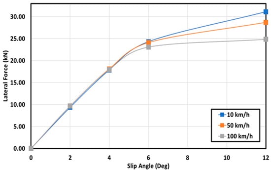
Figure 13.
Effect of slip angle and speed on lateral force with 1848.1 kPa inflation pressure and 53.4 kN load at 10 km/h, 50 km/h, and 100 km/h speed.
Figure 14 shows the variation in the lateral force as a function of the slip angle for the truck tire running at 100 km/h and different inflation pressures. The results from Figure 14 indicate that, at small slip angles and a higher inflation pressure, the tread elements deflected slightly and completely covered the contact zone; therefore, the sliding zone was much bigger with a linear cornering stiffness in the presence of a higher inflation pressure [19]. On the other hand, according to Figure 14, the lateral force was highly dependent on the tire inflation pressure and it could change remarkably due to the inflation pressure for a given speed. It was observed that, at a given speed and vertical load, an increase in the tire inflation pressure correlated to a decrease in the tire–terrain contact zone, which would directly lead to a reduction in the pneumatic trail. Therefore, both larger slip angles with a higher tire inflation pressure had a significant effect on the increase in the sliding of the rear contact zone of the tire–terrain contact patch, which resulted in a decrease in the tread adhesive zone [17].
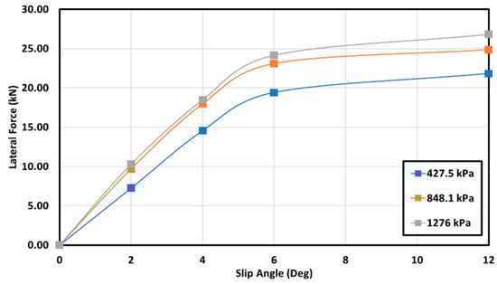
Figure 14.
Effect of slip angle and inflation pressure on lateral force with 100 km/h speed and 53.4 kN vertical load at 427.5 kPa, 848.1 kPa, and 1276 kPa inflation pressure.
In particular, the tire deflected laterally and was much stiffer at a higher inflation pressure with large slip angles (6–12 degrees). Additionally, by increasing the tire inflation pressure, the tire exhibited a higher cornering stiffness (slope of the lateral force versus slip angle 12 at zero slip angle), generating a higher lateral force, which resulted in an increased contact pressure. Consequently, the tire would tend to deflect strongly to develop a higher self-aligning moment [20]. On the contrary, the tire showed a high anti-skidding performance at a lower inflation pressure with small slip angles (below 4 degrees) [6].
3.2. Self-Aligning Moment
The tire self-aligning moment was extracted from the tire section under steady-state conditions in all the simulations. Additionally, to obtain parametric studies, the aligning moments were plotted versus the slip angles in the vertical axis, and the results are presented here.
It can be observed in Figure 15 that an increase in the vertical load on the tire resulted in a higher self-aligning moment for a given slip angle. This was expected due to the contact patch increase as the load increased, which led to a larger pneumatic trail; hence, for a set of given conditions, there would be an increase in the self-aligning moment. As the slip angle increased, an increase could be seen for the self-aligning moments up to 2–4 degrees. This was expected, as a similar trend could be seen for the lateral force relative to the slip angles, and the lateral force was directly proportional to the self-aligning moment. Above a 4-degree slip angle, the self-aligning moment could be seen to decrease, which corresponded to the lateral force saturating for the same range of cornering.
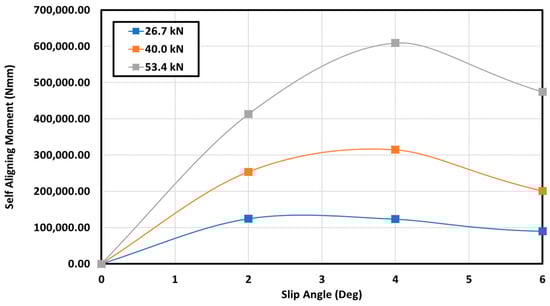
Figure 15.
Effect of slip angle on the self-aligning moment with 1276 kPa inflation pressure, and 100 km/h at 26.7 kN, 40.0 kN, and 53.4 kN.
In Figure 16, the variation in the self-aligning moment as a function of the slip angle for the RHS truck tire, running at a nominal inflation pressure of 848.1 kPa and several longitudinal speeds, is shown. It can be observed that the self-aligning moment for all the speed curves increased parabolically, approaching the 4-degree slip angle, and then declined at higher slip angles. The self-aligning moment can be seen to decrease with speed for a given slip angle. As the self-aligning moment had a relationship relative to the lateral force, a similar trend can be observed in Figure 13, where there was also a decrease in the lateral force as the speed increased for a given slip angle.
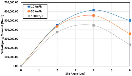
Figure 16.
Effect of slip angle on the self-aligning moment with 848.1 kPa inflation pressure, and 53.4 kN at 10 km/h, 50 km/h, and 100 km/h.
In Figure 17, the effect of the slip angle on the self-aligning moment at a 100 km/h longitudinal speed and several inflation pressures is shown. It can be seen that the self-aligning moment decreased with an increase in the inflation pressure at a given vertical load. This was expected, as an increase in inflation pressure would decrease the contact area of the tire and terrain, which would significantly reduce the pneumatic trail, resulting in a lower self-aligning moment for a given slip angle.
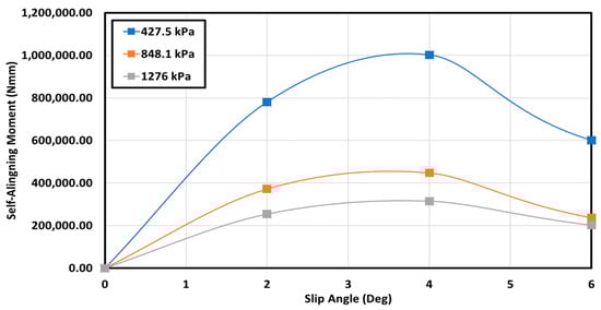
Figure 17.
Effect of slip angle on the self-aligning moment with 100 km/h longitudinal speed and 53.4 kN at 427.5 kPa, 848.1 kPa, and 1276 kPa.
4. Conclusions
A finite element model for a Regional Haul Steer II, RHS 315/80 R22.5 truck tire was developed using the Pam-Crash software. The truck tire rim assembly model consisted of 27 material definitions with 3240 solid elements, 1800 membrane elements, and 120 beam elements. The tire was then validated against physical measurements using static and dynamic domain tests, including the contact patch, vertical stiffness, first mode of vibration, and cornering stiffness tests. It was concluded that the modeled truck tire exhibited similar behavior to the actual test tire and could be used for further truck tire–road interaction analyses.
Furthermore, an investigation of the effects of several operating conditions on the tire-cornering characteristics over a hard surface was conducted. The operating conditions included three inflation pressures, three vertical loads, and three longitudinal speeds. It was found that the lateral force varied linearly at slip angles below +4 degrees (positive slip angles), which resulted in a linear relationship between the lateral force and slip angles at given inflation pressures and longitudinal speeds. Additionally, a higher longitudinal speed provided a lower lateral force at small slip angles, and it followed a linear increasing trend. Regarding the self-aligning moment, it could be seen to increase parabolically for all the speed curves, approaching the 4-degree slip angle, and then decline at higher slip angles.
This research will continue and expand to investigate the cornering characteristics of truck tires over flooded surfaces under different operating conditions.
Author Contributions
Conceptualization Z.E.-S. and M.E.-G.; Methodology H.F. and M.K.; validation H.F.; formal analysis H.F. and M.K.; investigation Z.E.-S. and H.F.; resources H.F., Data curation H.F. and M.K.; supervision Z.E.-S. and M.E.-G. All authors have read and agreed to the published version of the manuscript.
Funding
This research received no external funding.
Data Availability Statement
The data published in this journal paper are available upon request. Please email the corresponding author for details.
Acknowledgments
The authors would like to acknowledge Volvo Groups Trucks Technology and NSERC for support during this project.
Conflicts of Interest
The authors declare no conflict of interest.
References
- Loeb, J.S.; Guenther, D.A.; Chen, H.-H.F.; Ellis, J.R. Lateral stiffness, cornering stiffness and relaxation length of the pneumatic tire. SAE Trans. 1990, 99, 147–155. [Google Scholar]
- Wong, J.Y. Theory of Ground Vehicles; John Wiley & Sons: Hoboken, NJ, USA, 2022. [Google Scholar]
- Xia, X.; Xiong, L.; Lin, X.; Yu, Z. Vehicle Sideslip Angle Estimation Considering the Tire Pneumatic Trail Variation; 0148-7191 SAE Technical Paper; SAE: Warrendale, PA, USA, 2018. [Google Scholar]
- Heisler, H. Advanced Vehicle Technology; Elsevier: Amsterdam, The Netherlands, 2002. [Google Scholar]
- El-Sayegh, Z.; El-Gindy, M. Cornering characteristics of a truck tire on wet surface using finite element analysis and smoothed-particle hydrodynamics. Int. J. Dyn. Control. 2018, 6, 1567–1576. [Google Scholar] [CrossRef]
- Anupam, K.; Srirangam, S.; Scarpas, A.; Kasbergen, C.; Kane, M. Study of cornering maneuvers of a pneumatic tire on asphalt pavement surfaces using the finite element method. Transp. Res. Rec. 2014, 2457, 129–139. [Google Scholar] [CrossRef]
- Oertel, C.; Wei, Y. Tyre rolling kinematics and prediction of tyre forces and moments: Part I–theory and method. Veh. Syst. Dyn. 2012, 50, 1673–1687. [Google Scholar] [CrossRef]
- Korunović, N.; Trajanović, M.; Stojković, M.; Mišić, D.; Milovanović, J. Finite element analysis of a tire steady rolling on the drum and comparison with experiment. Stroj. Vestn. J. Mech. Eng. 2011, 57, 888–897. [Google Scholar] [CrossRef]
- Ghoreishy, M. Steady state rolling analysis of a radial tyre: Comparison with experimental results. Proc. Inst. Mech. Eng. Part D J. Automob. Eng. 2006, 220, 713–721. [Google Scholar] [CrossRef]
- Baffet, G.; Charara, A.; Stephant, J. Sideslip angle, lateral tire force and road friction estimation in simulations and experiments. In Proceedings of the 2006 IEEE Conference on Computer Aided Control System Design, 2006 IEEE International Conference on Control Applications, 2006 IEEE International Symposium on Intelligent Control, Munich, Germany, 4–6 October 2006; pp. 903–908. [Google Scholar]
- Tönük, E.; Ünlüsoy, Y.S. Prediction of automobile tire cornering force characteristics by finite element modeling and analysis. Comput. Struct. 2001, 79, 1219–1232. [Google Scholar] [CrossRef]
- Kabe, K.; Koishi, M. Tire cornering simulation using finite element analysis. J. Appl. Polym. Sci. 2000, 78, 1566–1572. [Google Scholar] [CrossRef]
- Dixon, J.C. Tires, Suspension and Handling; SAE International: Warrendale, PA, USA, 1996. [Google Scholar]
- Group, E. Pam-Crash Theory Notes Manual; Pam System International: Joliet, IL, USA, 2000. [Google Scholar]
- Wriggers, P.; Laursen, T.A. Computational Contact Mechanics; Springer: Berlin/Heidelberg, Germany, 2006; Volume 2. [Google Scholar]
- Simulia, D.S. ABAQUS Analysis User’s Manual (Version 6.14); Dassault Systèmes Simulia: Providence, RI, USA, 2016. [Google Scholar]
- Huang, H.-H.; Tsai, M.-J. Vehicle Cornering Performance Evaluation and Enhancement Based on CAE and Experimental Analyses. Appl. Sci. 2019, 9, 5428. [Google Scholar] [CrossRef]
- Ozaki, S.; Kondo, W. Finite element analysis of tire traveling performance using anisotropic frictional interaction model. J. Terra. 2016, 64, 1–9. [Google Scholar] [CrossRef]
- Sabey, B.E. Road surface characteristics and skidding resistance. Rubber Chem. Technol. 1967, 40, 684–693. [Google Scholar] [CrossRef]
- Reiter, M.; Wagner, J. Automated automotive tire inflation system–effect of tire pressure on vehicle handling. IFAC Proc. Vol. 2010, 43, 638–643. [Google Scholar] [CrossRef]
Disclaimer/Publisher’s Note: The statements, opinions and data contained in all publications are solely those of the individual author(s) and contributor(s) and not of MDPI and/or the editor(s). MDPI and/or the editor(s) disclaim responsibility for any injury to people or property resulting from any ideas, methods, instructions or products referred to in the content. |
© 2023 by the authors. Licensee MDPI, Basel, Switzerland. This article is an open access article distributed under the terms and conditions of the Creative Commons Attribution (CC BY) license (https://creativecommons.org/licenses/by/4.0/).