Finite-Time Super Twisting Disturbance Observer-Based Backstepping Control for Body-Flap Hypersonic Vehicle

Abstract

This paper investigates the attitude control problem for underactuated body-flap hypersonic vehicles (BFHSVs) with mixed disturbances. First, the control-oriented model for BFHSV is introduced. Then, an improved finite-time super twisting disturbance observer (STDO) is designed. Finite-time convergence of estimate error and smoother inputs are achieved. Meanwhile, a parametric command method is introduced to calculate the differential of inputs which can enhance the dynamic response of the closed-loop system. Subsequently, the virtual control signal is derived by a second-order filter to avoid the differential explosion problem. The overall stability of the closed-loop system is demonstrated by applying the Lyapunov stability theory. Finally, the performance of the proposed control scheme is evaluated through extensive and comparative numerical simulations under multiple disturbances.

1. Introduction

Hypersonic vehicles (HSVs) have attracted increasing attention due to their unique features of both an aircraft and a spacecraft. Due to their wide speed range and large flight envelope, they need to have a high lift-to-drag ratio and good thermal protection capabilities, and the traditional aerodynamic shape of the aircraft is no longer applicable. From the reusable launch vehicle to the X-37B, the shape of the large-lift body has gradually become the main aerodynamic shape for the HSV [1]. Among them, the body-flap hypersonic vehicle (BFHSV) such as HTV-2 with combined wave-rider and lifting-body has been developed. The whole fuselage has only two flaps, which not only reduce weight and energy consumption but also further improve the lift-to-drag ratio, effectively avoiding aerodynamic heating and thermal protection issues. This trend is expected to continue in future development [2]

In recent years, nonlinear control methods have replaced linear control methods for the attitude control of HSVs. The backstepping method has shown excellent ability in dealing with the complex dynamics of hypersonic vehicles [3,4,5]. Sliding mode control has strong robustness to model uncertainties [6], and many better control methods have been derived [7,8,9]. Additionally, methods such as fuzzy control [10] and intelligent control [11,12,13], which are independent of specific model knowledge, have also been developed for hypersonic vehicles. However, all the above approaches are based on the theory that hypersonic vehicles can provide three-axis moments. For a body-flap hypersonic vehicle, the number of actuators in the system is less than the number of degrees of freedom to be controlled, resulting in an underactuated system. The underactuated system does not have a complete relative order and is a nonminimum phase system. The system is transformed into a cascaded form of a linear system and a nonlinear system after feedback linearization. The linear part is the external dynamics and the relevant state is called the external state; the nonlinear part is the internal dynamics, and the corresponding state is called the internal state [14]. Neglecting the stability of the internal dynamics and directly applying these methods to the system can result in unexpected oscillations or even loss of stability of the overall system, which will cause server flight accidents. A study [15] used phase diagrams to judge the internal dynamic stability within underactuated systems, proposed the concept of optimal bounded inverse, converted the internal dynamic stability problem into a trajectory optimization problem, and designed an anti-windup backstepping controller. Another study [16] proposed a criterion for determining the stability of internal dynamics, pointing out that the stability of the internal dynamics of this type of vehicle is related to its lateral control departure parameter (LCDP) [17], linking control stability and aerodynamic characteristics. However, both of them only studied the control problem with instable internal dynamics, and it is essential to study the BFHSV stability control of the internal dynamic which is stable.

Another realistic problem is disturbance and uncertainty. Due to its excellent performance in anti-disturbance and convergence time, sliding mode control (SMC) is a popular choice for designing controllers of nonlinear systems [18,19,20,21]. In a study [22], SMC combined with learning controllers was designed for a T-S fuzzy system of HSVs, and a sliding mode-based extended state observer (ESO) was employed to estimate unmodeled dynamics. Another study [23] combines adaptive techniques to alleviate the chattering in sliding mode-based backstepping control for the HSV. Ju et al. [24] designed a fractional-order SMC, which allows the unsaturated state of the reusable launch vehicle to be executed to a predetermined residual at the origin and within a fixed time interval. A novel multivariable robust adaptive SMC scheme is designed in [25] based on super twisting algorithms to surmount the uncertainties from the unmodeled dynamics and the lumped disturbances. A study [26] designed a disturbance observer and a controller using terminal sliding mode and super twisting approaches, respectively, for the nonlinear systems of HSVs. The essence of SMC is to use the switching function to control the state to a suitable sliding mode surface, but the existence of switching items will lead to chattering problems. To date, few works of literature have considered both the finite-time stability and output chattering problems of SMC, which is still challenging for practical applications.

Inspired by the discussions above, the purpose of this paper is to present a control method for BFHSVs that can achieve accurate command tracking from the guidance system. This paper focuses on attitude control for the body-flap hypersonic vehicle. The main contributions include:

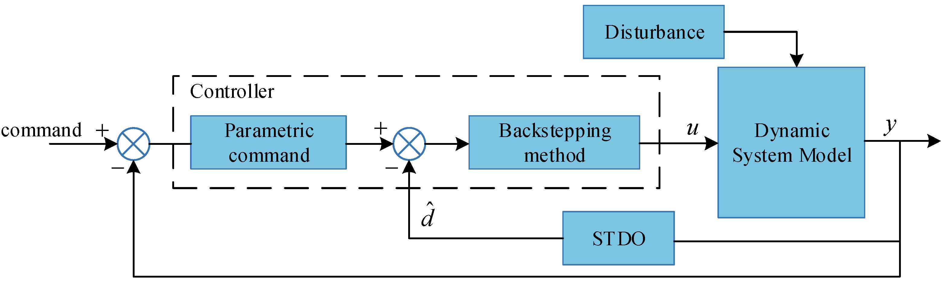
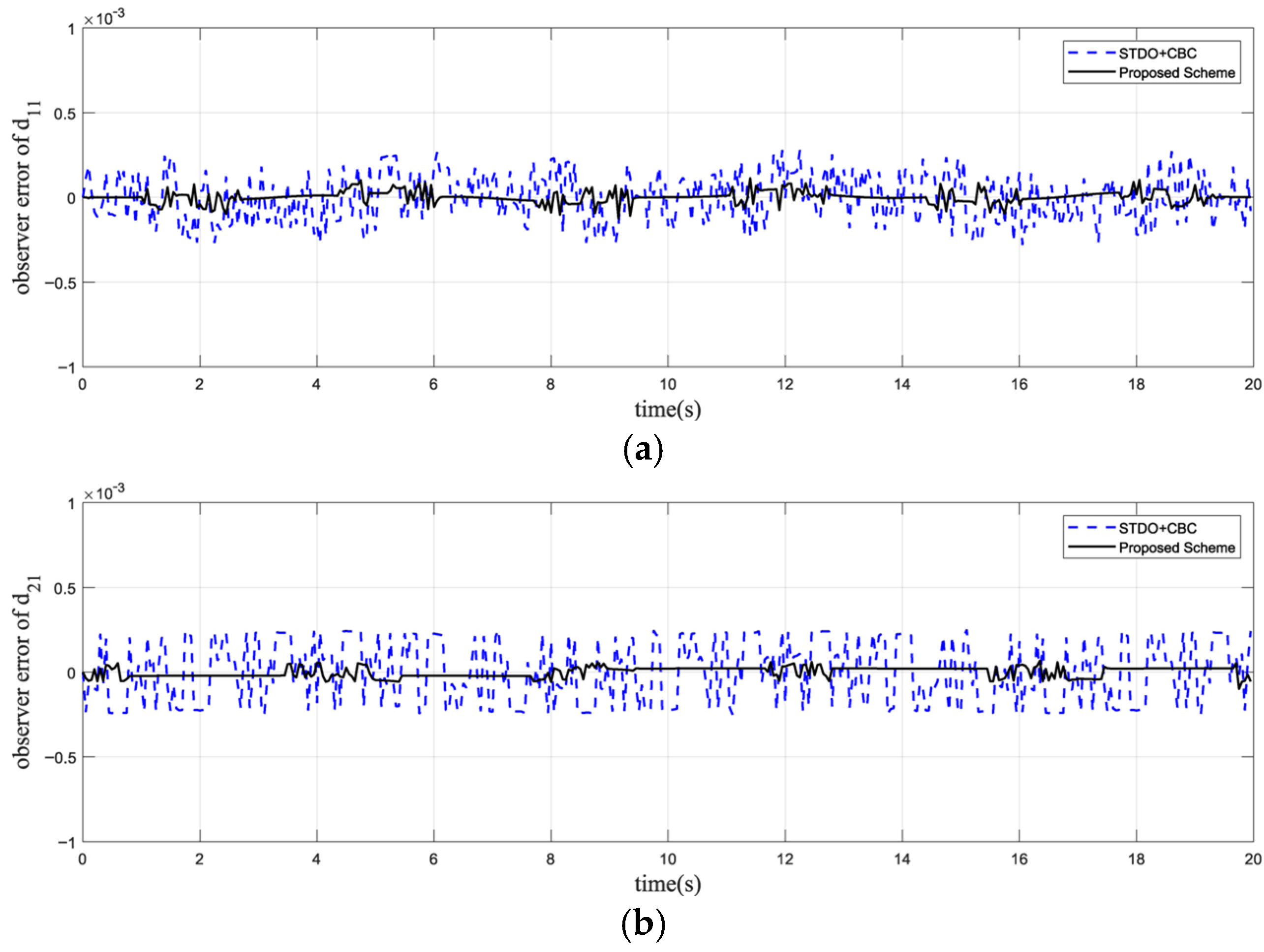
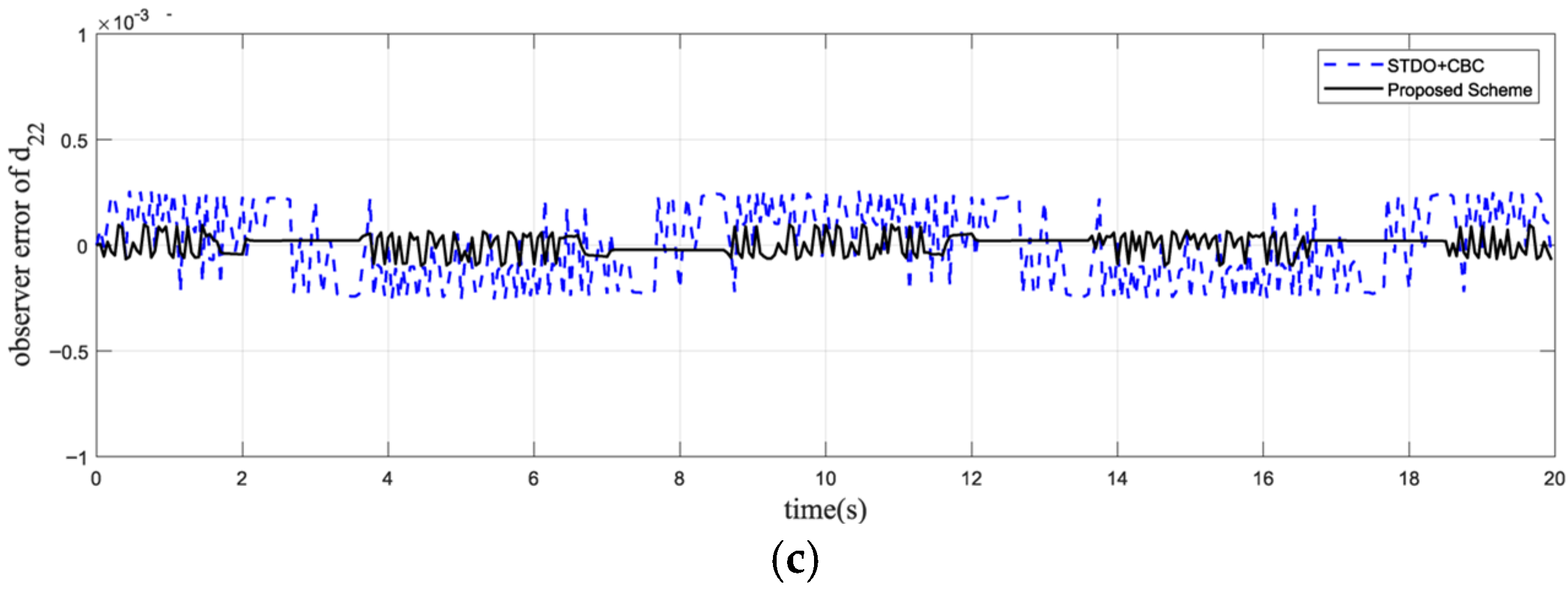
• The proposed STDO is employed for the lumped disturbances of a BFHSV, which has a smaller estimation error and smoother control variables than conventional super twisting approaches.
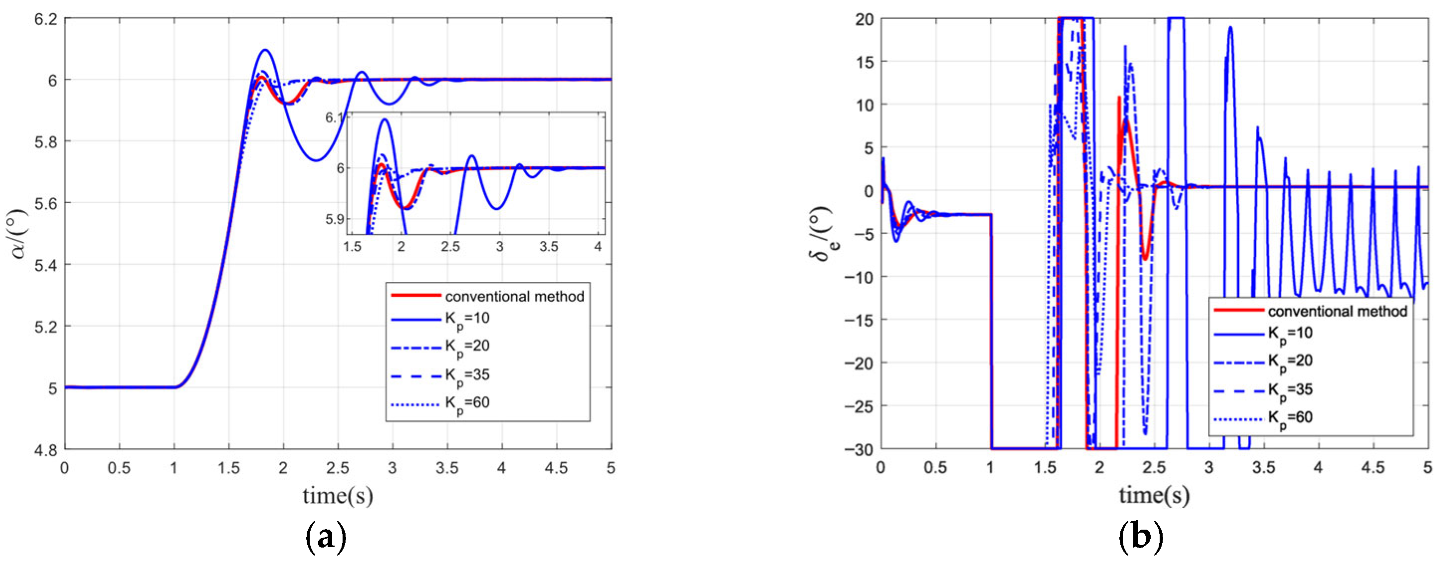
• The parametric command method can strengthen the states’ convergence speed of the backstepping control method. In addition, the “explosion of complexity” is avoided by introducing a second-order filter.

The remainder of this paper is organized as follows. Section 2 introduces the strict feedback model of the BFHSV. In Section 3, the STDO is developed for the BFHSV system with its stability analysis. In Section 4, a robust backstepping controller is designed based on STDO, and the stability of the composite method is also analyzed. Section 5 presents the simulation results and analysis, followed by a conclusion to end the paper.

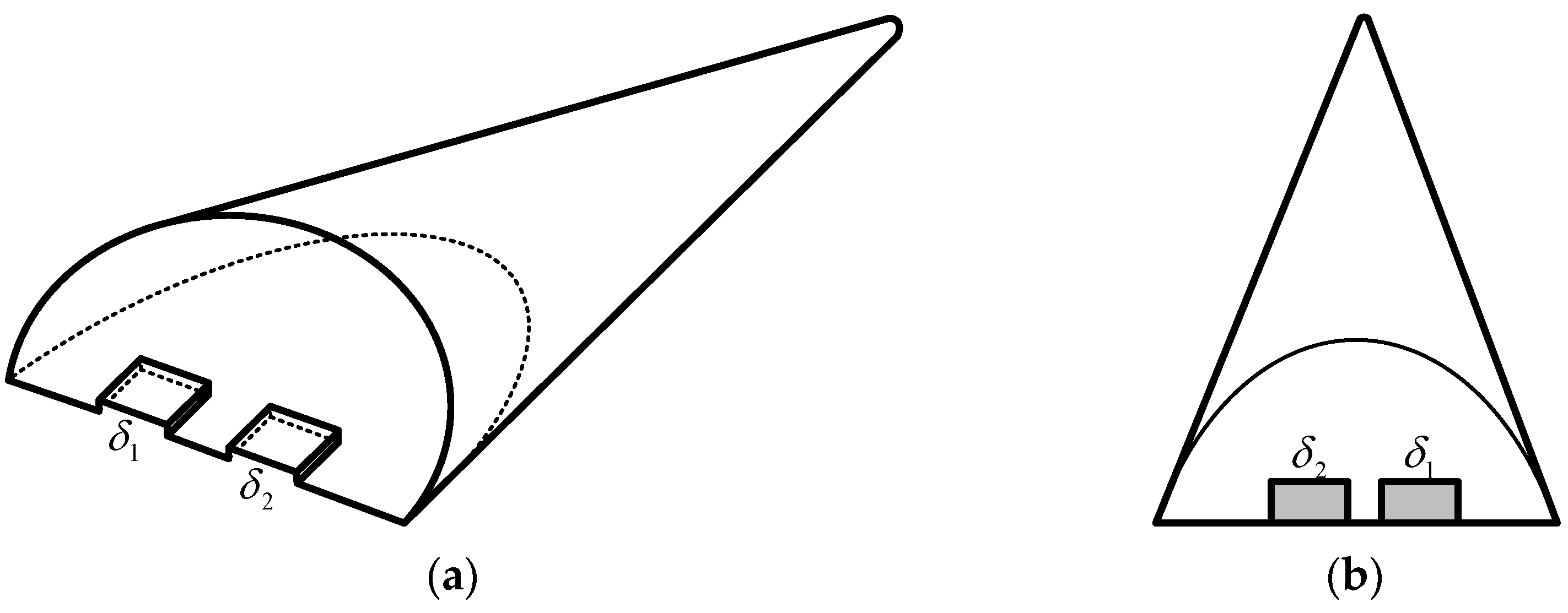
2. Problem Formulation

The attitude dynamics of a BFHSV are given as those of the HTV-2 model. As shown in Figure 1, the vehicle adopts a lifting-body configuration with two body flaps. However, it has several RCS thrusters which are used in low dynamic pressure regions. At the end of the cruise phase and the beginning of the dive phase, only two body flaps are available.

Both body flaps deflect in the same direction to act as an elevator and differentially deflect to act as an aileron, so the control variables ${\delta }_e$ and ${\delta }_a$ are defined as follows:

$$\begin{array}{l}{\delta }_e\triangleq \left({\delta }_1+{\delta }_2\right)/2\\ {\delta }_a\triangleq \left({\delta }_2-{\delta }_1\right)/2\end{array}$$

(1)

where, ${\delta }_1$ and ${\delta }_2$ are the left and right flaps, respectively.

The attitude dynamics of the BFHSV are written as follows:

$$\{\begin{array}{l}\dot{\alpha }={\omega }_z+{\omega }_y\sin \alpha \tan \beta -{\omega }_x\cos \alpha \tan \beta -\frac{Y}{mV\cos \beta }+\frac{g\cos \theta \cos {\gamma }_v}{V\cos \beta }\\ \dot{\beta }={\omega }_y\cos \alpha +{\omega }_x\sin \alpha +\frac{Z}{mV}+\frac{g\cos \theta \sin {\gamma }_v}{V}\\ {\dot{\gamma }}_v=\frac{{\omega }_x\cos \alpha -{\omega }_y\sin \alpha }{\cos \beta }+\frac{Y(\tan \theta \sin {\gamma }_v+\tan \beta )+Z\tan \theta \cos {\gamma }_v-mg\cos \theta \tan \beta \cos {\gamma }_v}{mV}\\ {\dot{\omega }}_x=-\frac{J_{xy}\left(J_x+J_y-J_z\right)}{J_x{J}_y-J_{xy}^2}{\omega }_x{\omega }_z+\frac{J_{xy}^2-J_y\left(J_z-J_y\right)}{J_x{J}_y-J_{xy}^2}{\omega }_y{\omega }_z+P_{\beta }^{\prime }\beta +P_{{\delta }_a}^{\prime }{\delta }_a\\ {\dot{\omega }}_y=-\frac{J_{xy}^2+J_x^2-J_x{J}_z}{J_x{J}_y-J_{xy}^2}{\omega }_x{\omega }_z+\frac{J_{xy}\left(J_x+J_y-J_z\right)}{J_x{J}_y-J_{xy}^2}{\omega }_y{\omega }_z+R_{\beta }^{\prime }\beta +R_{{\delta }_a}^{\prime }{\delta }_a\\ {\dot{\omega }}_z=\frac{J_x-J_y}{J_z}{\omega }_x{\omega }_y+\frac{J_{xy}}{J_z}\left({\omega }_x{}^2-{\omega }_y{}^2\right)+Q_{\alpha }^{\prime }\alpha +Q_{{\delta }_e}^{\prime }{\delta }_e\end{array}$$

(2)

where

$$\begin{array}{c}{P}_{\beta }^{\prime }=\frac{J_y{P}_{\beta }+J_{xy}{R}_{\beta }}{J_x{J}_y-J_{xy}^2}, P_{{\delta }_a}^{\prime }=\frac{J_y{P}_{{\delta }_a}+J_{xy}{R}_{{\delta }_a}}{J_x{J}_y-J_{xy}^2},\hfill \\ R_{\beta }^{\prime }=\frac{J_x{R}_{\beta }+J_{xy}{P}_{\beta }}{J_x{J}_y-J_{xy}^2}, R_{{\delta }_a}^{\prime }=\frac{J_x{R}_{{\delta }_a}+J_{xy}{P}_{{\delta }_a}}{J_x{J}_y-J_{xy}^2},\hfill \\ Q_{\alpha }^{\prime }=\frac{Q_{\alpha }}{J_z},\hspace{1em}\hspace{1em}\hspace{1em}{Q}_{{\delta }_e}^{\prime }=\frac{Q_{{\delta }_e}}{J_z}.\hfill \end{array}$$

In Model (2), state variables $\alpha$, $\beta$, ${\gamma }_v$, ${\omega }_x$, ${\omega }_y$, and ${\omega }_z$ denote the angle of attack, sideslip angle, bank angle, roll rate, yaw rate, and pitch rate, respectively. $J_x$, $J_y$, and $J_z$ represent the moments of inertia of the three body axes and $J_{xy}$ is the product of inertia. $V$, $m$, $\theta$, $Y$, and $Z$ are the velocity, mass, flight path angle, and lift and side forces of the vehicle, respectively. The notions $R_{\beta }^{\prime }$, $P_{\beta }^{\prime }$, $Q_{\alpha }^{\prime }$, $Q_{{\delta }_e}^{\prime }$, $R_{{\delta }_a}^{\prime }$, and $P_{{\delta }_a}^{\prime }$ denote the linearization of the contribution of sideslip to yaw and rolling moment, angle of attack and elevator to pitching moment, and aileron to yaw and rolling moment, respectively [27].

According to [28], the internal dynamics of a vehicle can stabilize if $LCDP<0$, and therefore the model of the BFHSV can be simplified to a parameter-strict feedback form as shown in Equation (3).

$$\begin{array}{l}{\dot{x}}_1=F_1+G_1{x}_2+d_1\\ {\dot{x}}_2=F_2+G_{2}u+d_2\end{array}$$

(3)

where $x_1={\left[\begin{array}{cc}\alpha & {\gamma }_v\end{array}\right]}^{{\rm T}}$, $x_2={\left[\begin{array}{cc}{\omega }_x& {\omega }_z\end{array}\right]}^{{\rm T}}$, $u={\left[\begin{array}{cc}{\delta }_e& {\delta }_a\end{array}\right]}^{{\rm T}}$, $d_1$, $d_2$ are equivalent disturbances caused by environment and model uncertainties and $F_1$, $F_2$, $G_1$, $G_2$ are defined as follows:

$$F_1=\left[\begin{array}{c}{\omega }_y\sin \alpha \tan \beta -\frac{Y}{mV\cos \beta }+\frac{g\cos \theta \cos {\gamma }_v}{V\cos \beta }\\ -\frac{{\omega }_y\sin \alpha }{\cos \beta }+\frac{Y(\tan \theta \sin {\gamma }_v+\tan \beta )+Z\tan \theta \cos {\gamma }_v-mg\cos \theta \tan \beta \cos {\gamma }_v}{mV}\end{array}\right]$$

(4)

$$F_2=\left[\begin{array}{c}-\frac{J_{xy}\left(J_x+J_y-J_z\right)}{J_x{J}_y-J_{xy}^2}{\omega }_x{\omega }_z+\frac{J_{xy}^2-J_y\left(J_z-J_y\right)}{J_x{J}_y-J_{xy}^2}{\omega }_y{\omega }_z+L_{\beta }^{\prime }\beta \\ \frac{J_x-J_y}{J_z}{\omega }_x{\omega }_y+\frac{J_{xy}}{J_z}\left({\omega }_x{}^2-{\omega }_y{}^2\right)+M_{\alpha }^{\prime }\alpha \end{array}\right]$$

(5)

$$G_1=\left[\begin{array}{cc}-\cos \alpha \tan \beta & 1\\ \frac{\cos \alpha }{\cos \beta }& 0\end{array}\right]$$

(6)

$$G_2=\left[\begin{array}{cc}0& {L^{\prime }}_{{\delta }_a}\\ {M^{\prime }}_{{\delta }_e}& 0\end{array}\right]$$

(7)

3. Super Twisting Algorithm Disturbance Observer Design

3.1. Observer Design

It can be seen that disturbances $d_i$ are independent of the differential equations without couplings. Thus, the observer for $d_i$ can be designed independently.

Assumption 1.

The disturbances $d_i$, $i=1,2$ are bounded, meaning that $\left|d_i\right|\le D_i, \left|{\dot{d}}_i\right|\le {\delta }_i$, where $D_i$ and ${\delta }_i$ are positive constants.

Inspired by the work in [29], an improved super twisting algorithm disturbance observer is developed to estimate the equivalent disturbance in finite time. The relevant auxiliary variables of the disturbance observer can be constructed as

$$\begin{array}{l}{\dot{z}}_1=F_1+G_1{x}_2+{\widehat{d}}_1\\ {\dot{z}}_2=F_2+G_2{u}_2+{\widehat{d}}_2\end{array}$$

(8)

The auxiliary sliding mode variables can be defined as

$$s_i=x_i-z_i$$

(9)

Thus, an observer for $d_i$ can be designed as

$${\widehat{d}}_i=k_{1i}{\lfloor s_i\rceil }^{{\mu }_{1i}}+k_{2i}{\displaystyle {\int }_0^t{\lfloor s_i\rceil }^{{\mu }_{2i}}d\tau }$$

(10)

where $k_{1i}$, $k_{2i}$, ${\mu }_{1i}\in \left(\frac{1}{2},1\right)$ and ${\mu }_{2i}=2{\mu }_{1i}-1$ are the parameters of the observer.

Notation 1.

For all $s={[s_1,s_2,\cdot \cdot \cdot s_n]}^T\in R^{n\times 1}$, the symbol ${\lfloor s\rceil }^q$ denotes ${\left[{\left|s_1\right|}^{q}sign(s_1),\cdot \cdot \cdot ,{\left|s_n\right|}^{q}sign(s_n)\right]}^T$.

3.2. Stability Analysis

Theorem 1.

With assumption 1 and the proposed disturbance observer (10), observation errors of $x_i$, $i=1, 2$ can converge in finite time to an arbitrarily small neighborhood of zero [30].

Proof of Theorem 1.

Recalling (9), it is not difficult to obtain that

$${\dot{s}}_i=d_i-{\widehat{d}}_i$$

(11)

Substituting Equation (10) into Equation (11) yields

$${\dot{s}}_i=d_i-k_{i1}{\lfloor s_i\rceil }^{{\mu }_{1i}}-k_{i2}{\displaystyle {\int }_0^t{\lfloor s_i\rceil }^{{\mu }_{2i}}d\tau }$$

(12)

In order to simplify the following derivation, we define ${\upsilon }_i=-k_{2i}{\displaystyle {\int }_0^t{\lfloor s_i\rceil }^{{\mu }_{2i}}d\tau }+d_i$. Then, Equation (12) can yield the following second-order system.

$$\{\begin{array}{c}{\dot{s}}_i=-k_{1i}{\lfloor s_i\rceil }^{{\mu }_{1i}}+{\upsilon }_i\\ {\dot{\upsilon }}_i=-k_{2i}{\lfloor s_i\rceil }^{{\mu }_{2i}}+d_i\end{array}$$

(13)

Due to the dependence on different channels in the error dynamic system Equation (13), all we need to demonstrate is that system Equation (14) possesses stable characteristics within a finite amount of time.

$$\{\begin{array}{c}\dot{s}=-k_1{\lfloor s\rceil }^{{\mu }_1}+\upsilon \\ \dot{\upsilon }=-k_2{\lfloor s\rceil }^{{\mu }_2}+d\end{array}$$

(14)

Consider the candidate Lyapunov function

$$V={\zeta }^{{\rm T}}Q\zeta$$

(15)

where $\zeta ={[{\lfloor s\rceil }^{{\mu }_1}, \upsilon ]}^{{\rm T}}$, $Q=\frac{1}{2{\mu }_1}\left[\begin{array}{cc}2k_2+{\mu }_1{k}_1^2& -{\mu }_1{k}_1\\ -{\mu }_1{k}_1& 2{\mu }_1\end{array}\right]$.

Notice that the Lyapunov function is continuously differentiable, except for the set $\mathsf{\Omega }=\{(s,\upsilon )|s=0\}$, and it can be acquired that

$${\lambda }_{\min }(Q){\Vert \zeta \Vert }^2\le V\le {\lambda }_{\max }(Q){\Vert \zeta \Vert }^2$$

(16)

where ${\lambda }_{\min }(\cdot )$ and ${\lambda }_{\max }(\cdot )$ are the minimum and maximum eigenvalues of the matrix $Q$.

By taking the derivative of both sides of Equation (15), we obtain:

$$\begin{array}{cc}\dot{V}\hfill & =\frac{1}{{\mu }_1}[{\lfloor s\rceil }^{{\mu }_1}, \upsilon ]\left[\begin{array}{cc}2k_2+{\mu }_1{k}_1^2& -{\mu }_1{k}_1\\ -{\mu }_1{k}_1& 2{\mu }_1\end{array}\right]\left[\begin{array}{c}{\mu }_1{\left|s\right|}^{{\mu }_1-1}(-k_1{\lfloor s\rceil }^{{\mu }_1}+\upsilon \\ \hfill -k_2{s}^{{\mu }_2}+d\hfill \end{array}\right]\hfill \\ & \le -{\left|s\right|}^{{\mu }_1-1}[(2k_2+{\mu }_1{k}_1^2)k_1{\left|s\right|}^{2{\mu }_1}+{\mu }_1{k}_1{\upsilon }^2-2k_1^2{\mu }_1{\lfloor s\rceil }^{{\mu }_1}\upsilon ]+{\zeta }^T\left[\begin{array}{c}{k}_1\\ -2\end{array}\right]d\\ & \le -{\left|s\right|}^{{\mu }_1-1}{\zeta }^{T}R\zeta +d\Vert \zeta \Vert \Vert h\Vert \hfill \end{array}$$

(17)

where $R=k_1\left[\begin{array}{cc}2k_2+{\mu }_1{k}_1^2& -{\mu }_1{k}_1\\ -{\mu }_1{k}_1& 2{\mu }_1\end{array}\right]$ and $h=\left[\begin{array}{c}{k}_1\\ -2\end{array}\right]$. From the definition of $\zeta$, we can obtain that:

$$R=k_1\left[\begin{array}{cc}2k_2+{\mu }_1{k}_1^2& -{\mu }_1{k}_1\\ -{\mu }_1{k}_1& 2{\mu }_1\end{array}\right]$$

(18)

Substituting (18) into (17) yields:

$$\begin{array}{cc}\dot{V}\hfill & \le -{\left|s\right|}^{{\mu }_1-1}{\lambda }_{\min }(R){\Vert \zeta \Vert }^2+d\Vert \zeta \Vert \Vert h\Vert \hfill \\ & \le -{\lambda }_{\min }(R){\Vert \zeta \Vert }^{(({\mu }_1+{\mu }_2)/{\mu }_1)}+d\Vert h\Vert {\lambda }_{\min }{(Q)}^{-(1/2)}{V}^{1/2}\hfill \\ & \le -{\lambda }_{\min }(R){\lambda }_{\min }{(Q)}^{-(({\mu }_{{}_1}+{\mu }_2)/2{\mu }_1)}{V}^{(({\mu }_{{}_1}+{\mu }_2)/2{\mu }_1)}+d\Vert h\Vert {\lambda }_{\min }{(Q)}^{-(1/2)}{V}^{1/2}\hfill \\ & \le -M_1{V}^{({\mu }_{{}_1}+{\mu }_2)/2{\mu }_1)}+M_2{V}^{1/2}\hfill \end{array}$$

(19)

where $M_1={\lambda }_{\min }(R){\lambda }_{\min }{(Q)}^{-(({\mu }_{{}_1}+{\mu }_2)/2{\mu }_1)}$, $M_2=d\Vert h\Vert {\lambda }_{\min }{(Q)}^{-(1/2)}$.

Recalling the setting rules of the STDO in Equation (12), ${\mu }_1\in (\frac{1}{2},1)$ and ${\mu }_2=2{\mu }_1-1$, we can obtain $\frac{{\mu }_1+{\mu }_2}{2{\mu }_1}\in (\frac{1}{2},1)$. According to [31], the system (14) is ultimately bounded in finite time, meaning that the variables $s$ and $\upsilon$ can stabilize to the origin $D_0$ within finite time $T_0$, and $D_0$ and $T_0$ can be expressed as

$$\begin{array}{c}{D}_0=\left\{\zeta |V(\zeta )<{\left(\frac{M_2}{\theta }\right)}^{2{\mu }_1/{\mu }_2}\right\},\theta \in \left(0,M_1\right)\hfill \\ T_0\le \frac{V{\left({\zeta }_0\right)}^{1-\frac{{\mu }_1+{\mu }_2}{2{\mu }_1}}}{\left(M_1-\theta \right)\left(1-\frac{{\mu }_1+{\mu }_2}{2{\mu }_1}\right)}\hfill \end{array}$$

(20)

That is, the equivalent disturbances $d_i$ can be estimated in finite time, and the corresponding max value of the convergence time can also be estimated. The proof of the STDO’s stability is complete. □

4. STDO-Based Improved Backstepping Controller Design

4.1. Improved Backstepping Controller Design

For the attitude system of a BFHSV, the desired command is $y_c={\left[a_c, {\gamma }_{v_c}\right]}^{{\rm T}}$. The attitude angle tracking error $e_1$ can be defined as $e_1=y_c-x_1$, whose differentiation is

$${\dot{e}}_1={\dot{y}}_c-F_1-G_1{x}_2-d_1$$

(21)

Considering $x_2$ as a virtual control variable, the desired virtual command can be defined as follows:

$$x_{2c}=G_1^{-1}(-F_1+{\dot{y}}_c+k_1{e}_1-{\widehat{d}}_1)$$

(22)

where $k_1$ is the designed positive definite diagonal matrix, ${\widehat{d}}_1$ is the estimate of the lumped disturbance by the STDO.

Virtual control Equation (22) needs to use the differential ${\dot{y}}_c$ of the attitude angle command. In the previous backstepping controller design work, the differential of the attitude angle command is obtained by deriving the command with respect to time as follows:

$${\dot{y}}_c={\left[\begin{array}{cc}\frac{{\alpha }_c}{\Delta t}& \frac{{\gamma }_{v_c}}{\Delta t}\end{array}\right]}^{{\rm T}}$$

(23)

where $\Delta t$ is the step size of the simulation.

In fact, there will be a situation where the rate of change of command conflicts with the command when the actual value of the attitude angle differs greatly from its desired value. For example, if the pitch channel is a step command of $5^{\circ }$ while the actual angle of attack is $0^{\circ }$, then the desired rate of change ${\dot{\alpha }}_c=0^{\circ }/s$. However, the system should have a large rate of change. It is contradictory to ${\dot{\alpha }}_c=0^{\circ }/s$, and the greater the gap between the desired value and the actual value, the more significant the contradiction will be. The method of directly deriving the attitude angle command only uses the desired value and does not consider the actual value. This method is only applicable when the tracking gap is small. When the tracking gap is larger, the control performance will be significantly worse.

As an improvement, the command of attitude angle change rate in this paper is as follows:

$${\dot{y}}_c={\left[\begin{array}{cc}\frac{{\alpha }_c-\alpha }{\Delta t}& \frac{{\gamma }_{v_c}-{\gamma }_v}{\Delta t}\end{array}\right]}^{{\rm T}}$$

(24)

Considering the actual dynamic characteristics of the control system itself, such as delay and overshoot, the corresponding process of the command cannot be completed within one control step. Therefore, the formula is modified appropriately, and a parametric calculation method for the change rate of the attitude angle command is proposed, that is,

$${\dot{y}}_c={\left[\begin{array}{cc}\frac{{\alpha }_c-\alpha }{K_p\Delta t}& \frac{{\gamma }_{v_c}-{\gamma }_v}{K_r\Delta t}\end{array}\right]}^{{\rm T}}$$

(25)

where $K_p$ and $K_r$ are the calculation parameters of the pitch and roll channels, respectively.

Remark 3.

An intuitional interpretation of Equation (25) is the desired value of the rate of change of attitude angle while Equation (23) is the change rate of the desired value. The actual value of the system is introduced into the parametric calculation method of change rate to improve the information utilization rate. It is not only suitable for the case of small tracking errors but also can realize fast and smooth tracking control under the condition of large tracking errors well. The response capability of the backstepping control system can be effectively adjusted by adjusting the calculation parameters.

Define $e_2=x_{2c}-x_2$ as the tracking error of the angular rate. Substituting Equation (22) into Equation (21) results in

$${\dot{e}}_1=-k_1{e}_1+G_1{e}_2+{\widehat{d}}_1-d_1$$

(26)

The angular rate error dynamics can be obtained as

$${\dot{e}}_2={\dot{x}}_{2c}-F_2-G_{2}u-d_2$$

(27)

Then, the control input variables are designed as follows:

$$u=G_2^{-1}(-F_2+{\dot{x}}_{2c}+G_1{e}_1+k_2{e}_2-{\widehat{d}}_2)$$

(28)

where $k_2$ is the designed positive definite diagonal matrix, ${\widehat{d}}_2$ is the estimate of the equivalent disturbance by the STDO.

Equations (27) and (28) contain the differentiation of the virtual control ${\dot{x}}_{2c}$, but it can be known from Equation (3) that the existence of uncertainty and nonlinearity makes the differentiation of the virtual input variable very difficult, and it may cause the “explosion of terms” problem. To solve this problem, a second-order filter proposed by Li et al. [32] is employed to estimate the differentiation of ${\dot{x}}_{2c}$, that is,

$${\dot{\overline{x}}}_{2c}=-\frac{{\overline{x}}_{2c}-x_{2c}}{{\tau }_1}-\frac{{\zeta }_{f1}({\overline{x}}_{2c}-x_{2c})}{\Vert {\overline{x}}_{2c}-x_{2c}\Vert +{\epsilon }_{f1}}$$

(29)

$${\widehat{x}}_{2c}=-\frac{{\widehat{x}}_{2c}-{\dot{\overline{x}}}_{2c}}{{\tau }_2}-\frac{{\zeta }_{f2}({\widehat{x}}_{2c}-{\dot{\overline{x}}}_{2c})}{\Vert {\widehat{x}}_{2c}-{\dot{\overline{x}}}_{2c}\Vert +{\epsilon }_{f2}}$$

(30)

where ${\tau }_i$ is the time constant of filters, ${\zeta }_i$ and ${\epsilon }_i$ is the constant.

Define $e_{f1}={\overline{x}}_{2c}-x_{2c}$, $e_{f2}={\widehat{x}}_{2c}-{\dot{\overline{x}}}_{2c}$ as the estimated errors of filters.

4.2. Stability Analysis

The overall stability of the proposed control scheme is stated by Theorem 2.

Theorem 2.

Considering the model (3) of a BFHSV, satisfying assumptions 1–3, with the application of control variables (22), (38), filters (29), (30), and STDO (10). The attitude tracking error of the closed-loop system can guarantee to converge to a small neighborhood of origin.

Proof of Theorem 2.

The Lyapunov candidate function is considered as follows:

$$V=\frac{1}{2}{e}_1^T{e}_1+\frac{1}{2}{e}_{f1}^T{e}_{f1}+\frac{1}{2}{e}_2^T{e}_2+\frac{1}{2}{e}_{f2}^T{e}_{f2}$$

(31)

Its differentiation can be expressed as

$$\dot{V}=e_1^T{\dot{e}}_1+e_{f1}^T{\dot{e}}_{f1}+e_2^T{\dot{e}}_2+e_{f2}^T{\dot{e}}_{f2}$$

(32)

The following inequalities are derived from the estimation filter estimation error [32]

$$e_{f1}^T{\dot{e}}_{f1}\le -\Vert {\overline{x}}_{2c}-x_{2c}\Vert c_1\left(\frac{{\rho }_1\Vert {\overline{x}}_{2c}-x_{2c}\Vert }{\Vert {\overline{x}}_{2c}-x_{2c}\Vert +{\epsilon }_1}-1\right)$$

(33)

$$e_{f2}^T{\dot{e}}_{f2}\le -\Vert {\widehat{x}}_{2c}-{\dot{\overline{x}}}_{2c}\Vert c_2\left(\frac{{\rho }_2\Vert {\widehat{x}}_{2c}-{\dot{\overline{x}}}_{2c}\Vert }{\Vert {\widehat{x}}_{2c}-{\dot{\overline{x}}}_{2c}\Vert +{\epsilon }_2}-1\right)$$

(34)

Assumption 2.

The differentiation of $x_{2c}$ is bounded with a known positive constant $c_1$, that is to say $\Vert {\dot{x}}_{2c}\Vert \le {\Vert {\dot{x}}_{2c}\Vert }_{\max }\le c_1$, and ${\zeta }_1={\rho }_1{c}_1$, ${\rho }_1>1$.

Assumption 3.

The differentiation of ${\overline{x}}_{2c}$ is bounded with a known positive constant $c_2$, satisfying $\Vert {\dot{\overline{x}}}_{2c}\Vert \le {\Vert {\dot{\overline{x}}}_{2c}\Vert }_{\max }\le c_2$, and ${\zeta }_2={\rho }_2{c}_2, {\rho }_2>1$. Additionally, if $\Vert {\overline{x}}_{2c}-x_{2c}\Vert >\frac{{\epsilon }_1}{{\rho }_1-1}$, $\Vert {\widehat{x}}_{2c}-{\dot{\overline{x}}}_{2c}\Vert >\frac{{\epsilon }_2}{{\rho }_2-1}$, $e_{f1}^{{\rm T}}{\dot{e}}_{f1}\le 0$ and $e_{f2}^{{\rm T}}{\dot{e}}_{f2}\le 0$.

Furthermore, the convergence of the estimation error from the filters is guaranteed. Equation (32) yields

$$\begin{array}{cc}\dot{V}\hfill & \le e_1^T{\dot{e}}_1+e_2^T{\dot{e}}_2\hfill \\ & =e_1^T\left(-k_1{e}_1+G_1{e}_2+{\widehat{d}}_1-d_1\right)+e_2^T\left(-G_1{e}_1-k_2{e}_2+{\widehat{d}}_2-d_2\right)\hfill \\ & =-k_1{e}_1^T{e}_1+e_1^T{G}_1{e}_2-e_1^T\left(d_1-{\widehat{d}}_1\right)-e_2^T{G}_{1}e-k_2{e}_2^T{e}_2-e_2^T\left(d_2-{\widehat{d}}_2\right)\hfill \\ & \le -k_1{\Vert e_1\Vert }^2-k_2{\Vert e_2\Vert }^2-\Vert e_1\Vert {\tilde{d}}_1-\Vert e_2\Vert {\tilde{d}}_2\hfill \end{array}$$

(35)

where ${\tilde{d}}_1=d_1-{\widehat{d}}_1$, ${\tilde{d}}_2=d_2-{\widehat{d}}_2$. The estimation errors ${\tilde{d}}_1$ and ${\tilde{d}}_2$ can be stabilized in a small neighborhood of zero within finite time based on Theorem 1. Then, Equation (35) yields

$$\begin{array}{cc}\dot{V}\hfill & \le -k_1{\Vert e_1\Vert }^2-k_2{\Vert e_2\Vert }^2\hfill \\ & \le 0\hfill \end{array}$$

(36)

Therefore, the proof of Theorem 2 is completed and the closed-loop system is stable. □

The overall structure of the proposed attitude control system is presented as Figure 2. STDO is used to estimate time-varying disturbance. A parametric command method is designed to calculate the differentiation of the command. Based on the above methods, a controller is designed with the backstepping method.

5. Simulation Results

Several simulations are shown in this section to show the performance of the control scheme proposed in this paper. The initial simulation conditions are given as follows: $H=30,000 \mathrm{m}$, $V=3000 \mathrm{m}/\mathrm{s}$, $\alpha =5^{\circ }$, $\beta =0^{\circ }$, ${\gamma }_v=0^{\circ }$, and ${\omega }_x={\omega }_y={\omega }_z=0^{\circ }/\mathrm{s}$. The permissible ranges of rudder deflection are ${\delta }_e\in \left[-{30}^{\circ },{20}^{\circ }\right]$ and ${\delta }_a\in \left[-{25}^{\circ },{25}^{\circ }\right]$. The dynamic parameters of the BFHSV are given in

Table 1. Dynamic parameters of BFHSV.

Parameters	Value	Parameters	Value
$m(\mathrm{kg})$	1000	$P_{\beta }^{\prime }$	0.21
$S({\mathrm{m}}^2)$	0.5	$P_{{\delta }_a}^{\prime }$	−0.60
$J_x$	800	$R_{\beta }^{\prime }$	−0.19
$J_y$	5000	$R_{{\delta }_a}^{\prime }$	0.02
$J_z$	5000	$Q_{\alpha }^{\prime }$	−0.43
$J_{xy}$	100	$Q_{{\delta }_e}^{\prime }$	−0.15

. In addition, all simulation results are obtained by the software MATLAB with fixed step time $\Delta t=0.01 \mathrm{s}$.

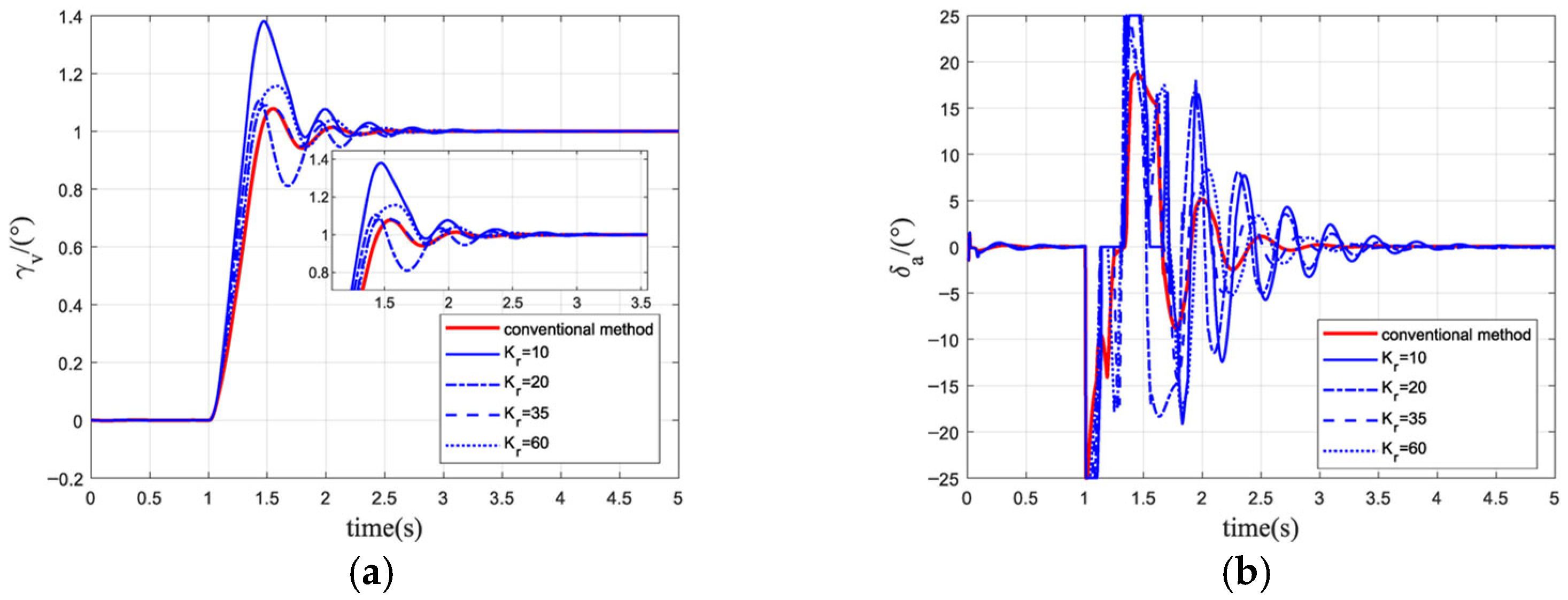
5.1. Simulation Analysis of The Parametric Command Method

In this part, comparisons between the parametric command method and the conventional method are given to illustrate the performance of the proposed method.

The step command is used as the attitude angle command to analyze the effect of command parameters on the performance of the system, without considering the influence of deviations in aerodynamic parameters and disturbances. In addition, the controller parameters are given as $k_1=\mathrm{diag}(15,5)$, $k_2=\mathrm{diag}(20,10)$ and the command parameters are given as $K_p$, $K_r=10$, $20$, $35$, $60$, respectively.

A comparison of the simulation results using the conventional calculation method and the proposed scheme with different parameters is shown in Figure 3 and Figure 4. The simulation results were tallied to obtain the tuning time $t_s$ (the minimum time required for the output response to reach and stay within the 2% error band of its steady-state value), the overshoot $\sigma \%$, and the steady-state accuracy ${\epsilon }_{\sigma }$ of the command response process for different simulation conditions, as listed in

Table 2. Command tracking performance comparison under different simulation conditions.

Simulation Conditions		ts/s		$\mathit{\sigma }\mathit{\%}$		${\mathit{\epsilon }}_{\mathit{\sigma }}{/}^{\mathit{o}}$
		α	${\gamma }_v$	$\alpha$	${\gamma }_v$	$\alpha$	${\gamma }_v$
Conventional Method		$1.67$	$1.95$	$7\%$	$7\%$	$5.6\times {10}^{-8}$	$1.5\times {10}^{-6}$
Parametric Command Method	10	$2.56$	$2.43$	$9\%$	$38\%$	$2.4\times {10}^{-5}$	$2.9\times {10}^{-5}$
	20	$1.67$	$2.25$	$2.6\%$	$10\%$	$5.6\times {10}^{-9}$	$8.2\times {10}^{-7}$
	35	$1.68$	$1.90$	$0$	$9\%$	$2.6\times {10}^{-8}$	$1.1\times {10}^{-6}$
	60	$1.71$	$2.15$	$0$	$16\%$	$2.4\times {10}^{-8}$	$1.2\times {10}^{-6}$

. The smaller the command parameters $K_p$ and $K_r$, the greater the overshoot in the command response process, the greater the rudder deflection angle output by the actuator, and the stronger the dynamic response capability of the control system. With the increase in $K_p$ and $K_r$, the basic change trend of the adjustment time and accuracy of the attitude angle command response is firstly decreased and then increased. When $K_p$ and $K_r$ are 20 and 35, respectively, the response time and control accuracy reach the minimum. Therefore, by optimizing the command parameters $K_p$ and $K_r$, the best performance of the system can be obtained. Comparing the simulation results obtained by command parameters $K_p=20$ and $K_r=35$ with the conventional method, the parametric command method proposed in this paper improves the command response speed, shortens the corresponding process time, and controls the command tracking error to near zero in a shorter time.

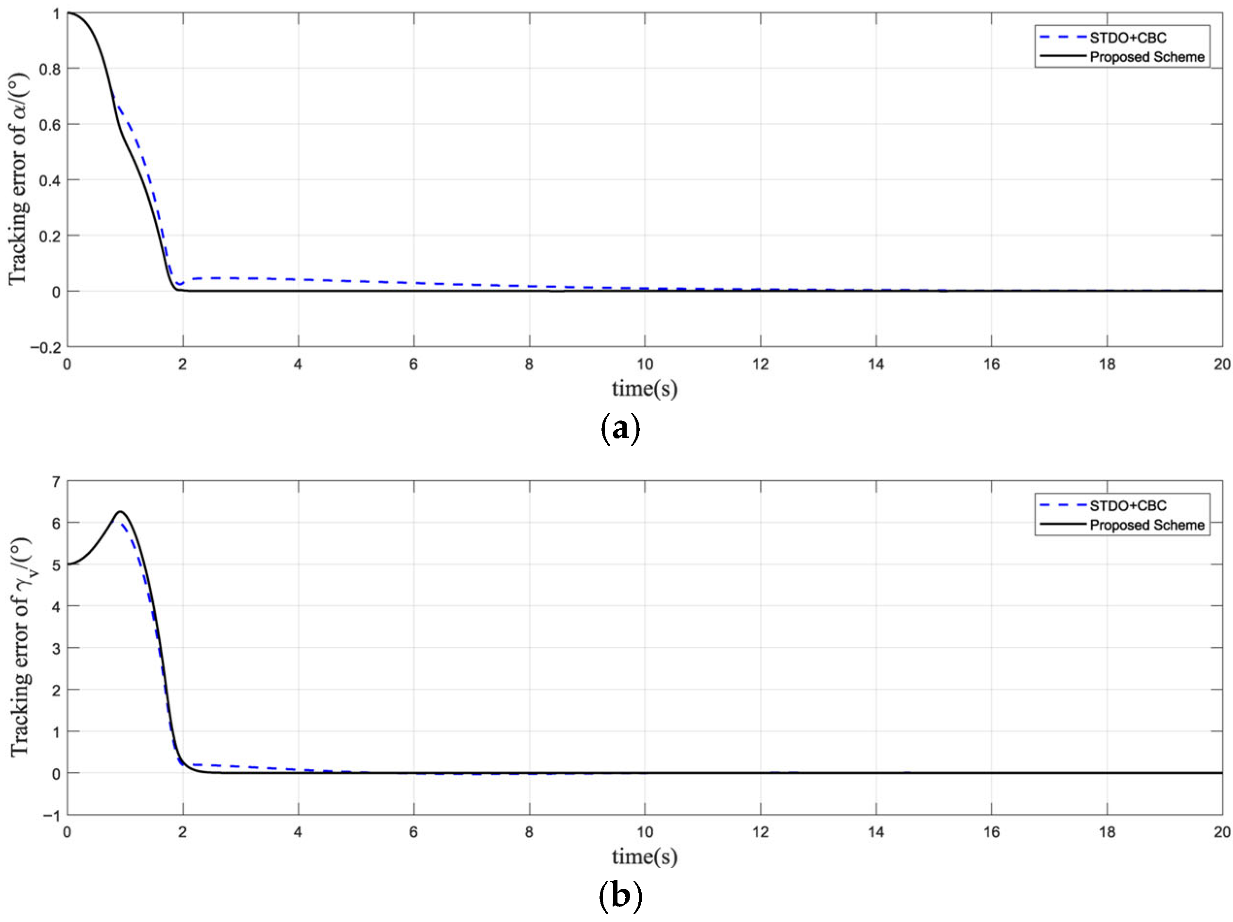
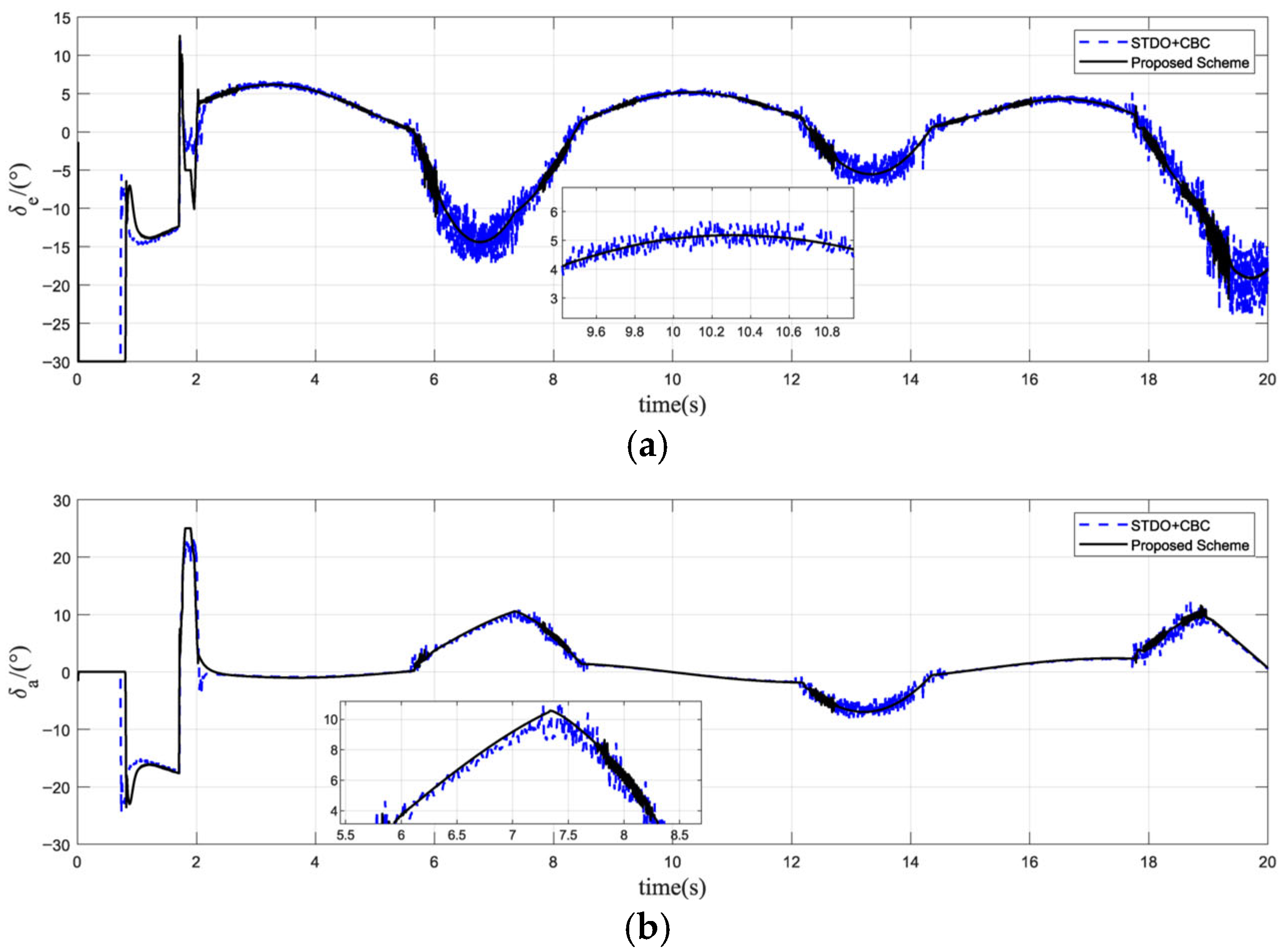
5.2. Simulation Analysis of The Proposed Control Scheme

In this part, simulations of the proposed scheme are shown while taking equivalent disturbances into consideration. Comparisons between the STDO-based backstepping control scheme proposed in this paper and the STDO-based conventional backstepping control scheme mentioned in Zong et al. [33] are given to show the performance of the proposed scheme in this paper. The parameters of the two controllers are listed in

Table 3. Controller parameters.

Controllers	Parameters
STDO-BC	$k_{11}=k_{12}=10$$, k_{21}=k_{22}=5$$, {\mu }_{11}={\mu }_{12}=0.6$$, {\mu }_{21}={\mu }_{22}=0.2$ $k_1=\mathrm{diag}(15,5)$$, k_2=\mathrm{diag}(20,10)$$, K_p=20$$, K_r=35$ ${\tau }_1={\tau }_2=0.01$$, {\zeta }_{f1}={\zeta }_{f2}={\epsilon }_{f1}={\epsilon }_{f2}=0.005$
STDO-CBC	$k_{11}=k_{12}=0.3449$$, k_{21}=k_{22}=0.001,$ $k_{31}=k_{32}=0.1052$$, k_{41}=k_{42}=0.0082$ $k_1=\mathrm{diag}(15,5)$$, k_2=\mathrm{diag}(20,10)$

.

The desired attitude commands are given by:

$$\frac{{\alpha }_c}{{\alpha }_d}=\frac{0.2}{s^2+0.8s+0.16}+6$$

(37)

$$\frac{{\gamma }_{v_c}}{{\gamma }_{v_d}}=\frac{0.3}{s^2+0.8s+0.5}+5$$

(38)

where ${\alpha }_d=6^{\circ }$ and ${\gamma }_{v_d}=5^{\circ }$.

The equivalent disturbance terms are formulated as follows:

$$\begin{array}{l}{d}_{11}=0.03\sin (0.3\pi t) \mathrm{rad}/\mathrm{s}\\ d_{21}=d_{22}=0.02\sin (0.25\pi t) \mathrm{Nm}\end{array}$$

(39)

The tracking curves of the attitude angles and their tracking error curves are shown in Figure 5 and Figure 6, respectively. It can be seen that both control schemes exhibit satisfactory performance in the presence of disturbances, and the control scheme proposed in this paper can guarantee the tracking results with a faster convergence time. The curves of the control variables elevator deflection angle ${\delta }_e$ and roll deflection ${\delta }_a$ are shown in Figure 7. It can be observed that due to the existence of the disturbance observer, both methods have oscillations, but the scheme proposed in this paper has a smaller oscillation amplitude and is smoother.

The different performances of control inputs in Figure 7 and observer errors in Figure 8 between the two control schemes should be discussed. Due to the sign function appearing directly in the conventional STDO, server chattering phenomena may occur when the observation errors converge in the neighborhood of zero, which may cause serious flight accidents in practical applications. For the STDO in this paper, the sign function is hidden in the integral terms, and chattering will be effectively weakened. Thus, the curves of the control input are smoother. It can also be observed that the estimation errors of the STDO proposed in this paper are smaller than that of the STDO in [33]. Therefore, the proposed STDO can effectively improve the robustness of the controller and is more conducive to engineering applications.

6. Conclusions

This paper mainly focuses on the underactuated attitude control problem of a body-flap hypersonic vehicle. A simplified control-oriented model is first introduced. A finite-time super twisting disturbance observer (STDO) is then designed to estimate the equivalent disturbance to the BFHSV, which effectively enhances the anti-disturbance performance of the control scheme. Additionally, a second-order filter is employed to avoid the “explosion of terms” inherent in the conventional backstepping method. In order to enhance the dynamic response of the system, we introduce a parametric command method in the backstepping controller. The stability of the overall system is then demonstrated by utilizing the Lyapunov method. Simulation results illustrate the effectiveness of the control scheme proposed in this paper. In future work, we will extend the derived results for practical applications and control of slide angle.

References

1. Walker, S.; Sherk, J.; Shell, D.; Schena, R.; Bergmann, J.; Gladbach, J. The DARPA/AF Falcon Program: The Hypersonic Technology Vehicle #2 (HTV-2) Flight Demonstration Phase. In Proceedings of the 15th AIAA International Space Planes and Hypersonic Systems and Technologies Conference, Dayton, OH, USA, 28 April 2008; American Institute of Aeronautics and Astronautics: Reston, VA, USA, 2008. [Google Scholar]
2. Wright, D. Research Note to Hypersonic Boost-Glide Weapons by James M. Acton: Analysis of the Boost Phase of the HTV-2 Hypersonic Glider Tests. Sci. Glob. Secur. 2015, 23, 220–229. [Google Scholar] [CrossRef]
3. Wang, F.; Wen, L.; Zhou, C.; Hua, C. Adaptive Preassigned-Time Controller Design for a Hypersonic Vehicle with Improved Performance and Uncertainties. ISA Trans. 2023, 132, 309–328. [Google Scholar] [CrossRef] [PubMed]
4. Zhao, D.; Jiang, B.; Yang, H. Backstepping-Based Decentralized Fault-Tolerant Control of Hypersonic Vehicles in PDE-ODE Form. IEEE Trans. Autom. Control 2022, 67, 1210–1225. [Google Scholar] [CrossRef]
5. Wang, G.; An, H.; Wang, Y.; Xia, H.; Ma, G. Intelligent Control of Air-Breathing Hypersonic Vehicles Subject to Path and Angle-of-Attack Constraints. Acta Astronaut. 2022, 198, 606–616. [Google Scholar] [CrossRef]
6. Xu, B.; Shi, Z. An Overview on Flight Dynamics and Control Approaches for Hypersonic Vehicles. Sci. China Inf. Sci. 2015, 58, 1–19. [Google Scholar] [CrossRef]
7. Ding, Y.; Wang, X.; Bai, Y.; Cui, N. Global Smooth Sliding Mode Controller for Flexible Air-Breathing Hypersonic Vehicle with Actuator Faults. Aerosp. Sci. Technol. 2019, 92, 563–578. [Google Scholar] [CrossRef]
8. Li, X.; Zhang, Z.; An, J.; Zhou, X.; Hu, G.; Zhang, G.; Man, W. Adaptive Sliding Mode Control of Modular Self-Reconfigurable Spacecraft with Time-Delay Estimation. Def. Technol. 2022, 18, 2170–2180. [Google Scholar] [CrossRef]
9. Yang, Z.; Mao, Q.; Dou, L.; Zong, Q.; Yang, J. Composite Design of Disturbance Observer and Reentry Attitude Controller: An Enhanced Finite-Time Technique for Aeroservoelastic Reusable Launch Vehicles. Int. J. Control Autom. Syst. 2022, 20, 2459–2473. [Google Scholar] [CrossRef]
10. Jiang, S.; Tian, F.; Sun, S.; Liang, W. Integrated Guidance and Control of Guided Projectile with Multiple Constraints Based on Fuzzy Adaptive and Dynamic Surface. Def. Technol. 2020, 16, 1130–1141. [Google Scholar] [CrossRef]
11. Zhang, C.; Ahn, C.K.; Wu, J.; He, W. Online-Learning Control with Weakened Saturation Response to Attitude Tracking: A Variable Learning Intensity Approach. Aerosp. Sci. Technol. 2021, 117, 106981. [Google Scholar] [CrossRef]
12. Zhang, C.; Xiao, B.; Wu, J.; Li, B. On Low-Complexity Control Design to Spacecraft Attitude Stabilization: An Online-Learning Approach. Aerosp. Sci. Technol. 2021, 110, 106441. [Google Scholar] [CrossRef]
13. Zhang, C.; Ahn, C.K.; Wu, J.; He, W.; Jiang, Y.; Liu, M. Robustification of Learning Observers to Uncertainty Identification via Time-Varying Learning Intensity. IEEE Trans. Circuits Syst. II Express Briefs 2022, 69, 1292–1296. [Google Scholar] [CrossRef]
14. Isidori, A. Nonlinear Control Systems II. In Communications and Control Engineering; Springer London: London, UK, 1999; ISBN 978-1-4471-1160-3. [Google Scholar]
15. Ye, L.; Tian, B.; Liu, H.; Zong, Q.; Liang, B.; Yuan, B. Anti-Windup Robust Backstepping Control for an Underactuated Reusable Launch Vehicle. IEEE Trans. Syst. Man Cybern. Syst. 2022, 52, 1492–1502. [Google Scholar] [CrossRef]
16. Wang, Z.; Bao, W.; Li, H. Second-Order Dynamic Sliding-Mode Control for Nonminimum Phase Underactuated Hypersonic Vehicles. IEEE Trans. Ind. Electron. 2017, 64, 3105–3112. [Google Scholar] [CrossRef]
17. Moul, M.T.; Paulson, J.W. Dynamic Lateral Behavior of High-Performance Aircraft 1958. Available online: https://ntrs.nasa.gov/citations/19710069982 (accessed on 6 August 2013).
18. Lei, R.-H.; Chen, L. Finite-Time Tracking Control and Vibration Suppression Based on the Concept of Virtual Control Force for Flexible Two-Link Space Robot. Def. Technol. 2021, 17, 874–883. [Google Scholar] [CrossRef]
19. Wei, Y.; Deng, H.; Pan, Z.; Li, K.; Chen, H. Research on a Combinatorial Control Method for Coaxial Rotor Aircraft Based on Sliding Mode. Def. Technol. 2022, 18, 280–292. [Google Scholar] [CrossRef]
20. Ji, P.; Min, F.; Zhang, F.; Ma, F. Tele-Aiming Control Design for Reconnaissance Robot Using a Strong Tracking Multi-Model Extended Super-Twisting Observer. IET Control Theory Appl. 2023, 17, 696–712. [Google Scholar] [CrossRef]
21. Liu, Y.-C.; Laghrouche, S.; Depernet, D.; N’Diaye, A.; Djerdir, A.; Cirrincione, M. Super-Twisting Sliding-Mode Observer-Based Model Reference Adaptive Speed Control for PMSM Drives. J. Frankl. Inst. 2023, 360, 985–1004. [Google Scholar] [CrossRef]
22. Hu, X.; Guo, C.; Hu, C.; He, B. Sliding Mode Learning Control for T-S Fuzzy System and an Application to Hypersonic Flight Vehicle. Asian J. Control 2023, 25, 407–417. [Google Scholar] [CrossRef]
23. Huang, S.; Jiang, J.; Li, O. Sliding Mode Backstepping Control for the Ascent Phase of Near-Space Hypersonic Vehicle Based on a Novel Triple Power Reaching Law. Aerospace 2022, 9, 755. [Google Scholar] [CrossRef]
24. Ju, X.; Wei, C.; Xu, H.; Wang, F. Fractional-Order Sliding Mode Control with a Predefined-Time Observer for VTVL Reusable Launch Vehicles under Actuator Faults and Saturation Constraints. Isa Trans. 2022, 129, 55–72. [Google Scholar] [CrossRef] [PubMed]
25. Zhang, X.; Hu, W.; Wei, C.; Xu, T. Nonlinear Disturbance Observer Based Adaptive Super-Twisting Sliding Mode Control for Generic Hypersonic Vehicles with Coupled Multisource Disturbances. Eur. J. Control 2021, 57, 253–262. [Google Scholar] [CrossRef]
26. Gurumurthy, G.; Das, D.K. Terminal Sliding Mode Disturbance Observer Based Adaptive Super Twisting Sliding Mode Controller Design for a Class of Nonlinear Systems. Eur. J. Control 2021, 57, 232–241. [Google Scholar] [CrossRef]
27. Snell, S.A.; Enns, D.F.; Garrard, W.L. Nonlinear Inversion Flight Control for a Supermaneuverable Aircraft. J. Guid. Control Dyn. 1992, 15, 976–984. [Google Scholar] [CrossRef]
28. Wang, Z.; Li, H.; Bao, W. Body-flap attitude control method for lifting re-entry vehicle. J. Beijing Univ. Aeronaut. Astronaut. 2016, 42, 532–541. [Google Scholar] [CrossRef]
29. Li, Z.; Zhai, J. Super-twisting Sliding Mode Trajectory Tracking Adaptive Control of Wheeled Mobile Robots with Disturbance Observer. Int. J. Robust Nonlinear Control 2022, 32, 9869–9881. [Google Scholar] [CrossRef]
30. Mei, K.; Ding, S.; Yu, X. A Generalized Supertwisting Algorithm. IEEE Trans. Cybern. 2023, 53, 3951–3960. [Google Scholar] [CrossRef]
31. Zhao, J.; Feng, D.; Cui, J.; Wang, X. Finite-Time Extended State Observer-Based Fixed-Time Attitude Control for Hypersonic Vehicles. Mathematics 2022, 10, 3162. [Google Scholar] [CrossRef]
32. Li, C.-Y.; Jing, W.-X.; Gao, C.-S. Adaptive Backstepping-Based Flight Control System Using Integral Filters. Aerosp. Sci. Technol. 2009, 13, 105–113. [Google Scholar] [CrossRef]
33. Zong, Q.; Dong, Q.; Wang, F.; Tian, B. Super Twisting Sliding Mode Control for a Flexible Air-Breathing Hypersonic Vehicle Based on Disturbance Observer. Sci. China Inf. Sci. 2015, 58, 1–15. [Google Scholar] [CrossRef]
Figure 1. (a) Three-dimensional view of the BFHSV; (b) bottom view of the BFHSV.
Mathematics 11 02460 g001
Figure 2. Overall structure diagram of control scheme.
Mathematics 11 02460 g002
Figure 3. (a) Response process of the angle of attack with different command parameters; (b) response process of the elevator with different command parameters.
Mathematics 11 02460 g003
Figure 4. (a) Response process of the bank angle with different command parameters; (b) response process of the roll rudder with different command parameters.
Mathematics 11 02460 g004
Figure 5. (a) Tracking curve of α ; (b) tracking curve of γ v .
Mathematics 11 02460 g005
Figure 6. (a) Tracking error curve of α ; (b) tracking error curve of γ v .
Mathematics 11 02460 g006
Figure 7. (a) Control input curve of δ e ; (b) control input curve of δ a .
Mathematics 11 02460 g007
Figure 8. (a) Observer error curve of d 11 ; (b) observer error curve of d 21 ; (c) observer error curve of d 22 .
Mathematics 11 02460 g008aMathematics 11 02460 g008b