DNN-MLVEM: A Data-Driven Macromodel for RC Shear Walls Based on Deep Neural Networks

Abstract

This study proposes the DNN-MVLEM, a novel macromodel for the non-linear analysis of RC shear walls based on deep neural networks (DNN); while most RC shear wall macromodeling techniques follow a deterministic approach to find the right configuration and properties of the system, in this study, an alternative data-driven strategy is proposed instead. The proposed DNN-MVLEM is composed of four vertical beam-column elements and one horizontal shear spring. The beam-column elements implement the fiber section formulation with standard non-linear uniaxial material models for concrete and steel, while the horizontal shear spring uses a multi-linear force–displacement relationship. Additionally, three calibration factors are introduced to improve the performance of the macromodel. The data-driven component of the proposed strategy consists of a large DNN that is trained to predict the force–displacement curve of the shear spring and the three calibration factors. The training data is created using a parametric microscopic FEM model based on the multi-layer shell element formulation and a genetic algorithm (GA) that optimizes the response of the macromodel to match the behavior of the microscopic FEM model. The DNN-MVLEM is tested in two types of examples, first as a stand-alone model and then as part of a two-bay multi-story frame structure. The results show that the DNN-MVLEM is capable of reproducing the results obtained with the microscopic FEM model up to 100 times faster and with an estimated error lower than 5%.

1. Introduction

The modeling of reinforced concrete (RC) shear walls is an essential area of research in earthquake engineering [1]. Engineers have sought to create numerical models of RC shear walls that can be reliably used for the analysis and design of structures under earthquake hazards [2,3]. Over the years, the research and development of modeling strategies have resulted in two main distinguished categories: macroscopic and microscopic models [4].

Microscopic modeling (micromodels) strategies attempt to create a model with an elevated level of detail and refinement to reproduce the complex interaction between the concrete and the reinforcement steel at a microscopic level [5,6]. The most popular micromodeling technique is the implementation of finite element method (FEM) models utilizing solid, shell, and beam/truss elements combined with state-of-the-art material models for concrete and reinforcement steel [7,8,9]. One such example is the 3D FEM model developed by Fei-Yu et al. [10], where each reinforcement bar is modeled independently, including the corresponding contact interaction between steel and concrete. Micromodels stand out for their good performance in reproducing the realistic behavior of RC shear walls [11]. Their effectiveness has been extensively demonstrated in various studies [12,13,14,15]. However, their main disadvantage is their high computational cost, significantly reducing their practical applicability for the analysis of large-scale real-world structures. For example, the model in Figure 1 contains more than 100,000 degrees of freedom and takes 22 h to run 100 steps of a static non-linear pushover analysis on four cores with a computer equipped with an Intel Core i7-6700HQ CPU @2.60 GHz.

Macroscopic modeling (macromodels) techniques, on the other hand, attempt to reproduce the overall behavior of RC shear walls at the macro scale with a much simpler model [16]; thus, their computational cost is significantly lower. These models typically combine springs and axial bars connected through rigid elements to mimic the wall geometry. They implement non-linear material laws for both the concrete and the reinforcement steel. However, the shear and flexural response in these systems is usually uncoupled, meaning that the element can experience shear and flexure deformations independently, which is normally not physically possible. Hence, their efficacy to model certain effects is limited [17]. Nonetheless, the research and development of macromodeling techniques is a popular and active area of research as the analysis and design paradigm is shifting towards performance-based techniques [18], where the assessment of the non-linear behavior of the structure plays a central role. Therefore, creating reliable macromodels that contribute to reducing the computational cost of the non-linear analysis of structures is of particularly high interest.

Macroscopic modeling techniques have been around for a few decades; among the first proposed macromodels is the three-vertical-line-element model by Kabeyasawa et al. [19]. It consists of two axial springs, one rotational spring for flexure, and one horizontal spring for shear deformation; see Figure 2a. Vulcano et al. [20,21] improved the model by removing the rotational spring and using several vertical axial fibers in parallel instead, creating the multiple-vertical-lines-element-model (MVLEM); see Figure 2b. Since then, the MVLEM has become widely popular and has been thoroughly tested and verified in numerous studies [22,23,24,25,26]. The MVLEM has also been included in various popular FEM packages, such as in the OpenSees framework [27]. Additionally, it has served as the base and motivation for developing similar models with enhanced properties, such as the SFI-MVLEM [28,29] depicted in Figure 2c, the V-MVLEM [30], and others [31,32].

Despite the efforts to find the perfect macromodel, some of their disadvantages are too difficult to overcome due to the underlying assumptions and simplifications implicit in their formulations. For instance, they may be unable to fully capture the RC shear wall’s complex behavior to its full extent. A comparative study by Kolozvari et al. [17] found that some macromodels were not reliable in predicting the local strains at the base (where the higher strains are localized). In such cases, the tensile strains were overestimated as much as a factor of 2.0, while the compressive strains were underestimated up to 2.0–3.0 times. Overall, RC shear walls’ behavior is a complex phenomenon challenging to model using simplified methods based on deterministic strategies. Deterministic methods usually cannot capture complex phenomena to their full extent, becoming subject to many limitations that restrict their applicability. In contrast, data-driven strategies that do not follow the deterministic road have proven to be a better alternative for complex problems [33], provided that sufficient and high-quality data are used in their formulation.

In this study, a novel data-driven macromodel for modeling RC shear walls is developed based on deep learning techniques. The macromodel, referred to as DNN-MVLEM, is composed of four vertical beam-column elements that implement the fiber section formulation and a non-linear horizontal shear spring. All the elements are connected together with rigid elements to mimic the RC shear wall geometry. The material models for the vertical elements are based on well-established non-linear models commonly used for concrete and reinforcement steel. For the shear spring, a multi-linear material model is implemented. The final piece of the macromodel is three factors that are introduced to calibrate it and improve its accuracy. The data-driven component of the macromodel consists of a deep neural network (DNN) trained in a two-phase procedure. In the first phase, the DNN is trained to predict the force–displacement curve to define the multi-linear curve for the shear spring material model. To that end, a parametric microscopic FEM model generates the corresponding data. In the second phase, several macromodels are built and calibrated to match the results of the microscopic FEM model using a genetic algorithm (GA). The results are used to re-train the DNN to add the calibration factors to its predictions. Hence, the final DNN is able to predict all the required information to construct the macromodel.

The DNN-MVLEM is a novel approach inspired by the effectiveness of data-driven strategies to substitute intricate hard-computing models for solving complex problems with reliable approximations that require significantly less computational effort. Notably, in structural engineering [34], these strategies are quickly gaining momentum and acceptance for both research and industrial applications [35]. Several recent examples can be found, such as the following: using artificial neural networks (ANN) to predict the lateral capacity of RC shear walls [36]; predicting the non-linear response of 3D buildings under seismic actions with ANNs [37]; using ANNs as non-linear constitutive materials [38]; autonomous design of structures using optimization algorithms [39,40,41,42]; speeding up the solution procedure of FEM equations [43,44]; surrogate modeling of large FEM structures [45,46,47]; using the ensemble wavelet-neural networks [48] and physical informed neural networks (PINN) [49] to estimate the properties of complex materials such as concrete composites; and many other exciting applications [50,51].

The remainder of the paper is organized as follows. Section 2 presents the basic structure and components of the DNN-MVLEM. Section 4 explains the data-driven component of the model, which includes a description of the microscopic FEM model used for the data generation. Section 5 presents various numerical examples of the DNN-MVLEM compared to the microscopic FEM model. Finally, the results are discussed in Section 6, and the conclusions are presented in Section 7.

2. The DNN-MVLEM

2.1. Base Elements

The DNN-MLVEM has been implemented using the FEM framework provided by the OpenSeesPy library [52,53]. It is composed of four vertical columns—two columns $K_{eb1}$ and $K_{eb2}$ for the boundary elements, and another two $K_{web1}$ and $K_{web2}$ for the web part of the wall. Each of the columns is positioned at the center of the tributary area of the portion of the wall that is intended to represent. Additionally, to simulate the shear resistance, there is a horizontal axial spring $S_h$ in the middle of the model positioned at a distance of 0.4 h from the bottom. The whole system is held together by rigid beam elements. The resulting configuration of the macromodel is depicted in Figure 3.

The columns are modeled using beam-column elements with the fiber section formulation [54]. Their corresponding commands in OpenSees are the “forceBeamColumn” element and the “fiber” section. For the four vertical elements, the cross-section is discretized into 20 rectangular fibers in the direction of the wall length for the concrete area. The total quantity for the reinforcement steel is distributed into six fibers, with four positioned in the corners and two in the middle of the larger edges. Figure 3b depicts the resulting fiber section. The shear spring $S_h$ consists of a uni-axial element that provides only stiffness in the horizontal direction, modeled using the “zeroLenght” element in OpenSees. The rigid beams at the top and bottom of the macromodel and the additional elements holding the shear spring are modeled using the “elasticBeamColumn” element command with a large cross-section assigned to simulate the rigid behavior.

2.2. Material Models for Vertical Elements

The material model for the concrete fibers in the columns is the Kent–Scott–Park model, which does not include tensile strength in its formulation. It is denoted as “Concrete01” in OpenSees, and its definition requires four parameters: the concrete compressive strength $f_c^{\prime }$; the strain at the maximum compressive strength ${ϵ}_{co}$, taken as −0.002; the crushing strength $f_{cu}$, taken as $0.2f_c^{\prime }$; and the strain at the crushing strength ${ϵ}_{cu}$, taken as −0.01. A second concrete material model is defined for the confined regions. The material parameters for the unconfined concrete model are the same as those previously mentioned but with the values of $f_{cu}=0$ and ${ϵ}_{cu}=-0.005$.

For the reinforcement steel fibers in the columns, the Giuffre–Menegotto–Pinto model that includes the characteristic post-yielding and the Bauschinger effects have been used. It is identified as “Steel02” in OpeenSees, and its definition requires three parameters: the yield stress $f_y$; the initial elastic tangent, taken as $E_0=210$ GPa; and the strain-hardening ratio, taken as $b=0.01$ (b is the ratio between the elastic tangent $E_0$ and the post-yield tangent $E_p$).

The values for the material parameters for the concrete and the reinforcement steel sections are taken from well-established studies found in the literature, such as [55,56,57,58,59,60]. A representative stress–strain curve for both material models is presented in Figure 4. Note that the curves are not scaled; their only intention is to provide a visual definition of the required parameters.

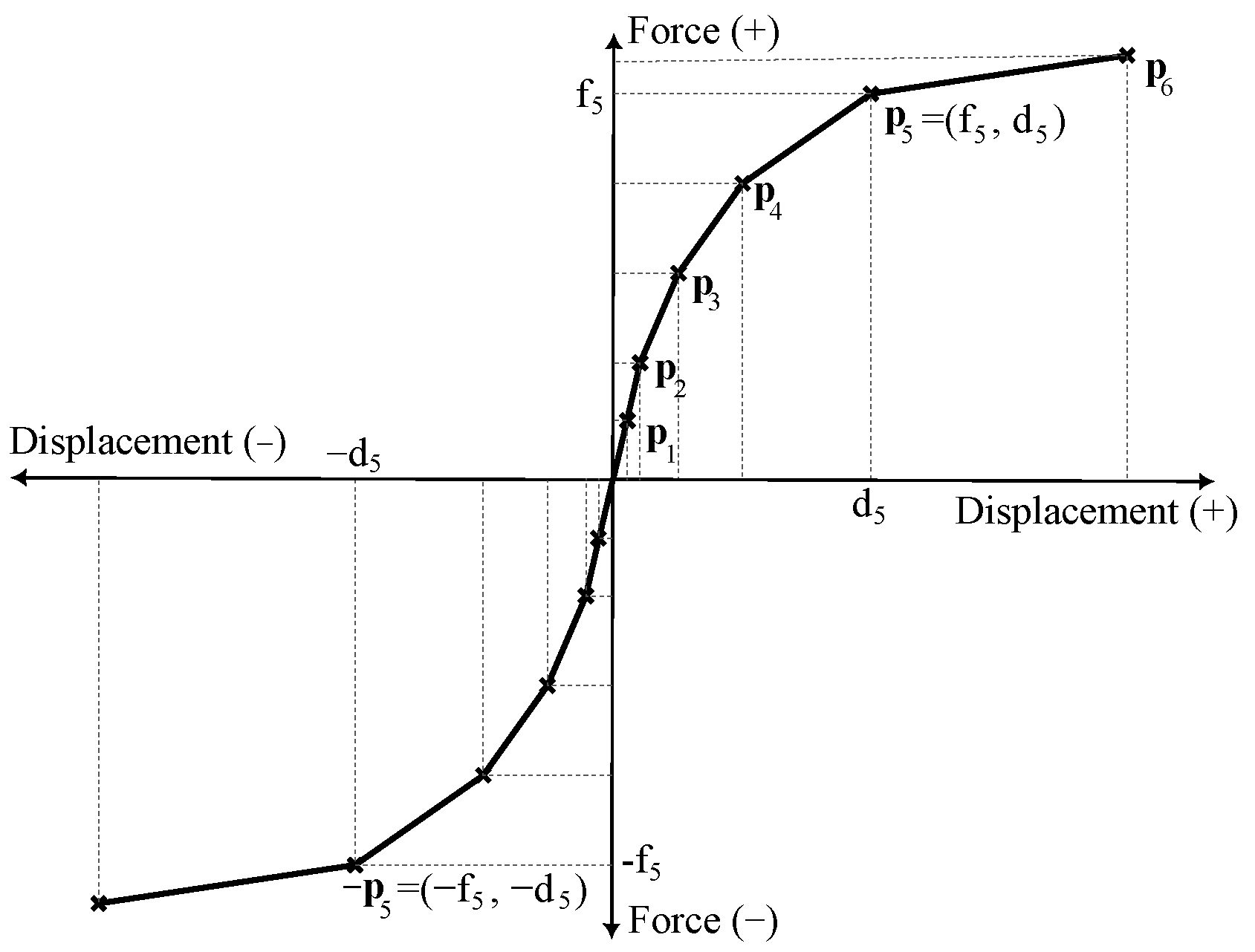
2.3. Material Model for Shear Spring

For the shear spring $S_h$, a multi-linear material is used with the “MultiLinear” uniaxial material command in OpenSees. The force–displacement coordinates of the multi-linear curve are obtained in the following way. Suppose that a more sophisticated FEM model is used to model the RC shear wall and perform a static non-linear lateral pushover analysis. Then, the computed pushover curve (horizontal force–displacement relation measured at the top of the model through the analysis) is discretized into six segments so that six force–displacement coordinates are obtained. These six force–displacement coordinates define the multi-linear material model for the shear spring. A representative force–displacement curve of the multi-linear model is given in Figure 5. Such a curve serves as the basic shape of the multi-linear model that is later calibrated with a process described in Section 4.

Using the pushover curve obtained with FEM analysis as the curve for the multi-linear material may seem counter-intuitive as it implies the solution of a computationally expensive analysis first. However, this is not the case. The six points defining the multi-linear model are obtained by calling a DNN previously trained with thousands of static non-linear pushover FEM analyses of RC shear walls. The complete description of the methodology to develop the DNN is given in Section 4.

2.4. Calibration Factors

The DNN-MVLEM is constructed on top of various assumptions and simplifications, which, depending on multiple parameters such as the geometry and reinforcement quantity, may deviate its performance from the actual behavior of the RC shear wall. Thus, a simple data-driven calibration method has been developed. The strategy consists of using three factors to adjust its behavior, namely $k_c$, $k_s$, and $k_m$. The factor $k_c$ multiplies the thickness t of the cross-sections, while $k_s$ multiplies the strength of reinforcement steel $f_y$. The third factor $k_m$ multiplies the six force coordinates used to define the multi-linear model, shifting the curve up or down.

The calibration is performed by solving an optimization problem using a genetic algorithm. The decision to include these three factors to calibrate the macromodel’s behavior comes after several attempts to improve its accuracy without sacrificing its simplicity or computational efficiency. For instance, instead of adding more elements or implementing more complex material models, the optimization algorithm calibrates its performance by simply adjusting the response with three factors.

In principle, the macromodel is calibrated to match the results of a more sophisticated microscopic FEM model. The strategy may seem paradoxical because it implies computing the solution with an expensive microscopic FEM model to calibrate a simpler macromodel. However, this is where the benefits of the data-driven paradigm are genuinely harnessed. Instead of conducting the calibration process each time the macromodel is used, an extensive database of macromodels is calibrated beforehand. Then, that database is used to train a DNN to predict the calibration factors. Thus, the computationally expensive operation is transferred to an external process where the database is generated, and the DNN model is trained. After those processes are finalized, the DNN becomes ready to be used at any given time, predicting the calibration factors in a few milliseconds. The process is described in more detail in Section 4.

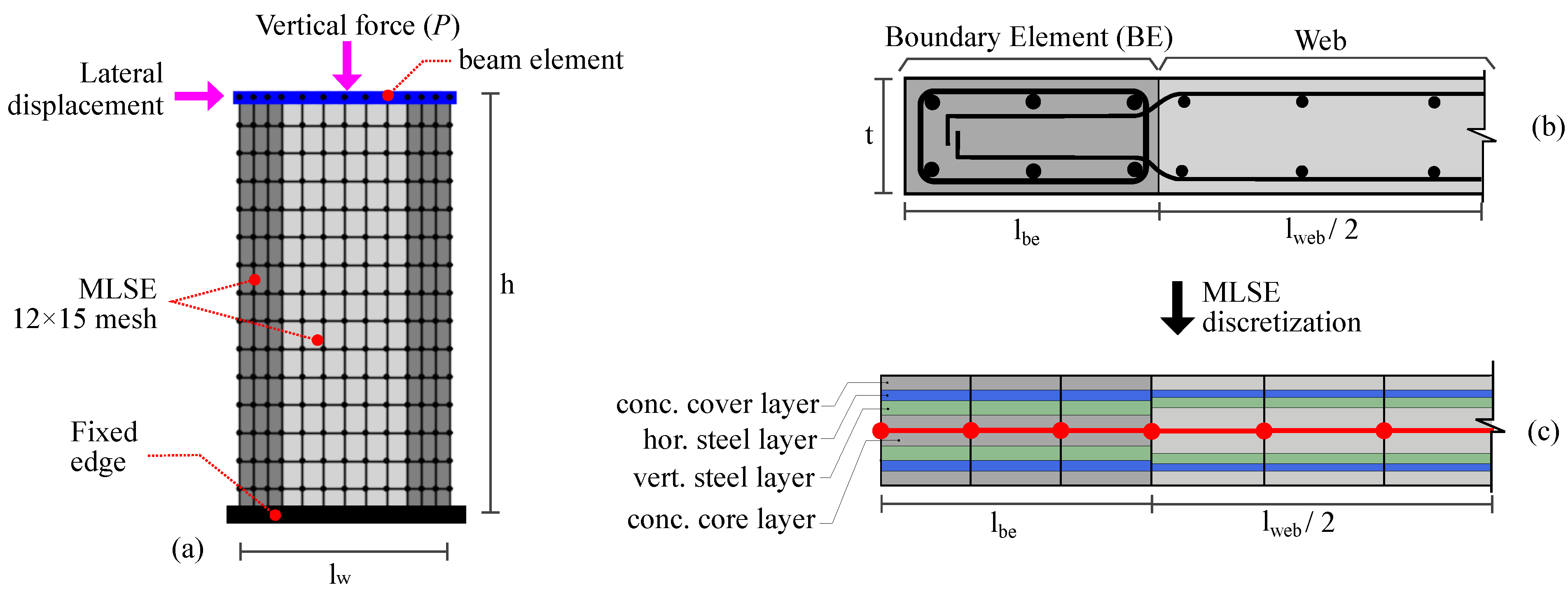
3. Parametric FEM Model for Data Generation

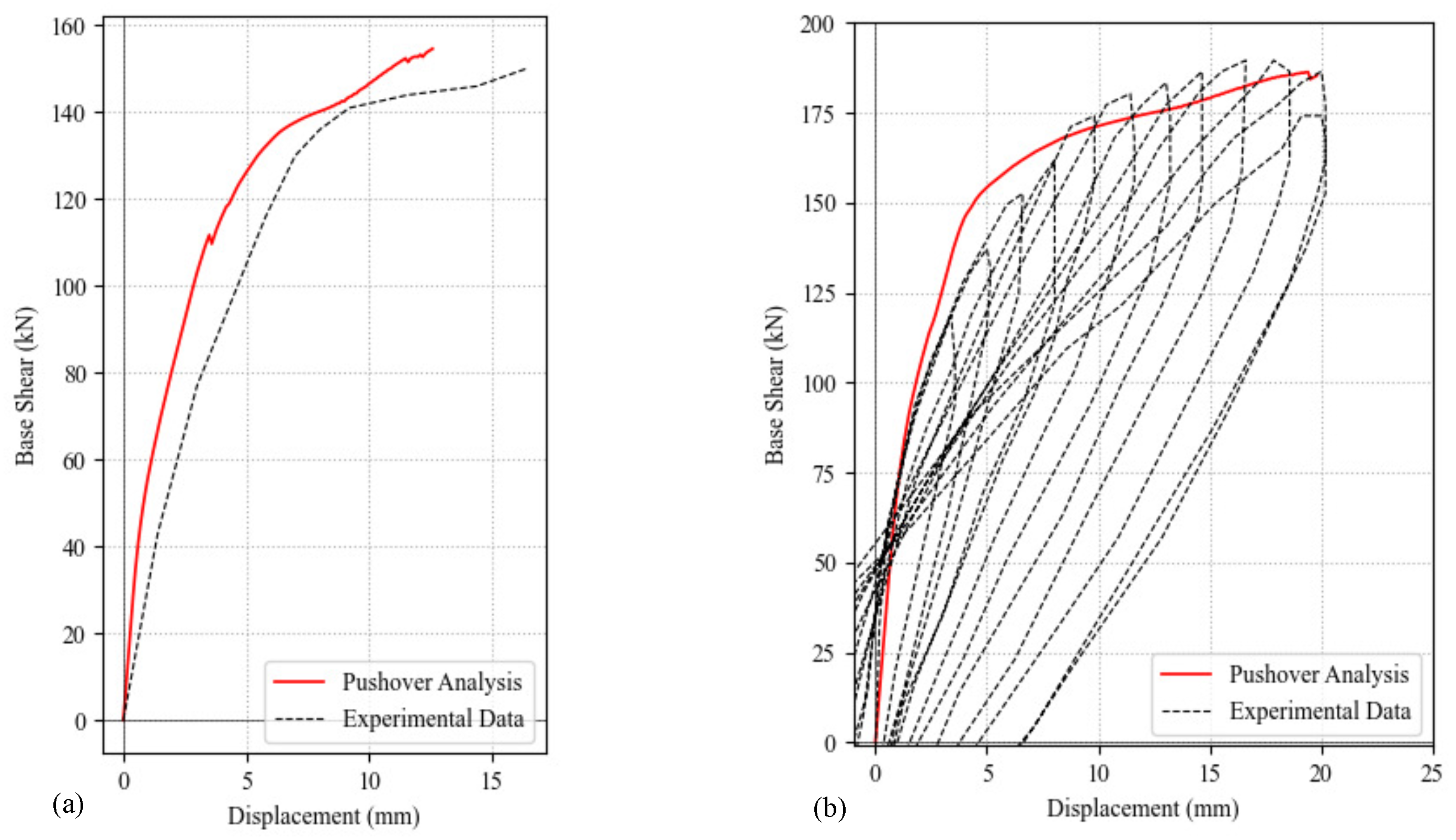
The required data for the DNN-MVLEM methodology are generated using a microscopic FEM model based on the multi-layer shell element (MLSE) formulation, particularly the implementation developed by Lu et al. [61,62]. The MLSE has proven to be an effective and practical modeling approach capable of reproducing the in-plane and out-of-plane bending and the characteristic in-plane shear and coupled bending–shear behavior of RC shear walls [63,64]. In the MLSE approach, the shell thickness is discretized into several fully-bonded layers, including the vertical and transverse reinforcement steel as smeared orthotropic layers.

The model consists of a rectangular RC shear wall with special boundary elements (BE) on both sides with a beam element added at the top to distribute the loads to all the nodes on the top edge. The model is parameterized into 11 different variables that describe the geometry and properties of the wall. These parameters are described in

Table 1. Parameters that define the properties and dimensions of an RC shear wall.

n	Symbol	Lower Bound	Upper Bound	Description
1	$f_c^{\prime }$	25	60	Concrete compressive strength [MPa]
2	$f_y$	380	600	Reinforcing steel yield stress [MPa]
3	h	300	350	Wall height [cm]
4	t	12.5	40	Wall thickness [cm]
5	$l_w$	$t·6$	300	Wall total length [cm]
6	$l_{be}$	0.15$·l_w$	0.30$·l_w$	BE length [cm]
7	${\rho }_{l_{be}}$	0.01	0.05	BE longitudinal reinforcement ratio
8	${\rho }_{t_{be}}$	0.0075	0.02	BE transversal reinforcement ratio
9	${\rho }_{l_{web}}$	0.0025	0.75$·{\rho }_{l_{be}}$	Web longitudinal reinforcement ratio
10	${\rho }_{t_{web}}$	0.0025	0.75$·{\rho }_{t_{be}}$	Web transversal reinforcement ratio
11	$q_a$	0.005	0.1	Axial load ratio, $P=q_a·0.85·f_c^{\prime }·t·l_w$

.

The model is subjected to a two-stage analysis procedure. In the first stage, a vertical load is applied to simulate the gravity actions. In the second stage, a static non-linear lateral pushover analysis with a target displacement of 20 mm applied at the top-left node at a rate of 0.05 per step is conducted. The final form of the model and an illustration of the multi-layer shell element discretization is shown in Figure 6.

The chosen bounding values in Table 1 are derived from design guidelines provided by the American Concrete Institute (ACI318-19) [65] and from engineering criteria. The bounding values are selected to produce realistic wall geometries and configurations. For instance, the ACI318-19 specifies that the minimum thickness allowed for a structural wall is $t=12.5$ cm, and the smallest length-to-thickness ratio is $l_w/t=6$. As a result, the lower bound for the wall length is set to $t·6$. Additionally, Section 18.10.6.4 of the ACI318-19 recommends a transverse reinforcement quantity of ${\rho }_{t_{be}}$ for the boundary element range of 0.0075 to 0.020, depending on the material properties. The longitudinal reinforcement ${\rho }_{l_{be}}$ is similar to concrete columns, so a value between 0.01 and 0.05 is reasonably selected. Note that reinforcement is expressed as a ratio of the corresponding concrete cross-sectional area. The compressive strength $f_c^{\prime }$ and yield strength $f_y$ range from traditional values commonly used in the construction of modern buildings. The wall length $l_w$ and height h are based on typical wall dimensions found in medium-rise buildings. The axial load value $q_a$ is expressed as a ratio of the maximum axial strength for concrete sections according to Equation 22.4.2.2 of ACI318-19. The range of 0.010 to 0.1 is chosen based on the assumption that a value of 0.1 represents the loading of a wall in the bottom story of a medium-height building [66].

3.1. Validation

The selected MLSE approach is validated with two numerical examples by comparing the results to some of the popular experimental tests available in the literature. For the first case, the specimen labeled as SW22 taken from the study conducted by Lefas et al. [66] is selected. The input values are: $f_c^{\prime }=50.6$ MPa, $f_y=470$ MPa, $h=130$ cm, $t=7$ cm, $l_w=65$ cm, $l_{be}=0.215$ (14 cm), ${\rho }_{l_{be}}=0.033$, ${\rho }_{t_{be}}=0.008$, ${\rho }_{l_{web}}=0.025$, ${\rho }_{t_{web}}=0.008$, $q_a=0.1$. The second case corresponds to the specimen SW1-1 taken from the database [67]. The input values are: $f_c^{\prime }=20.7$ MPa, $f_y=392$ MPa, $h=200$ cm, $t=12.5$ cm, $l_w=100$ cm, $l_{be}=0.20$ (20 cm), ${\rho }_{l_{be}}=0.0188$, ${\rho }_{t_{be}}=0.0028$, ${\rho }_{l_{web}}=0.0037$, ${\rho }_{t_{web}}=0.0018$, and $q_a=0.11$. The results for both examples are shown in Figure 7a,b.

The presented numerical examples demonstrate that the implemented RC shear wall FEM model based on the MLSE formulation reproduces the experimental results reasonably, even when two different databases are used. Although only two specimens were analyzed in this study, the same MLSE implementation has been tested extensively in other studies [61,62,68].

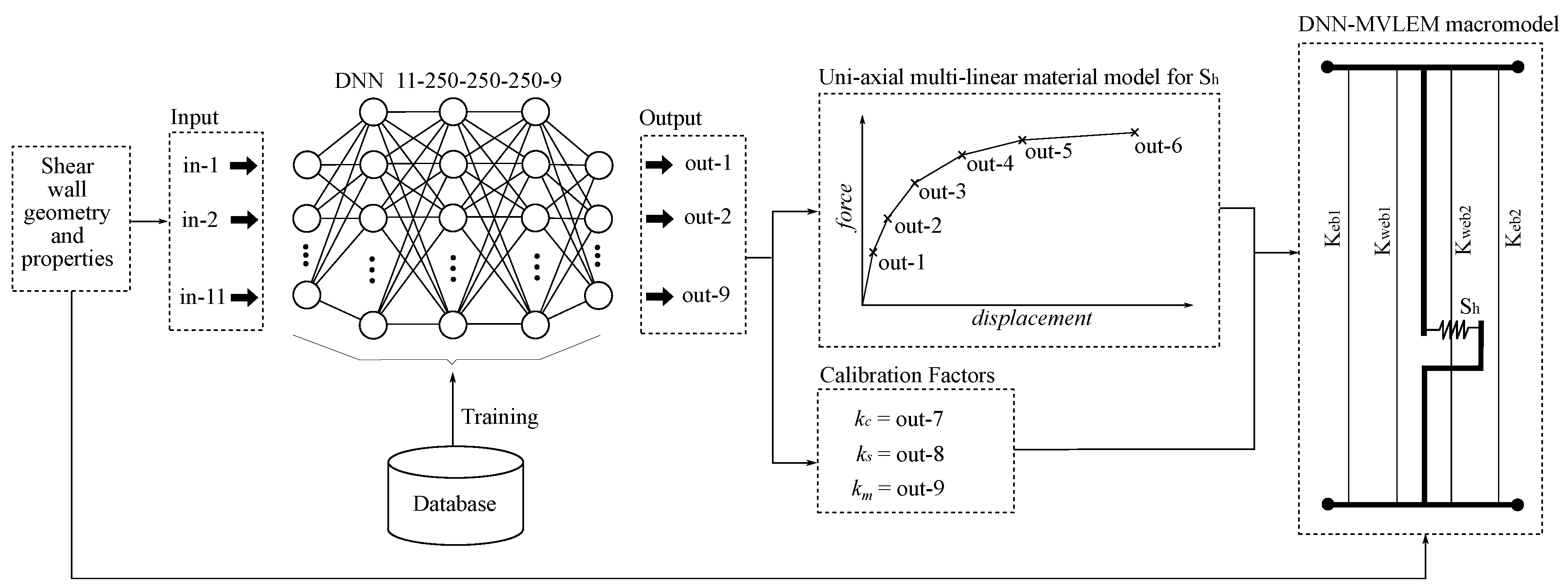
4. Data-Driven Component

The key ingredient of the DNN-MVLEM is adding the data-driven component, which consists of a large deep neural network trained with thousands of non-linear analyses of RC shear walls. The DNN is trained to predict the force–displacement curve for the multi-linear model used in the shear spring and the three factors required to calibrate its performance, as illustrated in Figure 8.

The data-driven component is summarized in eight steps. In the first phase (Steps 1 to 4), a database is generated that contains thousands of RC shear walls and their corresponding analysis results obtained with the FEM model described in Section 3. The database is used to train a temporary DNN to predict the multi-linear model for the shear spring. In the second phase (Steps 5 to 8), for every RC shear wall in the database, the corresponding macromodel is generated and calibrated to match the FEM results using a genetic algorithm. The calibration factors for each data point are added to the initial database so that a second larger DNN is trained to predict the two parts: the multi-linear curve for the shear spring and the calibration factors, thus obtaining a single DNN that predicts the complete information required to define the DNN-MVLEM. The eight steps are described in more detail in the following paragraphs.

Step 1. A vector $\mathbf{w}$ that contains the 11 input values is generated using a uniform random distribution based on the bounding values specified in Table 1. The vector has the following form.

$$\begin{array}{c}\hfill \mathbf{w}=\{f_c^{\prime },f_y,h,t,l_w,l_{be},{\rho }_{l_{be}},{\rho }_{t_{be}},{\rho }_{l_{web}},{\rho }_{t_{web}},q_a\}\end{array}$$

Step 2. The vector $\mathbf{w}$ is used to generate the microscopic FEM model described in Section 3. The model is subjected to a static non-linear lateral pushover analysis. The obtained pushover curve is discretized into six segments by reading the force at the displacement values of 0.5, 1.0, 2.5, 5.0, 10.0, and 20.0 mm. Step 2 can be conveniently summarized into a single function as:

$$\begin{array}{c}\hfill p\left(\mathbf{w}\right)=\{p_1,\dots ,p_6\}\end{array}$$

(1)

where $p_i$ are the force coordinates of the discretized pushover curve obtained with the microscopic FEM model.

Step 3. Steps 1 and 2 are repeated several times until a large database of analysis results is generated. The database is denoted as 11 × 6 because it contains 11 input and 6 output values per data point.

Step 4. A temporary DNN, referred to as DNNb, is created and trained with the 11 × 6 database; thus, obtaining a DNN that predicts the 6 values corresponding to the 6 force coordinates of the discretized pushover curve.

Step 5. From the 11 × 6 database, a data point is selected, and the 11 input values are used to build the corresponding macromodel according to the process described in Section 2. The DNNb is used to obtain the force–displacement curve of the shear spring $S_h$, and the calibration coefficients are set to an initial value of $k_c=k_s=k_m=1$. Similarly to Step 2, the following function is defined:

$$\begin{array}{c}\hfill q(\mathbf{w},k_c,k_s,k_m)=\{q_1,\dots ,q_6\}\end{array}$$

(2)

where $q_i$ are the force coordinates of the discretized pushover curve obtained with the macromodel after performing the same static pushover analysis, and applying the same six-value discretization as in Step 2.

Step 6. The calibration procedure is formulated as an optimization problem:

$$\begin{array}{cc}\hfill \min e=|& p\left(\mathbf{w}\right)-q(\mathbf{w},k_c,k_s,k_m)|\hfill \\ \hfill \\ \hfill 0.1\le & k_c\le 2k_c\in \mathbb{R}\hfill \\ \hfill 0.1\le & k_s\le 2k_s\in \mathbb{R}\hfill \\ \hfill 0.1\le & k_m\le 5k_m\in \mathbb{R}\hfill \end{array}$$

(3)

The calibration coefficients are computed by solving the optimization problem with a genetic algorithm. To that end, the genetic algorithm in the multi-objective optimization Python library known as “pymoo” [69] is used. The GA is run for a total of 50 generations using the default parameters provided by the library, which include a population size of 100 and the genetic operators of SBX crossover, polynomial mutation, and tournament selection. The optimization problem is unconstrained, but the solution vector is limited to the space dictated by the bounding values of the variables $k_c,k_s,k_m$.

Step 7. Steps 5 and 6 are repeated until the calibration coefficients of all the RC shear walls in the database are computed, obtaining a larger 11 × 9 database with nine output values (the six values obtained in Step 2 and the three values obtained in Step 6).

Step 8. With the 11 × 9 database, a second larger DNN model is created and trained to predict the complete information (the six output values used for the multi-linear model and the three calibration factors). The DNN details, such as the architecture and its performance, are given in Section 4.1.

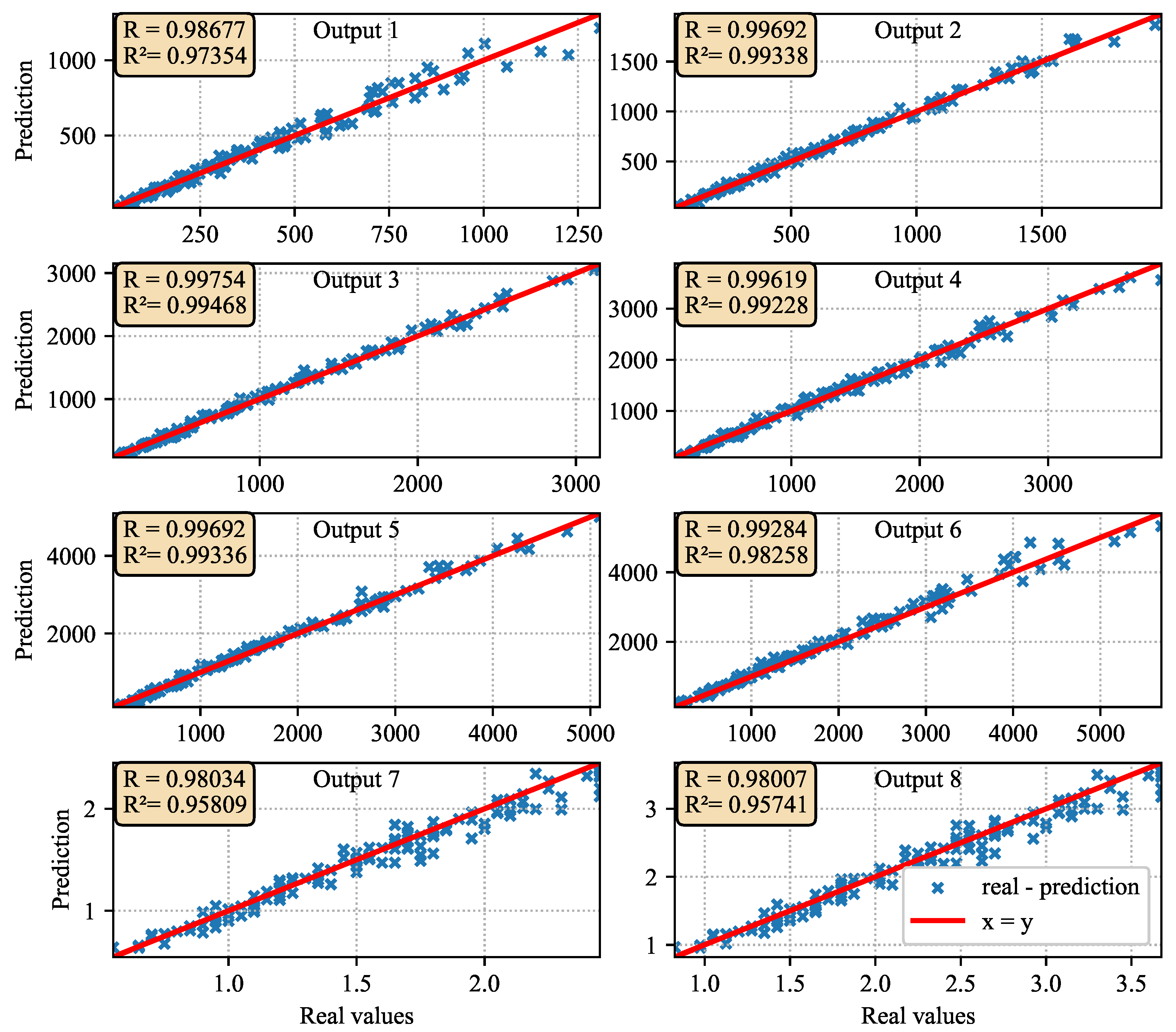
4.1. DNN Architecture and Performance

The DNN has been created using the TensorFlow library [70]. The chosen architecture is a back-propagation neural network with 11 input neurons at the input layer, 3 hidden layers with 250 neurons each, and an output layer with 9 neurons. Its size can be expressed in the following way: $11-250-250-250-9$. The total number of trainable parameters is equal to $(11+1)\times 250+(250+1)\times 200+(250+1)\times 250+(250+1)\times 9=130,759$.

The database is composed of 3000 data points that are generated using the procedure described in Section 4. The inputs and the outputs are normalized to add flexibility and stability to the DNN. A validation subset of 10% of the training data is used to monitor the training process and avoid over-fitting. Other relevant characteristics are the usage of the Adams optimizer, ReLu activation functions, a batch size of 5, and a random uniform initialization of the weights.

After the training, the DNN is tested using a freshly generated data set containing 200 new data points. The testing set is processed by the DNN and the predictions are compared with the ground truth using two metrics, the correlation coefficient (R) and the coefficient of determination ($R^2$) [71]. The results are shown in Figure 9 for the first 8 outputs. The average values of R and $R^2$ are 0.9909 and 0.9806, respectively. Such results indicate good correlation values with R and $R^2$ close to 1, implying that the error is low and that the DNN predicts the results with high accuracy.

The temporary DNNb model defined in Step number 4 of the process described in Section 4 uses the same parameters described in this section, with the only difference that its size is 11-200-200-200-6.

5. Numerical Examples

This section presents a series of numerical examples to demonstrate the effectiveness of the macromodel. For simplicity, the parameters used to build the microscopic and macroscopic models of the tested walls are presented in

Table 2. Properties of all the RC shear walls used in the numerical examples.

Parameters			Wall Identifier
n	var.	Unit	A	B	C	D	E	F
1	$f_c^{\prime }$	MPa	45.1	33.7	55	35	40	30
2	$f_y$	MPa	530	462	580	420	558	400
3	h	cm	320	335	342	320	340	330
4	t	cm	21	27	36	25	30	20
5	$l_w$	cm	187	242	165	200	275	160
6	$l_{be}$	cm	41	48	40	50	68	40
7	${\rho }_{l_{be}}$	-	0.031	0.039	0.045	0.035	0.025	0.03
8	${\rho }_{t_{be}}$	-	0.0092	0.0102	0.0087	0.0075	0.006	0.0085
9	${\rho }_{l_{web}}$	-	0.011	0.009	0.013	0.0125	0.01	0.0095
10	${\rho }_{t_{web}}$	-	0.0078	0.0067	0.0091	0.005	0.0075	0.0060
11	$q_a$	-	0.025	0.018	0.02	0.05	0.075	0.075
1	$v_1$	kN	206	377	350	263	676	106
2	$v_2$	kN	361	651	601	459	1184	190
3	$v_3$	kN	605	1131	1071	790	2009	324
4	$v_4$	kN	810	1447	1381	1047	2476	435
5	$v_5$	kN	1086	2035	2101	1393	3357	601
6	$v_6$	kN	1189	2177	2278	1501	3539	673
7	$k_c$	-	1.65	1.47	1.57	1.63	1.27	1.51
8	$k_s$	-	0.43	0.49	0.38	0.41	0.54	0.44
9	$k_m$	-	4.65	4.63	3.44	3.32	4.81	4.15

.

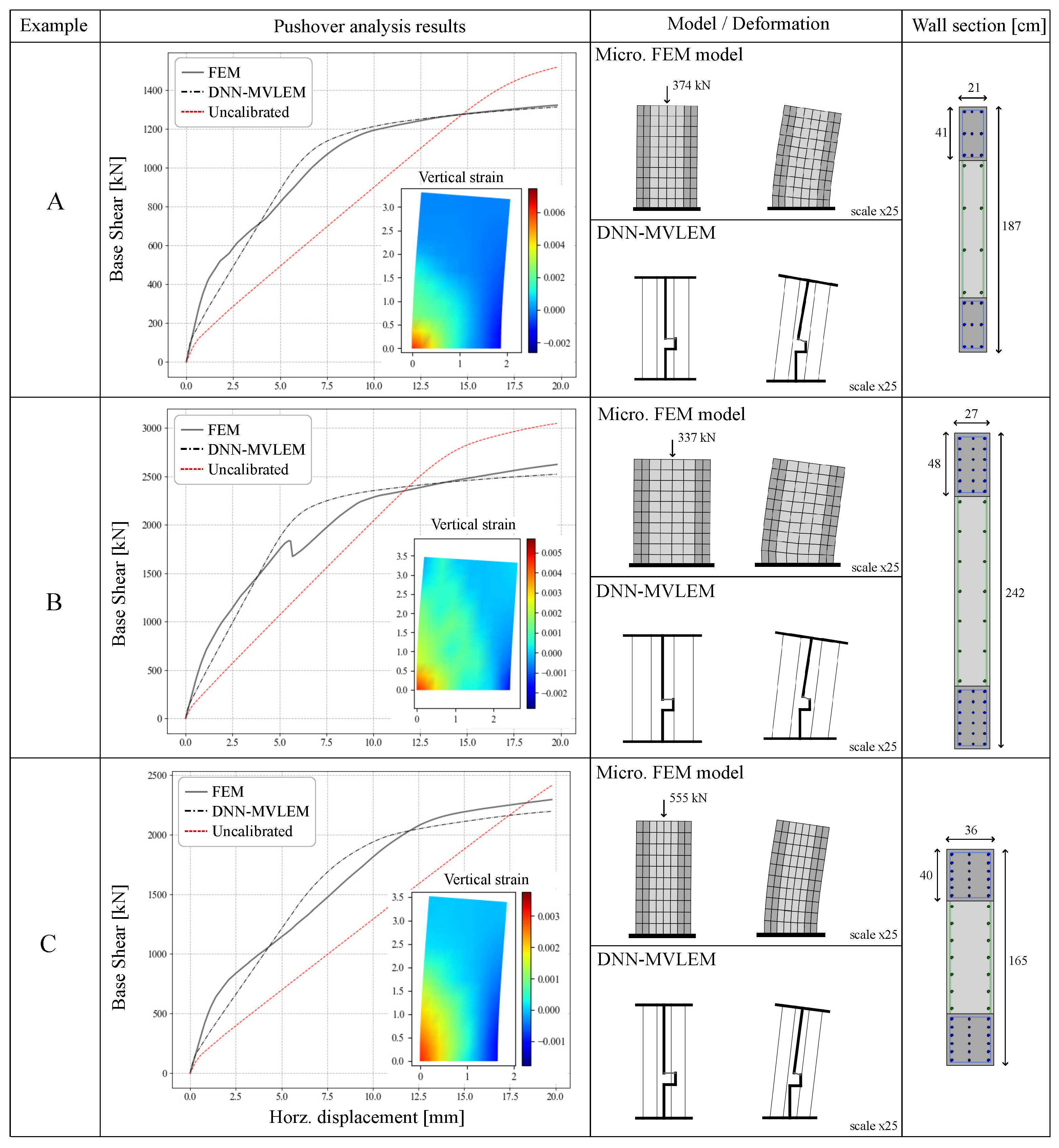
5.1. Stand-Alone RC Shear Wall

The first testing round consists of three numerical examples (A, B, C) where the wall is modeled as a stand-alone structure subjected to a static non-linear pushover analysis. The dimensions and properties for the three examples are generated randomly and correspond to the walls labeled as A, B, and C according to Table 2. The analysis is performed using both the microscopic FEM model described in Section 3, and the developed DNN-MVLEM. The boundary conditions are set so that the wall is fixed at the bottom, and a vertical load equal to $P=q_a·0.85·f_c^{\prime }·t·l_w$ is added at the top-middle node. The prescribed displacement for the pushover analysis is set to 20 mm, which is applied at a rate of 0.1 mm per step (200 total steps). The results for each example are presented and compared in Figure 10 and

Table 3. Scenario A, B, and C error and computational cost comparisons.

Scenario	Error			Computational Efficiency
	MAE [kN]	Peak Force [kN]	Total %	FEM 8 × 10 [s]	FEM 12 × 15 [s]	DNN-MVLEM [s]	Speed Factor (8 × 10)/(12 × 15)
A	37	1320	2.8	27	81	0.247	109/327
B	109	2622	4.16	36	97	0.245	146/395
C	107	2292	4.66	30	86	0.252	119/341
Averages	-	-	3.87	31	88	0.248	125/355

.

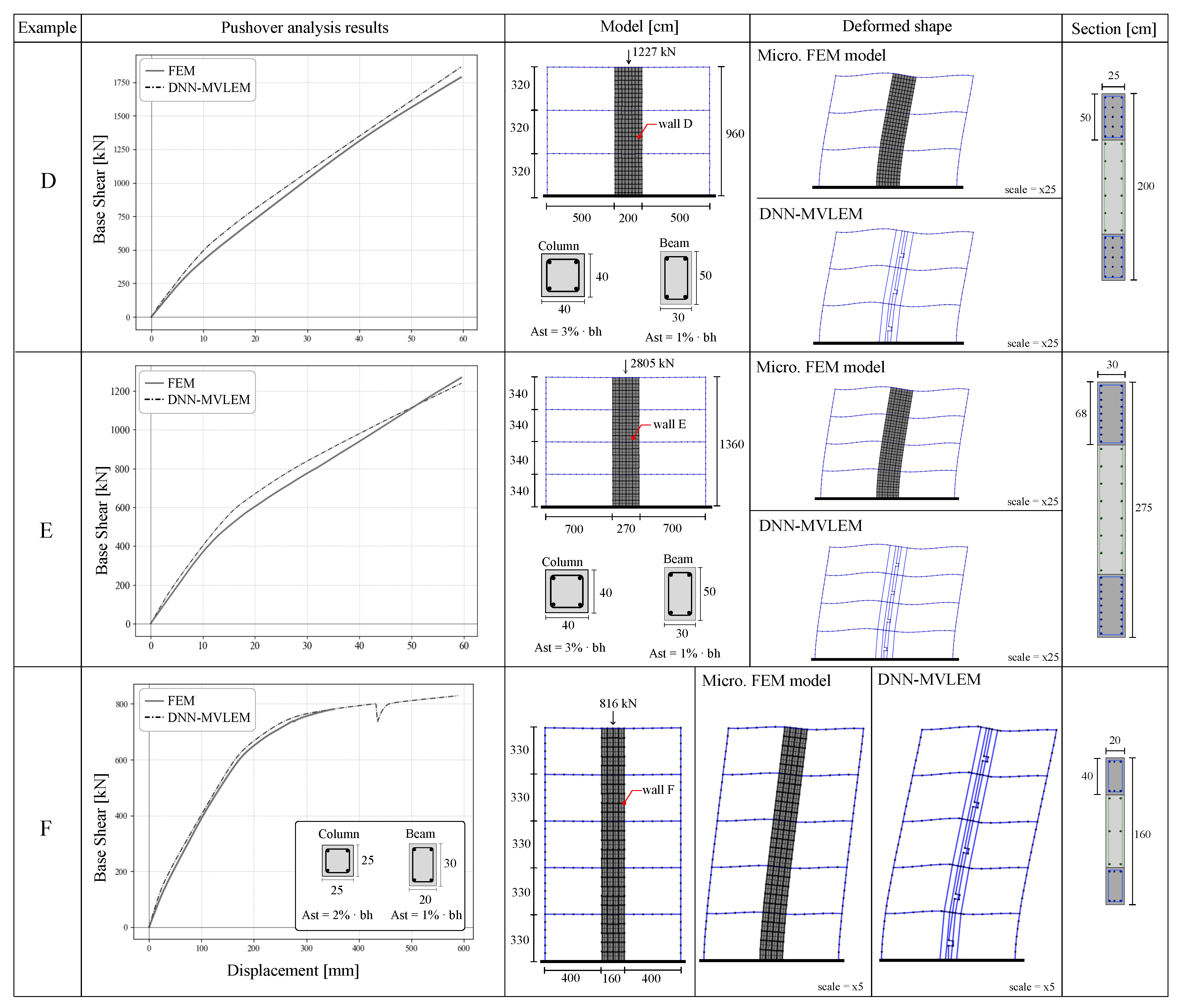
5.2. Multi-Story Frame

For the second round of tests, three additional numerical examples (D, E, F) are prepared in which the macromodel has been incorporated into a larger structure that consists of a two-bay multi-story frame. Each structure is modeled using both approaches—the microscopic FEM model and the DNN-MVLME macromodel. The additional columns and beams that form the framed structure are modeled using the same fiber section approach and the non-linear material models described in Section 2.2. For scenarios D and E, the column dimensions are set to 40 × 40 cm with $r_c=3$ cm of concrete cover and a quantity of reinforcement steel equal to $q_c=3\%$ of the concrete cross-section gross area. The beam dimensions are 30 × 50 cm with $r_c=3$ cm and $q_c=1\%$. For the third scenario F, the structure is intentionally made softer to test the methodology under extreme deformations. For such a scenario, the column dimensions are 25 × 25 cm with $r_c=2.5$ cm and $q_c=2\%$; the beam dimensions are 20 × 30 cm with $r_c=2.5$ cm and $q_c=1\%$. A static-nonlinear pushover analysis is performed for each scenario and each model. For the D and E scenarios, the prescribed displacement for the pushover analysis is 60 mm applied at a rate of 0.5 per step (120 total steps). For the third scenario, a larger target displacement of 600 mm applied at a rate of 1 mm per step is used (total 600 steps). The boundary conditions for all scenarios are set so that the bottom of the frame is fully fixed. Additionally, the vertical point load is added at the top-middle node of the top story with a magnitude equal to $P=q_a·0.85·f_c^{\prime }·t·l_w$ according to the values specified at Table 2. The results for each example are presented and compared in Figure 11 and

Table 4. Scenario D, E, and F error and computational cost comparisons.

Scenario	Error			Computational Efficiency
	MAE [kN]	Peak Force [kN]	Total %	FEM [s]	DNN-MVLEM [s]	Speed Factor
D	50	1757	2.85	82	0.979	83
E	62	1243	4.99	214	2.01	106
F	24	889	2.70	1578	10.75	146

.

6. Discussion of the Results

6.1. Accuracy

From the numerical examples, it can be appreciated that the computed pushover curve using the microscopic FEM model follows a highly non-linear path with a different shape in each case, thus illustrating the complex non-linear behavior of RC shear walls under intense lateral loading. However, despite the curves’ complex shape, the DNN-MVLEM can approximate the results with reasonable accuracy every time. The mean average error (MAE) between the pushover curve obtained with the microscopic FEM model and the one obtained with the DNN-MVLEM is computed as follows:

$$MAE=\sum _{i=1}^{nStep}\frac{|forceFE{M}_i-forceDN{N}_i|}{nStep}$$

(4)

$$e_{total}=\frac{MAE}{PeakForce}$$

(5)

where $nStep$ is the total number of steps in the pushover analysis; the term $forceFE{M}_i$ is equal to the base shear obtained with the microscopic FEM model at Step i; the term $forceDN{N}_i$ is equal to the base shear obtained with the DNN-MVLEM at the Step i; $PeakForce$ is the maximum base shear measured in the entire pushover analysis. Hence, the value $e_{total}$ is a normalization of the mean average error and provides a reasonable estimation of the overall error. With that in mind, the obtained results show that $e_{total}$ < 5% in all scenarios, which indicates a reasonably good approximation from an engineering point of view; see Table 3 and Table 4.

The accuracy referred to in this section is the approximation of the DNN-MVLEM to the reference microscopic FEM model. As it is well-known in FEM analysis, the reference FEM model is itself an approximation of the actual behavior of the structure. In Section 3.1, the accuracy of the reference FEM model is discussed.

6.2. Calibrated vs. Uncalibrated Response

In the first three scenarios, A, B, and C, the uncalibrated response of the DNN-MVLEM is also presented (i.e., the response when $k_c=K_s=K_m=1)$; see Figure 10. It can be appreciated that the calibration process is an essential step, as the uncalibrated version deviates from the actual response. Such a deviation in the uncalibrated response may be explained by the inability of the macromodel to simulate the coupled shear and flexural behavior properly, among other disparities, such as using different material models for the concrete. Nonetheless, the proposed calibration procedure using an optimization algorithm has proven to be a simple and effective solution that does not increase the complexity of the model, transferring the added computational cost to an external process to generate the database and train the DNN model.

6.3. Computational Efficiency

This study’s computational operations have been performed with a conventional PC with the following characteristics: CPU Intel Core i7-6700HQ @2.60 GHz with 16 GB RAM. These operations include creating the database, solving the calibration optimization problem using GA, training and testing the DNN, and solving the numerical examples.

The gains obtained by using the DNN-MVLEM are evident regarding the computational efficiency. For the first three scenarios, the computational cost is compared using two different mesh sizes for the microscopic FEM model, a mesh of 8 × 10 and another of 12 × 15 elements. Each pushover analysis using 200 steps takes, on average, 31 and 88 s for each case, respectively. In contrast, the DNN-MVLEM takes an average of 0.248 s. Thus, the analysis is accelerated by 125 and 355 for each case. The results are equally impressive for scenarios D, E, and F, where the speed acceleration factors obtained are 83, 106, and 146 for each case, respectively. The results are presented in Table 3 and Table 4 in the columns are labeled as “Computational Efficiency”.

On the other hand, generating the database may be a computationally expensive operation. However, the proposed microscopic FEM model based on the MLSE formulation is significantly faster than other microscopic models and poses a viable option for creating large data quantities. Each data point in the database takes approximately 1 min to be generated (30 s for the FEM analysis and 30 for the genetic algorithm). Therefore, generating the 3000 data points to train the DNN model would take about 50 h using a single PC and a single core. Nonetheless, the procedure can be significantly accelerated using parallel processing with multiple cores and computers. For example, for this study, using two computers with the same characteristics described above and running the process on multiple cores, the 3000 data points are generated in 14 h. The training of the DNN with 130,759 features takes an additional 30 s. Once the DNN is trained and ready to be used, it can be serialized into a file with a digital size of less than 5 megabytes. Loading the DNN from a file takes merely 678 milliseconds, and predicting the output for a set of input values takes less than 1 millisecond.

6.4. Advantages Summary

The advantages of the DNN-MVLEM can be summarized as follows.

• Computational Efficiency. The DNN-MVLEM can substantially speed up the non-linear analysis of large structures. In the presented numerical example labeled scenario D, a five-story frame is analyzed using both approaches. The analysis for the structure where the walls are modeled with the DNN-MVLEM is 116 times faster, taking 10.75 s to finalize compared to the 1253 s (or about 20 min) for the analysis with the walls modeled with the microscopic FEM model.
• Simplicity. The full DNN-MVLEM can be created based only on the basic properties of the RC shear wall and the pre-trained DNN model. There are no difficult-to-obtain parameters required for its definition. Furthermore, the implemented material models and element formulations are typically included in most commercial FEM packages.
• Adaptability. The methodology developed to create the DNN-MVLEM could be easily enhanced or adapted to tackle new challenges. For instance, increasing the lower and upper bound of the input values or adding additional variables to the problem. These improvements are relatively easy to implement by adding more data points to the training data and re-training the model. Similarly, the same strategy could be adapted to other types of RC shear walls, such as L-shaped or T-shaped geometries.
• Improved convergence rate. The DNN-MVLEM has been shown to have fewer convergence problems than those encountered with the microscopic FEM model. This can be appreciated in example F, where the FEM model failed to converge to the target displacement of 600 mm, but the DNN-MVLEM reached the target without issue. One potential explanation is that the elements conforming to the macromodel are based on simpler element and material formulations, making them less sensitive to convergence problems.

6.5. Scope and Applicability of DNN-MVLEM

In order to fully assess the advantages and limitations discussed in this section, it is essential to mention the objectives and motivations that led to the creation of the proposed strategy. Although the results are highly promising, DNN-MVLEM is not designed to replace traditional FEM models of RC shear walls that are grounded in well-established theoretical frameworks and have been extensively tested and verified over time. Instead, DNN-MVLEM is conceived as a more straightforward and significantly more computationally efficient alternative for certain types of analyses and problems. For example, uncertainty analysis, failure analysis, and risk assessment of structures. In these types of studies, the structure must be modeled multiple times under various conditions to determine quantities such as failure probabilities. Hence, a simpler and significantly faster model approximating the results is preferred as long as the approximation quality is good enough. For DNN-MVLEM, the obtained error for the tested examples is between 2% and 5%, which is within a reasonable range for such engineering applications.

Similarly, during the preliminary stages of a building’s design process, numerous iterations are typically needed to identify the optimal shape or layout of walls and braces to achieve the best possible performance of the building under lateral loads. Trading some accuracy for a simpler and much faster model is usually preferred at this stage. The faster model may be used for the pre-design, and once the ideal configuration has been established, the structure can be re-analyzed using a more sophisticated (and precise) model to ensure higher confidence in the final design.

6.6. Current Limitations and Future Enhancements

There are some limitations that one needs to be aware of when using DNN-MVLEM in its current form. For instance, the calibration factors slightly adjust the model’s stiffness to match the FEM results in terms of displacements. This has turned out to be a simple and straightforward solution. However, other properties of the structure, such as modal frequencies, have not been taken into account. In future versions of DNN-MVLEM, such additional quantities may be considered by including them into the optimization problem that is solved to obtain the calibration coefficients.

Another inconvenience may be encountered when defining the axial load required as input in the DNN. However, one simple solution is to perform a linear static analysis for the gravitational load case with the uncalibrated form of the macromodel (i.e., $k_c=k_s=k_m=1$), thus obtaining an estimate of the axial load, which can then be used to define the calibrated macromodel prior to the non-linear procedure.

There are also two common concerns for applying data-driven strategies in practical applications. One is the availability of the data to train the model. Nonetheless, for DNN-MVLEM that is not the case, as the data are generated using a parametric microscopic FEM model and the quantity of data is only limited by the time or computational resources, which have been discussed in Section 6.3. The second concern is the expertise that the user requires to fully comprehend and apply these methodologies. However, in this regard, big tech companies are constantly developing multiple tools that facilitate the application of machine learning techniques. Hence, nowadays, it is becoming easier to build reliable data-driven solutions.

7. Conclusions

In this study, a macromodel denoted as DNN-MVLEM has been developed for the analysis of RC shear walls. The model is created based on a novel data-driven methodology using deep neural networks. The DNN-MVLEM is composed of two main parts. The structural part, which is comprised of four vertical elements and one horizontal shear spring, and the data-driven part, which is a DNN trained to predict the properties of the shear spring and three coefficients required to calibrate the macromodel’s behavior. The data utilized to train the DNN have been generated in a two-step procedure using a microscopic FEM model based on the multi-layer shell formulation, and a genetic algorithm that determines the calibration coefficients. The DNN-MVLEM was tested in two sets of examples: as a stand-alone wall in cantilever mode and as part of a multi-story frame structure subjected to a static non-linear lateral pushover analysis. The results obtained with the DNN-MVLEM were compared to those from the microscopic FEM model, showing an estimated error of less than 5% between the two pushover curves. Moreover, the DNN-MVLEM demonstrated significantly improved computational efficiency, being up to 140 times faster than the microscopic FEM model, depending on the total number of elements in the FEM model.

This study has shown that alternative methods based on data-driven solutions are exceptionally effective in reducing the computational time of the non-linear analysis of structures with a minimum compromise in accuracy with respect to more sophisticated FEM models. In essence, the computational effort is transferred to the database creation and the DNN model’s training process. However, these heavy-duty operations can be conveniently automated using parametric modeling techniques and high-performance computing systems. Hence, significantly speeding the workflow process and enabling the practical application of such data-driven techniques. In particular, the DNN-MVLEM is suitable for applications where a large number of analysis are needed, and the engineer (or designer) is willing to sacrifice a bit of accuracy for significantly greater computational efficiency. Some examples of such applications are uncertainty analysis, failure analysis, risk assessment of structures, and optimization of buildings in preliminary design stages.

We are entering an era where artificial intelligence and data-driven solutions are becoming much more efficient and mature, thus quickly taking over traditional deterministic approaches, while the full implications of such fast phased progress is still uncertain for structural engineering, its effect is already taking place notoriously. This study serves as an example of how AI-driven techniques could revolutionize the analysis and simulation of structures in the future.

References

1. Tuna, Z. Seismic Performance, Modeling, and Failure Assessment of Reinforced Concrete Shear Wall Buildings. Ph.D. Thesis, UCLA, Los Angeles, CA, USA, 2012. [Google Scholar]
2. Fintel, M. Performance of Buildings With Shear Walls in Earthquakes of the Last Thirty Years. PCI J. 1995, 40, 62–80. [Google Scholar] [CrossRef]
3. Mo, Y.; Zhong, J.; Hsu, T. Seismic simulation of RC wall-type structures. Eng. Struct. 2008, 30, 3167–3175. [Google Scholar] [CrossRef]
4. Jalali, A.; Dashti, F. Nonlinear behavior of reinforced concrete shear walls using macroscopic and microscopic models. Eng. Struct. 2010, 32, 2959–2968. [Google Scholar] [CrossRef]
5. Mulas, M.; Coronelli, D.; Martinelli, L. Multi-scale modelling approach for the pushover analysis of existing RC shear walls—Part I: Model formulation. Earthq. Eng. Struct. Dyn. 2007, 36, 1169–1187. [Google Scholar] [CrossRef]
6. Mulas, M.; Coronelli, D.; Martinelli, L. Multi-scale modelling approach for the pushover analysis of existing RC shear walls—Part II: Experimental verification. Earthq. Eng. Struct. Dyn. 2007, 36, 1189–1207. [Google Scholar] [CrossRef]
7. Ayoub, A.; Filippou, F. Nonlinear finite-element analysis of RC shear panels and walls. J. Struct. Eng. 1998, 124, 298–308. [Google Scholar] [CrossRef]
8. Wang, J.J.; Liu, C.; Nie, X.; Fan, J.S.; Zhu, Y.J. Nonlinear model updating algorithm for biaxial reinforced concrete constitutive models of shear walls. J. Build. Eng. 2021, 44, 103215. [Google Scholar] [CrossRef]
9. Luu, C.; Mo, Y.; Hsu, T. Development of CSMM-based shell element for reinforced concrete structures. Eng. Struct. 2017, 132, 778–790. [Google Scholar] [CrossRef]
10. Liao, F.Y.; Han, L.H.; Tao, Z. Performance of reinforced concrete shear walls with steel reinforced concrete boundary columns. Eng. Struct. 2012, 44, 186–209. [Google Scholar] [CrossRef]
11. Dong, Y.R.; Xu, Z.D.; Zeng, K.; Cheng, Y.; Xu, C. Seismic behavior and cross-scale refinement model of damage evolution for RC shear walls. Eng. Struct. 2018, 167, 13–25. [Google Scholar] [CrossRef]
12. Dashti, F.; Dhakal, R.P.; Pampanin, S. Numerical Modeling of Rectangular Reinforced Concrete Structural Walls. J. Struct. Eng. 2017, 143, 04017031. [Google Scholar] [CrossRef]
13. Epackachi, S.; Whittaker, A.S. A validated numerical model for predicting the in-plane seismic response of lightly reinforced, low-aspect ratio reinforced concrete shear walls. Eng. Struct. 2018, 168, 589–611. [Google Scholar] [CrossRef]
14. El-Kashif, K.F.O.; Adly, A.K.; Abdalla, H.A. Finite element modeling of RC shear walls strengthened with CFRP subjected to cyclic loading. Alex. Eng. J. 2019, 58, 189–205. [Google Scholar] [CrossRef]
15. Kolozvari, K.; Gullu, M.F.; Orakcal, K. Finite Element Modeling of Reinforced Concrete Walls Under Uni- and Multi-Directional Loading Using Opensees. J. Earthq. Eng. 2021, 26, 6524–6547. [Google Scholar] [CrossRef]
16. Wu, Y.T.; Lan, T.Q.; Xiao, Y.; Yang, Y.B. Macro-Modeling of Reinforced Concrete Structural Walls: State-of-the-Art. J. Earthq. Eng. 2017, 21, 652–678. [Google Scholar] [CrossRef]
17. Kolozvari, K.; Arteta, C.; Fischinger, M.; Gavridou, S.; Hube, M.; Isakovic, T.; Lowes, L.; Orakcal, K.; Vásquez, G.J.; Wallace, J. Comparative Study of State-of-the-Art Macroscopic Models for Planar Reinforced Concrete Walls. ACI Struct. J. 2018, 115, 1637–1657. [Google Scholar] [CrossRef]
18. Goel, S.; Liao, W.; Bayat, M.; Chao, S. Performance-based plastic design (PBPD) method for earthquake-resistant structures: An overview. Struct. Des. Tall Spec. Build. 2010, 19, 115–137. [Google Scholar] [CrossRef]
19. Kabeyasawa, T.; Shioara, H.; Otani, S. U.S.-Japan Cooperative Research on R/C Full-Scale Building Test, Part 5: Discussion of Dynamic Response System. In Proceedings of the Eighth World Conference on Earthquake Engineering, San Francisco, CA, USA, 21–28 July 1984; Volume 6, pp. 627–634. [Google Scholar]
20. Vulcano, A.; Bertero, V.; Colotti, V. Analytical Modeling of R/C Structural Walls. In Proceedings of the 9th World Conference on Earthquake Engineering, Tokyo/Kyoto, Japan, 2–9 August 1988; Volume 6. [Google Scholar]
21. Vulcano, A. Macroscopic modeling for nonlinear analysis of RC structural walls. In Nonlinear Seismic Analysis and Design of Reinforced Concrete Buildings; CRC Press: Boca Raton, FL, USA, 1992; p. 10. [Google Scholar]
22. Orakcal, K.; Wallace, J.; Conte, J. Nonlinear modeling and analysis of slender reinforced concrete walls. ACI Struct. J. 2004, 101, 688–698. [Google Scholar]
23. Lu, X.; Chen, Y. Modeling of Coupled Shear Walls and Its Experimental Verification. J. Struct. Eng. 2005, 131, 75–84. [Google Scholar] [CrossRef]
24. Orakcal, K.; Wallace, J. Flexural modeling of reinforced concrete walls—Experimental verification. ACI Struct. J. 2006, 103, 196–206. [Google Scholar]
25. Rezapour, M.; Ghassemieh, M. Macroscopic modelling of coupled concrete shear wall. Eng. Struct. 2018, 169, 37–54. [Google Scholar] [CrossRef]
26. Isakovic, T.; Fischinger, M. Assessment of a force–displacement based multiple-vertical-line element to simulate the non-linear axial–shear–flexure interaction behaviour of reinforced concrete walls. Bull. Earthq. Eng. 2019, 17, 6369–6389. [Google Scholar] [CrossRef]
27. Kolozvari, K.; Orakcal, K.; Wallace, J.W. New opensees models for simulating nonlinear flexural and coupled shear-flexural behavior of RC walls and columns. Comput. Struct. 2018, 196, 246–262. [Google Scholar] [CrossRef]
28. Kolozvari, K.; Orakcal, K.; Wallace, J.W. Modeling of Cyclic Shear-Flexure Interaction in Reinforced Concrete Structural Walls. I: Theory. J. Struct. Eng. 2015, 141, 04014135. [Google Scholar] [CrossRef]
29. Kolozvari, K.; Tran, T.A.; Orakcal, K.; Wallace, J.W. Modeling of Cyclic Shear-Flexure Interaction in Reinforced Concrete Structural Walls. II: Experimental Validation. J. Struct. Eng. 2015, 141, 04014136. [Google Scholar] [CrossRef]
30. Zhang, H.; Fang, Y.; Duan, Y.; Du, G. The V-MVLE model for cyclic failure behavior simulation of planar RC members. Thin-Walled Struct. 2022, 181, 110159. [Google Scholar] [CrossRef]
31. Esmaeiltabar, P.; Vaseghi, J.; Khosravi, H. Nonlinear macro modeling of slender reinforced concrete shear walls. Struct. Concr. 2019, 20, 899–910. [Google Scholar] [CrossRef]
32. Fu, W. Macroscopic numerical model of reinforced concrete shear walls based on material properties. J. Intell. Manuf. 2021, 32, 1401–1410. [Google Scholar] [CrossRef]
33. Solorzano, G.; Plevris, V. Computational intelligence methods in simulation and modeling of structures: A state-of-the-art review using bibliometric maps. Front. Built Environ. 2022, 8. [Google Scholar] [CrossRef]
34. Plevris, V.; Lagaros, N.D. Artificial Intelligence (AI) Applied in Civil Engineering. Appl. Sci. 2022, 12, 7595. [Google Scholar] [CrossRef]
35. Plevris, V.; Tsiatas, G.C. Computational Structural Engineering: Past Achievements and Future Challenges. Front. Built Environ. 2018, 4, 21. [Google Scholar] [CrossRef]
36. Solorzano, G.; Plevris, V. ANN-based surrogate model for predicting the lateral load capacity of RC shear walls. In Proceedings of the ECCOMAS Congress 2022—8th European Congress on Computational Methods in Applied Sciences and Engineering, Oslo, Norway, 5–9 June 2022. [Google Scholar] [CrossRef]
37. Lagaros, N.; Papadrakakis, M. Neural network based prediction schemes of the non-linear seismic response of 3D buildings. Adv. Eng. Softw. 2012, 44, 92–115. [Google Scholar] [CrossRef]
38. Plevris, V.; Asteris, P.G. Modeling of Masonry Failure Surface under Biaxial Compressive Stress Using Neural Networks. Constr. Build. Mater. 2014, 55, 447–461. [Google Scholar] [CrossRef]
39. Moayyeri, N.; Gharehbaghi, S.; Plevris, V. Cost-Based Optimum Design of Reinforced Concrete Retaining Walls Considering Different Methods of Bearing Capacity Computation. Mathematics 2019, 7, 1232. [Google Scholar] [CrossRef]
40. Liu, J.; Xia, Y. A hybrid intelligent genetic algorithm for truss optimization based on deep neutral network. Swarm Evol. Comput. 2022, 73, 101120. [Google Scholar] [CrossRef]
41. Solorzano, G.; Plevris, V. Optimum Design of RC Footings with Genetic Algorithms According to ACI 318–319. Buildings 2020, 10, 110. [Google Scholar] [CrossRef]
42. Kallioras, N.; Kazakis, G.; Lagaros, N. Accelerated topology optimization by means of deep learning. Struct. Multidiscip. Optim. 2020, 62, 1185–1212. [Google Scholar] [CrossRef]
43. Jung, J.; Yoon, K.; Lee, P.S. Deep learned finite elements. Comput. Methods Appl. Mech. Eng. 2020, 372, 113401. [Google Scholar] [CrossRef]
44. Samaniego, E.; Anitescu, C.; Goswami, S.; Nguyen-Thanh, V.M.; Guo, H.; Hamdia, K.; Zhuang, X.; Rabczuk, T. An energy approach to the solution of partial differential equations in computational mechanics via machine learning: Concepts, implementation and applications. Comput. Methods Appl. Mech. Eng. 2020, 362, 112790. [Google Scholar] [CrossRef]
45. Kudela, J.; Matousek, R. Recent advances and applications of surrogate models for finite element method computations: A review. Soft Comput. 2022, 26, 13709–13733. [Google Scholar] [CrossRef]
46. Mai, H.T.; Kang, J.; Lee, J. A machine learning-based surrogate model for optimization of truss structures with geometrically nonlinear behavior. Finite Elem. Anal. Des. 2021, 196, 103572. [Google Scholar] [CrossRef]
47. Abueidda, D.W.; Koric, S.; Sobh, N.A. Topology optimization of 2D structures with nonlinearities using deep learning. Comput. Struct. 2020, 237, 106283. [Google Scholar] [CrossRef]
48. Linghu, J.; Dong, H.; Cui, J. Ensemble wavelet-learning approach for predicting the effective mechanical properties of concrete composite materials. Comput. Mech. 2022, 70, 335–365. [Google Scholar] [CrossRef]
49. Lee, S.; Popovics, J. Applications of physics-informed neural networks for property characterization of complex materials. Rilem Tech. Lett. 2022, 7, 178–188. [Google Scholar] [CrossRef]
50. Solorzano, G.; Plevris, V. Design of Reinforced Concrete Isolated Footings under Axial Loading with Artificial Neural Networks. In Proceedings of the 14th ECCOMAS Thematic Conference on Evolutionary and Deterministic Methods for Design, Optimization and Control (EUROGEN 2021), Athens, Greece, 28–30 June 2021; pp. 118–131. [Google Scholar] [CrossRef]
51. Ben Seghier, M.E.A.; Corriea, J.A.F.O.; Jafari-Asl, J.; Malekjafarian, A.; Plevris, V.; Trung, N.T. On the modeling of the annual corrosion rate in main cables of suspension bridges using combined soft computing model and a novel nature-inspired algorithm. Neural Comput. Appl. 2021, 33, 15969–15985. [Google Scholar] [CrossRef]
52. McKenna, F.; Scott, M.H.; Fenves, G.L. Nonlinear Finite-Element Analysis Software Architecture Using Object Composition. JOurnal Comput. Civ. Eng. 2010, 24, 95–107. [Google Scholar] [CrossRef]
53. Zhu, M.; McKenna, F.; Scott, M.H. OpenSeesPy: Python library for the OpenSees finite element framework. SoftwareX 2018, 7, 6–11. [Google Scholar] [CrossRef]
54. Taucer, F.; Spacone, E.; Filippou, F. A Fiber Beam-Column Element for Seismic Response Analysis of Reinforced Concrete Structures. Ph.D. Thesis, University of California, Berkeley, CA, USA, 1991. [Google Scholar]
55. Shah, S.P.; Swartz, S.E.; Ouyang, C. Fracture Mechanics of Concrete: Applications of Fracture Mechanics to Concrete, Rock and Other Quasi-Brittle Materials; John Wiley & Sons: Hoboken, NJ, USA, 1995. [Google Scholar]
56. Kent, D.C.; Park, R. Flexural Members with Confined Concrete. J. Struct. Div. 1971, 97, 1969–1990. [Google Scholar] [CrossRef]
57. Mander, J.B.; Priestley, M.J.N.; Park, R. Theoretical Stress-Strain Model for Confined Concrete. J. Struct. Eng. 1988, 114, 1804–1826. [Google Scholar] [CrossRef]
58. Bangash, M.Y.H. Concrete and Concrete Structures: Numerical Modelling and Applications; Elsevier Applied Science: London, UK, 1989. [Google Scholar]
59. Menegotto, M. Method of Analysis of Cyclically Loaded RC Plane Frames including Changes in Geometry and Non-Elastic Behavior of Elements under Normal Force and Bending; ETH Zürich: Zürich, Schweiz, 1973; pp. 15–22. [Google Scholar]
60. Filippou, F.C.; Popov, E.P.; Bertero, V.V. Effects of Bond Deterioration on Hysteretic Behavior of Reinforced Concrete Joints; Technical Report; Earthquake Engineering Research Center, University of California: Berkeley, CA, USA, 1983. [Google Scholar]
61. Xie, L.; Lu, X.; Lu, X.; Huang, Y.; Ye, L. Multi-Layer Shell Element for Shear Walls in OpenSees; American Society of Civil Engineers: Reston, VA, USA, 2014; pp. 1190–1197. ISBN 9780784413616. [Google Scholar] [CrossRef]
62. Lu, X.; Xie, L.; Guan, H.; Huang, Y.; Lu, X. A shear wall element for nonlinear seismic analysis of super-tall buildings using OpenSees. Finite Elem. Anal. Des. 2015, 98, 14–25. [Google Scholar] [CrossRef]
63. Guan, H.; Loo, Y.C. Flexural and Shear Failure Analysis of Reinforced Concrete Slabs and Flat Plates. Adv. Struct. Eng. 1997, 1, 71–85. [Google Scholar] [CrossRef]
64. Hallinan, P.; Guan, H. Layered Finite Element Analysis of One-Way and Two-Way Concrete Walls with Openings. Adv. Struct. Eng. 2007, 10, 55–72. [Google Scholar] [CrossRef]
65. ACI Committee 318. Building Code Requirements for Structural Concrete (ACI 318-19); ACI: Farmington Hills, MI, USA, 2019. [Google Scholar]
66. Lefas, I.; Kotsovos, M. Behavior of reinforced concrete structural walls. Strength, deformation characteristics, and failure mechanism. ACI Struct. J. 1990, 87, 23–31. [Google Scholar]
67. Lu, X.; Zhou, Y.; Yang, J.; Qian, J.; Song, C.; Wang, Y. SLDRCE Database on Static Tests of Structural Members and Joint Assemblies—Shear Walls R11; Technical Report; Institute of Structural Engineering and Disaster Reduction, Tongji University: Shanghai, China, 2008. [Google Scholar]
68. Petrone, F.; McKenna, F.; Do, T.; McCallen, D. A versatile numerical model for the nonlinear analysis of squat-to-tall reinforced-concrete shear walls. Eng. Struct. 2021, 242, 112406. [Google Scholar] [CrossRef]
69. Blank, J.; Deb, K. pymoo: Multi-Objective Optimization in Python. IEEE Access 2020, 8, 89497–89509. [Google Scholar] [CrossRef]
70. Abadi, M.; Agarwal, A.; Barham, P.; Brevdo, E.; Chen, Z.; Citro, C.; Corrado, G.S.; Davis, A.; Dean, J.; Devin, M.; et al. TensorFlow: Large-Scale Machine Learning on Heterogeneous Systems. 2015. Available online: https://www.tensorflow.org (accessed on 18 January 2022).
71. Plevris, V.; Solorzano, G.; Bakas, N.; Seghier, M.E.A. Investigation of performance metrics in regression analysis and machine learning-based prediction models. In Proceedings of the ECCOMAS Congress 2022—8th European Congress on Computational Methods in Applied Sciences and Engineering, Oslo, Norway, 5–9 June 2022. [Google Scholar] [CrossRef]
Figure 1. RC shear wall microscopic 3D FEM model using solid elements.
Mathematics 11 02347 g001
Figure 2. Popular macromodels for RC shear wall analysis. (a) Model proposed by Kabeyasawa et al. [19]. (b) The MVLEM, proposed by Vulcano et al. [20]. (c) The SFI-MVLEM proposed by Kolozvari et al. [28].
Mathematics 11 02347 g002
Figure 3. The DNN-MVLEM macromodel. (a) Main components and geometry. (b) Fiber-based discretization of the cross section used for all the vertical elements.
Mathematics 11 02347 g003
Figure 4. Illustrative uni-axial curves for the material models. (a) Concrete. (b) Reinforcement steel.
Mathematics 11 02347 g004
Figure 5. Illustrative force–displacement curve of the multi-linear model used in the shear spring obtained using an DNN.
Mathematics 11 02347 g005
Figure 6. MLSE-based microscopic FEM model. (a) Elevation and mesh. (b) Realistic cross-section. (c) MLSE discretization of the cross-section.
Mathematics 11 02347 g006
Figure 7. Comparison of the MLSE-based microscopic FEM model to experimental test results. (a) Specimen SW22 [66]. (b) Specimen SW1-1 [67].
Mathematics 11 02347 g007
Figure 8. A diagram showing the methodology that is followed to create the DNN-MVLEM.
Mathematics 11 02347 g008
Figure 9. Results of the correlation coeficients R and R 2 of the first 8 output variables for the testing set.
Mathematics 11 02347 g009
Figure 10. Comparison of results between the microscopic FEM model and the developed DNN-MVLEM for the three stand-alone analysis examples labeled A, B, and C.
Mathematics 11 02347 g010
Figure 11. Comparison of results between the microscopic FEM model and the developed DNN-MVLEM for the three multi-story frame analysis examples labeled as D, E, and F.
Mathematics 11 02347 g011