A Generalized Finite Difference Method for Solving Hamilton–Jacobi–Bellman Equations in Optimal Investment
Abstract
1. Introduction
2. Review of HJB Equation and GFDM
2.1. Review of Stochastic Optimal Control Problem and HJB Equation
2.2. Review of Generalized Finite Difference Method
3. Numerical Scheme of HJB Equations
- For the general case of the HJB equation coupled with optimization, we propose a successive approximation algorithm which combines the GFDM discretization scheme with the optimization algorithm.
- For the special case where one can explicitly express the optimal control u by maximizing the Hamiltonian, we propose an algorithm combining the GFDM and Newton’s iterative method.
3.1. The General Case
Algorithm 1 Successive Approximation Algorithm |
| Input: Initial control law ; given tolerance Output: Approximation of control law , value function
|
3.2. The Special Case
Algorithm 2 Newton Iterations |
Input: Initial guess ; max number of iterations ; given tolerance Output: Approximation of Initialize ; while do Compute and based on each discrete equation Let solve: if then break end if end while return |
4. Case Study
4.1. Optimal Investment Problem
4.2. Numerical Results
4.2.1. The Regular Node Distributions
4.2.2. The Irregular Node Distributions
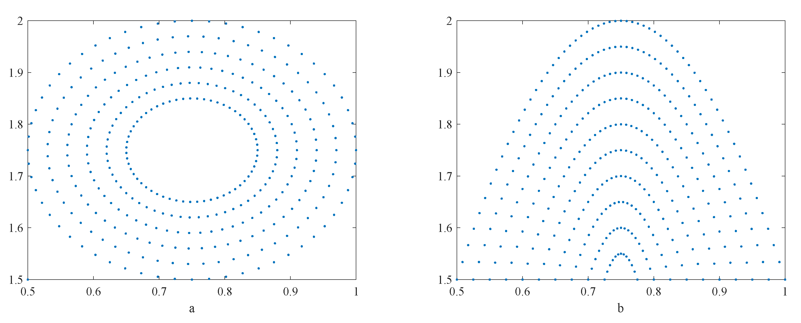
- Shape a:
- Shape b: .
5. Conclusions
Author Contributions
Funding
Data Availability Statement
Conflicts of Interest
References
- Merton, R.C. Analytical optimal control theory as applied to stochastic and non-stochastic economics. Doctoral Dissertation, Massachusetts Institute of Technology, Cambridge, MA, USA, 1970. [Google Scholar]
- Abel, A.B. Optimal investment under uncertainty. Am. Econ. Rev. 1983, 73, 228–233. [Google Scholar]
- Karatzas, I. Optimization problems in the theory of continuous trading. SIAM J. Control Optim. 1989, 27, 1221–1259. [Google Scholar] [CrossRef]
- Dixit, A.K.; Pindyck, R.S. Investment under Uncertainty; Princeton University Press: Princeton, NJ, USA, 1994. [Google Scholar]
- Zhou, X.Y.; Li, D. Continuous-time mean-variance portfolio selection: A stochastic LQ framework. Appl. Math. Optim. 2000, 42, 19–33. [Google Scholar] [CrossRef]
- Bellman, R. The theory of dynamic programming. Bull. Am. Math. Soc. 1954, 60, 503–515. [Google Scholar] [CrossRef]
- Ji, S.; Zhou, X.Y. A maximum principle for stochastic optimal control with terminal state constraints, and its applications. Commun. Inf. Syst. 2006, 6, 321–337. [Google Scholar] [CrossRef]
- Peng, S. A general stochastic maximum principle for optimal control problems. SIAM J. Control Optim. 1990, 28, 966–979. [Google Scholar] [CrossRef]
- Zhou, X.Y. A unified treatment of maximum principle and dynamic programming in stochastic controls. Stoch. Rep. 1991, 36, 137–161. [Google Scholar]
- Ma, K.; Forsyth, P.A. Numerical solution of the Hamilton–Jacobi-Bellman formulation for continuous-time mean-variance asset allocation under stochastic volatility. J. Comput. Financ. 2016, 20, 1–37. [Google Scholar] [CrossRef]
- Naicker, V.; Andriopoulos, K.; Leach, P.G.L. Symmetry reductions of a Hamilton–Jacobi- Bellman equation arising in financial mathematics. J. Nonlinear Math. Phys. 2005, 12, 268–283. [Google Scholar] [CrossRef]
- Wang, J.; Forsyth, P.A. Numerical solution of the Hamilton–Jacobi-Bellman formulation for continuous time mean variance asset allocation. J. Econ. Dyn. Control 2010, 34, 207–230. [Google Scholar] [CrossRef]
- Wang, S.; Gao, F.; Teo, K.L. An upwind finite-difference method for the approximation of viscosity solutions to Hamilton–Jacobi-Bellman equations. IMA J. Math. Control Inf. 2000, 17, 167–178. [Google Scholar] [CrossRef]
- Peyrl, H.; Herzog, F.; Geering, H.P. Numerical solution of the Hamilton–Jacobi-Bellman equation for stochastic optimal control problems. In Proceedings of the 2005 WSEAS International Conference on Dynamical Systems and Control, VCE, Venice, Italy, 2–4 November 2005; pp. 489–497. [Google Scholar]
- Ma, J.; Ma, J. Finite difference methods for the Hamilton–Jacobi-Bellman equations arising in regime switching utility maximization. J. Sci. Comput. 2020, 85, 1–27. [Google Scholar] [CrossRef]
- Inoue, D.; Ito, Y.; Kashiwabara, T.; Saito, N.; Yoshida, H. Convergence Analysis of the Upwind Difference Methods for Hamilton–Jacobi-Bellman Equations. arXiv 2023, arXiv:2301.06415. [Google Scholar]
- Forsyth, P.A.; Labahn, G. Numerical methods for controlled Hamilton–Jacobi-Bellman PDEs in finance. J. Comput. Financ. 2007, 11, 1–44. [Google Scholar] [CrossRef]
- Boulbrachene, M.; Haiour, M. The finite element approximation of Hamilton–Jacobi-Bellman equations. Comput. Math. Appl. 2001, 41, 993–1007. [Google Scholar] [CrossRef]
- Jensen, M.; Smears, I. On the convergence of finite element methods for Hamilton–Jacobi –Bellman equations. SIAM J. Numer. Anal. 2013, 51, 137–162. [Google Scholar] [CrossRef]
- Jaroszkowski, B.; Jensen, M. Finite Element Approximation of Hamilton–Jacobi-Bellman equations with nonlinear mixed boundary conditions. arXiv 2021, arXiv:2105.09585. [Google Scholar] [CrossRef]
- Smears, I. Hamilton-Jacobi-Bellman Equations, Analysis and Numerical Analysis. Univ. Durham, Durham, UK. Available online: http://fourier.dur.ac.uk/Ug/projects/highlights/PR4/SmearsHJBreport.pdf (accessed on 2 February 2018).
- Wu, S. C0 finite element approximations of linear elliptic equations in non-divergence form and Hamilton–Jacobi-Bellman equations with Cordes coefficients. Calcolo 2021, 58, 1–26. [Google Scholar] [CrossRef]
- Mousavi, A.; Lakkis, O.; Mokhtari, R. A least-squares Galerkin approach to gradient recovery for Hamilton–Jacobi-Bellman equation with Cordes coefficients. arXiv 2022, arXiv:205.07583. [Google Scholar]
- Dleuna Nyoumbi, C.; Tambue, A. A fitted finite volume method for stochastic optimal control problems in finance. AIMS Math. 2021, 6, 3053–3079. [Google Scholar] [CrossRef]
- Gooran Orimi, A.; Effati, S.; Farahi, M.H. Approximate solution of the Hamilton–Jacobi-Bellman equation. J. Math. Model. 2022, 10, 71–91. [Google Scholar]
- Richardson, S.; Wang, S. Numerical solution of Hamilton–Jacobi-Bellman equations by an exponentially fitted finite volume method. Optimization 2006, 55, 121–140. [Google Scholar]
- Cui, L.J.; Lin, C.D. Lattice-Gas-Automaton Modeling of Income Distribution. Entropy 2020, 22, 778. [Google Scholar] [CrossRef] [PubMed]
- Scheidegger, S.; Bilionis, I. Machine learning for high-dimensional dynamic stochastic economies. J. Comput. Sci. 2019, 33, 68–82. [Google Scholar] [CrossRef]
- Song, H.M.; Qi, Z.R. A fast numerical method for the valuation of American lookback put options. Newsl. Nonlinear Sci. Numer. Simul. 2015, 27, 302–313. [Google Scholar] [CrossRef]
- Song, H.M.; Wang, X.S.; Zhang, K.; Zhang, Q. Primal-Dual Active Set Method for American Lookback Put Option Pricing. East Asian J. Appl. Math. 2017, 7, 603–614. [Google Scholar] [CrossRef]
- Zhang, Q.; Song, H.M.; Yang, C.B.; Wu, F.F. An efficient numerical method for the valuation of American multi-asset options. J. Comput. Appl. Math. 2020, 39, 1–12. [Google Scholar] [CrossRef]
- De Angelis, T.; Ferrari, G.; Martyr, R.; Moriarty, J. Optimal entry to an irreversible investment plan with non convex costs. Math. Financ. Econ. 2017, 11, 423–454. [Google Scholar] [CrossRef]
- Lagaris, I.E.; Likas, A.C.; Papageorgiou, D.G. Neural-network methods for boundary value problems with irregular boundaries. IEEE Trans. Neural Netw. 2000, 11, 1041–1049. [Google Scholar] [CrossRef]
- Huang, C.S.; Wang, S.; Chen, C.S. A radial basis collocation method for Hamilton–Jacobi-Bellman equation. Automatica 2006, 42, 2201–2207. [Google Scholar] [CrossRef]
- Alwardi, H.; Wang, S.; Richardon, S. An adaptive least-squares collocation radial basis function method for the HJB equation. J. Glob. Optim. 2012, 52, 305–322. [Google Scholar] [CrossRef]
- Swaidan, W.; Hussin, A. Feedback control method using Haar wavelet operational matrices for solving optimal control problems. Abstr. Appl. Anal. 2013, 2013, 240352. [Google Scholar] [CrossRef]
- Mehrali-Varjani, M.; Shamsi, M.; Malek, A. Solving a class of Hamilton–Jacobi-Bellman equations using pseudospectral methods. Kybernetika 2018, 54, 629–647. [Google Scholar] [CrossRef]
- Benito, J.J.; Ureña, F.; Gavete, L. Influence of several factors in the generalized finite difference method. Appl. Math. Model. 2001, 25, 1039–1053. [Google Scholar] [CrossRef]
- Gavete, L.; Ureña, F.; Benito, J.J.; García, A.; Ureña, M.; Salete, E. Solving second order non-linear elliptic partial differential equations using generalized finite difference method. J. Comput. Appl. Math. 2017, 318, 378–387. [Google Scholar] [CrossRef]
- Benito, J.J.; Ureña, F.; Gavete, L. Solving parabolic and hyperbolic equations by the generalized finite difference method. J. Comput. Appl. Math. 2007, 209, 208–233. [Google Scholar] [CrossRef]
- Ureña, F.; Gavete, L.; García, A.; Benito, J.J.; Vargas, A.M. Solving second order non-linear parabolic PDEs using generalized finite difference method (GFDM). J. Comput. Appl. Math. 2019, 354, 221–241. [Google Scholar] [CrossRef]
- Kloeden, P.E.; Platen, E. Stochastic Differential Equations; Springer: Berlin/Heidelberg, Germany, 1992. [Google Scholar]
- Gavete, L.; Benito, J.J.; Ureña, F. Generalized finite differences for solving 3D elliptic and parabolic equations. Appl. Math. Model. 2016, 40, 955–965. [Google Scholar] [CrossRef]
- Smith, G.D.; Smith, G.D.; Smith, G.D.S. Numerical Solution of Partial Differential Equations: Finite Difference Methods; Oxford University Press: New York, NY, USA, 1985. [Google Scholar]
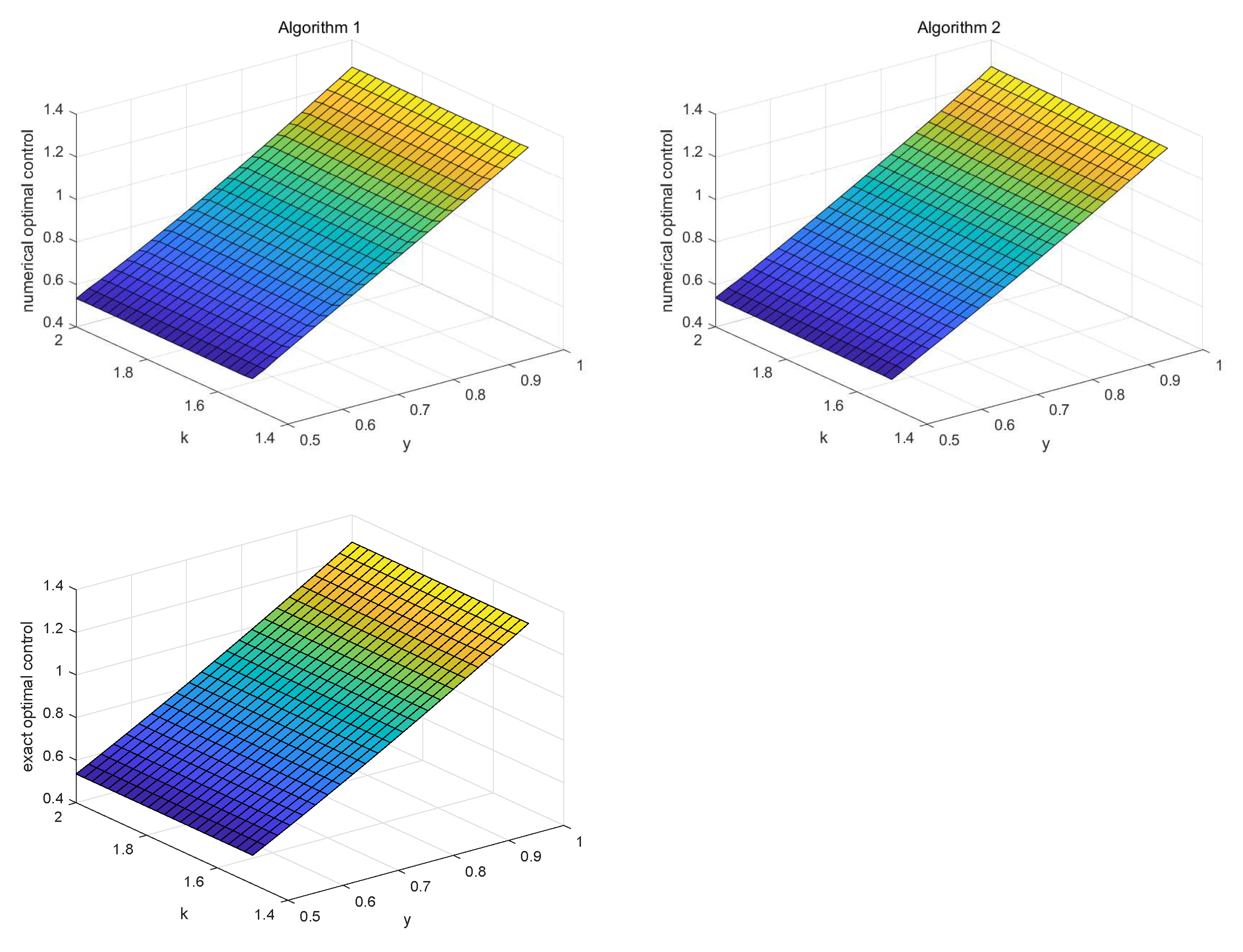


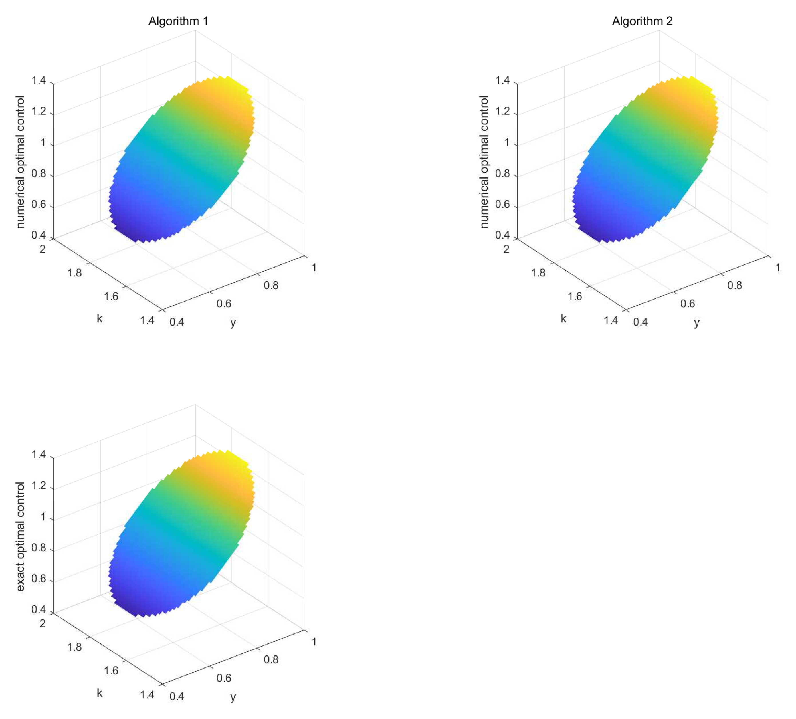


| N | Algorithm | Global Error (V) | mre (V) | Global Error (u) | mre (u) |
|---|---|---|---|---|---|
| 64 | 1 | 2.0781 × 10 | 2.9544 × 10 | 5.6422 × 10 | 4.0917 × 10 |
| 2 | 1.8414 × 10 | 4.0311 × 10 | 4.7054 × 10 | 3.4200 × 10 | |
| 225 | 1 | 1.9742 × 10 | 2.5480 × 10 | 4.9443 × 10 | 2.5629 × 10 |
| 2 | 1.0119 × 10 | 1.4615 × 10 | 1.1014 × 10 | 7.8821 × 10 | |
| 361 | 1 | 1.2136 × 10 | 1.5951 × 10 | 3.4399 × 10 | 1.5857 × 10 |
| 2 | 7.1307 × 10 | 1.2235 × 10 | 6.0667 × 10 | 7.0508 × 10 | |
| 529 | 1 | 8.2071 × 10 | 1.0909 × 10 | 2.5735 × 10 | 1.0818 × 10 |
| 2 | 2.6321 × 10 | 4.7869 × 10 | 4.0350 × 10 | 2.6199 × 10 |
| N | Algorithm 1 | Algorithm 2 | |||||
|---|---|---|---|---|---|---|---|
| Time (s) | Time (s) | ||||||
| 64 | 1/14 | 1.1794 × 10 | 1.906 | 0.46 | 5.4618 × 10 | 1.703 | 0.32 |
| 225 | 1/28 | 3.1493 × 10 | 1.905 | 1.86 | 1.7476 × 10 | 1.644 | 1.10 |
| 361 | 1/36 | 1.9458 × 10 | 1.916 | 3.09 | 1.0931 × 10 | 1.867 | 1.57 |
| 529 | 1/44 | 1.3199 × 10 | 1.934 | 4.36 | 7.4195 × 10 | 1.931 | 2.73 |
| N | Algorithm | Global Error (V) | mre (V) | Global Error (u) | mre (u) |
|---|---|---|---|---|---|
| 64 | GFDM | 2.0781 × 10 | 2.9544 × 10 | 5.6422 × 10 | 4.0917 × 10 |
| FDM | 2.1321 × 10 | 4.4319 × 10 | 7.1449 × 10 | 9.1369 × 10 | |
| 225 | GFDM | 1.9742 × 10 | 2.5480 × 10 | 4.9443 × 10 | 2.5629 × 10 |
| FDM | 2.0754 × 10 | 3.0998 × 10 | 5.1921 × 10 | 6.3504 × 10 | |
| 361 | GFDM | 1.2136 × 10 | 1.5951 × 10 | 3.4399 × 10 | 1.5857 × 10 |
| FDM | 1.8986 × 10 | 2.4111 × 10 | 4.1956 × 10 | 5.2431 × 10 | |
| 529 | GFDM | 8.2071 × 10 | 1.0909 × 10 | 2.5735 × 10 | 1.0818 × 10 |
| FDM | 9.5459 × 10 | 1.2736 × 10 | 3.7906 × 10 | 4.5419 × 10 |
| N | Weighting Functions | Global Error (V) | mre (V) | Global Error (u) | mre (u) |
|---|---|---|---|---|---|
| 2.0816 × 10 | 2.9594 × 10 | 5.6588 × 10 | 4.1064 × 10 | ||
| 2.0746 × 10 | 2.9494 × 10 | 5.6256 × 10 | 4.0771 × 10 | ||
| 64 | 1.8371 × 10 | 2.6113 × 10 | 4.7302 × 10 | 3.3365 × 10 | |
| 1.5793 × 10 | 2.2421 × 10 | 3.8283 × 10 | 2.6050 × 10 | ||
| 1.9751 × 10 | 2.5492 × 10 | 4.9469 × 10 | 2.5643 × 10 | ||
| 1.9732 × 10 | 2.5468 × 10 | 4.9419 × 10 | 2.5614 × 10 | ||
| 225 | 9.9952 × 10 | 1.1013 × 10 | 2.4839 × 10 | 1.1695 × 10 | |
| 1.4409 × 10 | 1.8664 × 10 | 3.6017 × 10 | 1.8337 × 10 | ||
| 1.2139 × 10 | 1.5955 × 10 | 3.4409 × 10 | 1.5862 × 10 | ||
| 1.2132 × 10 | 1.5946 × 10 | 3.4389 × 10 | 1.5851 × 10 | ||
| 361 | 1.0514 × 10 | 1.3844 × 10 | 2.9795 × 10 | 1.3648 × 10 | |
| 8.8539 × 10 | 1.1680 × 10 | 2.5104 × 10 | 1.1440 × 10 | ||
| 8.2087 × 10 | 1.0911 × 10 | 2.5740 × 10 | 1.0820 × 10 | ||
| 8.2055 × 10 | 1.0907 × 10 | 2.5730 × 10 | 1.0815 × 10 | ||
| 529 | 7.1091 × 10 | 9.4666 × 10 | 2.2295 × 10 | 9.3215 × 10 | |
| 5.9865 × 10 | 7.9877 × 10 | 1.8787 × 10 | 7.8164 × 10 |
| Shape | Algorithm | Global Error (V) | mre (V) | Global Error (u) | mre (u) |
|---|---|---|---|---|---|
| a | 1 | 1.4845 × 10 | 1.6205 × 10 | 2.3411 × 10 | 1.7330 × 10 |
| 2 | 1.7672 × 10 | 2.0889 × 10 | 7.7989 × 10 | 7.8551 × 10 | |
| b | 1 | 4.6104 × 10 | 4.6373 × 10 | 4.5303 × 10 | 4.0952 × 10 |
| 2 | 8.0699 × 10 | 1.0453 × 10 | 1.5865 × 10 | 1.0809 × 10 |
| Shape | IIC | Global Error (V) | mre (V) | Global Error (u) | mre (u) |
|---|---|---|---|---|---|
| a | 2.4362 × 10 | 1.8241 × 10 | 3.1043 × 10 | 1.6932 × 10 | 1.8460 × 10 |
| b | 2.1311 × 10 | 8.0699 × 10 | 1.0453 × 10 | 1.5865 × 10 | 1.0809 × 10 |
| Shape | Weighting Functions | n | Global Error (V) | mre (V) | Global Error (u) | mre (u) |
|---|---|---|---|---|---|---|
| 0.5 | 1.7631 × 10 | 2.0844 × 10 | 7.7985 × 10 | 7.8864 × 10 | ||
| 1 | 1.7672 × 10 | 2.0889 × 10 | 7.7989 × 10 | 7.8551 × 10 | ||
| a | 1.5 | 1.7718 × 10 | 2.0936 × 10 | 7.7993 × 10 | 7.8838 × 10 | |
| 0.5 | 2.5221 × 10 | 2.3074 × 10 | 7.4626 × 10 | 7.2931 × 10 | ||
| 1 | 1.8287 × 10 | 1.6347 × 10 | 7.3280 × 10 | 7.1948 × 10 | ||
| 1.5 | 1.3395 × 10 | 1.4910 × 10 | 7.3636 × 10 | 7.5369 × 10 | ||
| 0.5 | 8.0773 × 10 | 1.0463 × 10 | 1.5875 × 10 | 1.0816 × 10 | ||
| 1 | 8.0699 × 10 | 1.0453 × 10 | 1.5865 × 10 | 1.0809 × 10 | ||
| b | 1.5 | 8.0625 × 10 | 1.0443 × 10 | 1.5855 × 10 | 1.0801 × 10 | |
| 0.5 | 5.7602 × 10 | 7.7763 × 10 | 1.4208 × 10 | 8.9286 × 10 | ||
| 1 | 1.3814 × 10 | 9.3381 × 10 | 3.4880 × 10 | 1.5311 × 10 | ||
| 1.5 | 4.9254 × 10 | 5.8692 × 10 | 1.7206 × 10 | 1.0926 × 10 |
Disclaimer/Publisher’s Note: The statements, opinions and data contained in all publications are solely those of the individual author(s) and contributor(s) and not of MDPI and/or the editor(s). MDPI and/or the editor(s) disclaim responsibility for any injury to people or property resulting from any ideas, methods, instructions or products referred to in the content. |
© 2023 by the authors. Licensee MDPI, Basel, Switzerland. This article is an open access article distributed under the terms and conditions of the Creative Commons Attribution (CC BY) license (https://creativecommons.org/licenses/by/4.0/).
Share and Cite
Lin, J.; Li, X.; Hoe, S.; Yan, Z. A Generalized Finite Difference Method for Solving Hamilton–Jacobi–Bellman Equations in Optimal Investment. Mathematics 2023, 11, 2346. https://doi.org/10.3390/math11102346
Lin J, Li X, Hoe S, Yan Z. A Generalized Finite Difference Method for Solving Hamilton–Jacobi–Bellman Equations in Optimal Investment. Mathematics. 2023; 11(10):2346. https://doi.org/10.3390/math11102346
Chicago/Turabian StyleLin, Jiamian, Xi Li, SingRu (Celine) Hoe, and Zhongfeng Yan. 2023. "A Generalized Finite Difference Method for Solving Hamilton–Jacobi–Bellman Equations in Optimal Investment" Mathematics 11, no. 10: 2346. https://doi.org/10.3390/math11102346
APA StyleLin, J., Li, X., Hoe, S., & Yan, Z. (2023). A Generalized Finite Difference Method for Solving Hamilton–Jacobi–Bellman Equations in Optimal Investment. Mathematics, 11(10), 2346. https://doi.org/10.3390/math11102346


