Review

Mathematical Models in High-Temperature Viscometry: A Review

Institute of Engineering and Technology, South Ural State University, Lenin Ave, 76, 454080 Chelyabinsk, Russia
Mathematics 2023, 11(10), 2300; https://doi.org/10.3390/math11102300
Submission received: 10 April 2023 / Revised: 9 May 2023 / Accepted: 10 May 2023 / Published: 15 May 2023

Abstract

:
We systematize and review the mathematical models for use in oscillating-cup viscometry to solve different problems: for analysis of fluid flow and viscometer oscillations, for estimation of rheological constants and density, and for study without taking into account the traditional assumptions of this method. The full model for the cup and bob viscometer and a model for the oscillating-plate viscometer are also considered.

1. Introduction

The oscillating-cup viscometer has been the dominant technique for high-temperature melts (liquid crystals, molten metals and alloys, semiconductors, salts, etc.) since the middle of the 20th century up to the present day. These devices are constructed by researchers for measurements in both engineering (nuclear energetics, metallurgical industry) and physics (e.g., [1,2,3,4,5,6,7,8,9,10,11,12]). The advantages of this technique are related to high melting points, chemical activity, and low melt viscosity. These advantages include design simplicity, ease of use in an inert atmosphere with inactive materials, absence of an immersion probe, precise measurement of oscillation parameters, absolute technique, and small specimen volumes, i.e., isothermality, among others.
Traditionally, the mathematical model for the viscometer is built with some assumptions. The method can be used beyond them, and not taking them into account can lead to measurement errors. Viscometric data on metal melts contain enough contradictions (e.g., the review in [13]), and the question of their reasons is a principal one for condensed matter physics. Experimental uncertainty and error analysis are the main problems for this method [14,15,16]. Furthermore, the study of the non-Newtonian behavior of metal melts is actively discussed in experiments with serially produced rotational viscometers [17,18]. However, they are not mainly suitable for high-temperature studies, and discrepancies in the data of different authors can reach three orders of magnitude for the same melts and shear rates [19,20]. These discrepancies are also observed for the oscillating-cup method that is traditionally used for Newtonian fluids. The theory needs revision to find the sources of these discrepancies, develop an effective mathematical model, and analyze its assumptions.
The oscillating-cup viscometer is a right circular cylinder (1) filled with a fluid (2) and suspended from a thin torsion member (3), so it performs oscillations about the vertical axis (Figure 1). The viscometer usually works in damped mode. In this paper, we discuss this mode by default, and the forced mode is considered a specific case. Schematic views or photos of a viscometer are given, e.g., in [21,22,23,24,25,26].
The main experimental parameters are the following: (i) the fluid properties: density ρ and rheological constants, e.g., the kinematic viscosity ν for Newtonian fluids; (ii) the viscometer parameters: the natural period τ 0 and the decrement δ 0 of oscillations for the fluid mass M = 0 , the inertia moment K of the empty viscometer with respect to its axis; the geometric characteristics: the height H and the radius R of the fluid sample; (iii) the parameters of oscillations, e.g., the logarithmic decrement δ and the period τ of the steady linear oscillations in the damped mode.
These parameters give three dimensionless groups: A = 0.5 M R 2 / K , ξ 0 = R / d , and χ = H / R , where the boundary-layer thickness is d = v / θ , with θ being the angular frequency. The period τ > τ 0 and decrement δ > δ 0 are due to a larger effective moment of inertia and extra dissipation of mechanical energy in the presence of viscous friction, respectively.
In the general case, the model for the oscillating-cup experiments includes the partial differential equations for the fluid flow: the momentum conservation equation, the mass conservation equation and the rheological constitutive equation, and the coupled nonlinear equation of the cup oscillations. We give the simplified models obtained from the general model by using the different assumptions and systematize the solutions and applications of the results obtained from them. We review both the classical problems and the working equations for linear fluids (viscous and viscoelastic) and the novel trends in oscillating-cup viscometry for nonlinear fluids, for higher amplitudes of oscillations, etc.
The models are used in the direct and inverse problems of viscometry to study fluid properties and to model the oscillation law, respectively. The last one includes an analysis of the features for the flow and cup oscillations, an experimental design, and parameter identification in experiments with metal melts.

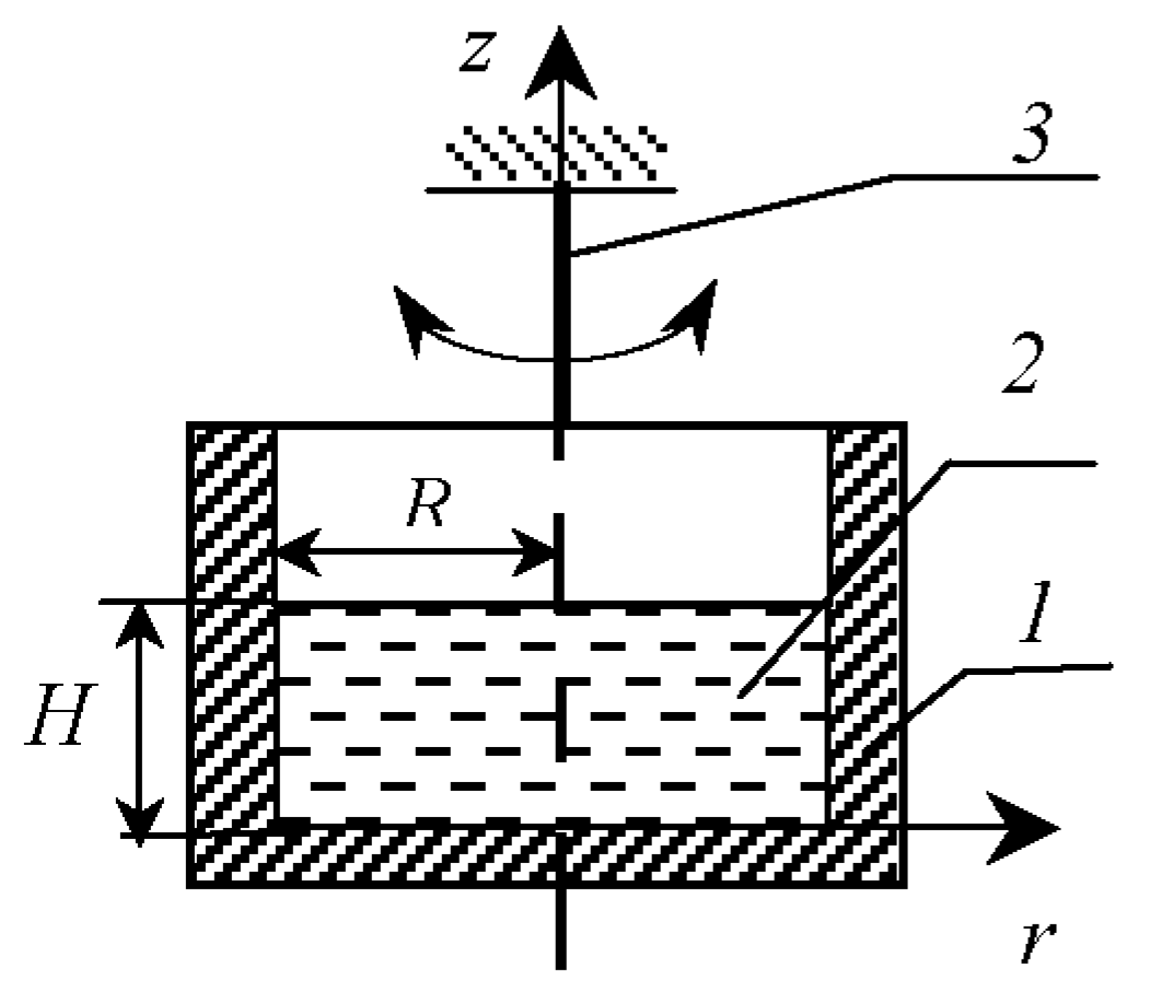
2. Full Axisymmetric Case

We take the case of an axially symmetric fluid flow in the oscillating-cup viscometer. The mass and momentum conservation equations have the form
ϑ r r + ϑ r r + ϑ z z = 0 ,
ρ ( ϑ r t + ϑ r ϑ r r + ϑ z ϑ r z ϑ ϕ 2 r ) = p r + σ r r r + σ r z z + σ r r σ ϕ ϕ r ,
ρ ( ϑ ϕ t + ϑ r ϑ ϕ r + ϑ z ϑ ϕ z + ϑ r ϑ ϕ r ) = σ ϕ r r + σ ϕ z z + 2 σ ϕ r r ,
ρ ( ϑ z t + ϑ r ϑ z r + ϑ z ϑ z z ) = p z ρ g + σ r z r + σ z z z + σ r z r .
For oscillations of the cylinder, we have the equation
α ¨ = P Σ / K ,
where P Σ = P + P 0 + P f and P = 2 π R 3 0 H σ ϕ r | R d z + 2 π 0 R ( σ ϕ z | 0 ( ( a 1 ) σ ϕ z | H ) ) r 2 d r , and for the linear case of the suspension stiffness, P 0 = 2 δ 0 α ˙ / τ 0 + N α / K .
In Equations (1)–(5), a is the number of viscometer end walls ( a = 1 for a fluid with a free surface at z = H and a = 2 for a full cylinder with a lid); α is the angular displacement of the cylinder from equilibrium; N is the stiffness coefficient of the suspended wire; ϑ r , ϑ ϕ , and ϑ z are the radial, azimuthal, and axial components of the velocity vector; g is the free-fall acceleration; p is the pressure; P Σ is the total torque of external forces acting on the viscometer about the rotation axis; P is the torque exerted by a fluid; P 0 = P e + P r is the torque acting also on the empty cup system; P e is the elastic torque of the suspension torsion; P r is the resistance torque (due to the resistance in the surrounding air and the internal friction of the suspension wire); P f is the varying external action, e.g., P f = F sin ω t ; F and ω are the amplitude and the angular frequency of the driving torque, respectively; for the damped oscillations, P f = 0 ; r , z , and φ are the radial, axial, and angular coordinates ( r = 0 on the cylinder axis and z = 0 on the bottom); σ i j is the i j -th component of the extra-stress tensor σ ; t is the time; ρ = const ; in the forced mode, the natural frequency ω 0 of the system is found from the resonance frequency and amplitude at M = 0 ; the overdot denotes the time derivative.
The model includes the initial and no-slip boundary conditions:
t = 0 : ϑ r = ϑ z = ϑ ϕ = 0 ;   ( i )   α = α 0 ~ 6 ,   d α / d T = 0 ,   ( ii )   α = 0 ,   d α / d T 0   ( ~ α 0 ) ,   ( iii )   t ( 0 , t 0 ) :   P f 0   for   ( i )   or   ( ii ) ,   t t 0 :   P f = 0 ; r = 0 :   ϑ r = ϑ ϕ = d ϑ z / r = 0 ;   r = R :   ϑ r = ϑ z = 0 ,   ϑ ϕ = α ˙ R ;   z = 0 :   ϑ r = ϑ z = 0 ,   ϑ ϕ = α ˙ r ;
z = H :   ϑ r = ϑ z = 0 ,   ϑ ϕ = α ˙ r   ( a = 2 ) ,   and   ϑ r / z = ϑ ϕ / z = ϑ z = 0   ( a = 1 ) .
The equation set is supplemented with the rheological constitutive equation for the Newtonian, Bingham, and upper-convected Maxwell models [27], respectively:
σ = 2 ν ρ D ,
σ = ( 2 ν ρ + σ 0 / I I D ) D for I I σ σ 0 ;   D = 0 for I I σ < σ 0 ,
σ + λ σ = 2 ν ρ D
where D is the tensor of the deformation rates; I I A = ( A i j A i j / 2 ) 1 / 2 is the second invariant of a tensor A ; A i j is the i j -th component of A ; λ is the relaxation time; ν is the kinematic viscosity after yielding; σ 0 is the yield stress.
The model is applied to analyze the secondary flows, the oscillations with higher amplitudes, and the features of the case without taking into account the traditional assumptions of the oscillating-cup method in the general case [1,28,29,30,31,32,33].

3. Traditional Assumptions

3.1. Mathematical Model

The traditional assumptions of the oscillating-cup method [1,34] are as follows: the fluid is incompressible, the wall slip is absent, and the oscillation amplitudes are small. In addition, the fluid flow is axisymmetric, the substantial velocity component is ϑ φ , the convective terms in (2)–(4) are absent, and the model (1)–(6) has the following form:
d 2 α d T 2 + δ 0 π d α d T + ( 1 + δ 0 2 4 π 2 ) α = P ,  
U T = σ ξ ϕ ξ + 2 σ ξ ϕ ξ + σ η ϕ η ,  
T = 0 : α ~ 6 ,   d α d T = 0 ,   U = 0 ;   ξ = ξ 0 :   U = d α d T ξ 0 ; ξ = 0 :   U = 0 ;   η = 0 ,   η = 2 η 0   ( a = 2 )   or   η = η 0   ( a = 1 ) :   U = d α d T ξ ,
with the rheological equation for Newtonian fluids
σ ξ ϕ ( η ϕ ) = D ξ ϕ ( η ϕ ) ,
for the Ostwald [35]–de Waele [36] model
σ ξ ϕ ( η ϕ ) = b D ξ ϕ ( η ϕ ) D m 1 ,  
for the Bingham model [37] in the form
σ ξ ϕ ( η ϕ ) = ( 1 + Bn / D ) D ξ ϕ ( η ϕ ) if σ Bn , D ξ ϕ ( η ϕ ) = 0 if σ < Bn ,
for nonlinear viscoplastic fluids with the Herschel–Bulkley model in the form [38]
σ ξ ϕ ( η ϕ ) = ( b D m 1 + Bn / D ) D ξ ϕ ( η ϕ )   if   D D 0 , σ ξ ϕ ( η ϕ ) = k σ D ξ ϕ ( η ϕ )   if   D < D 0 ,
and for the Johnson–Segalman model [39]
σ ξ ϕ + We ( σ ξ ϕ T + 1 γ 2 D ξ ϕ σ ϕ ϕ 1 + γ 2 D ξ ϕ σ ξ ξ ) = D ξ ϕ , σ ϕ ϕ + We ( σ ϕ ϕ T ( 1 + γ ) D ξ ϕ σ ξ ϕ ) = 0 ,
σ ξ ξ + We ( σ ξ ξ T + ( 1 γ ) D ξ ϕ σ ξ ϕ ) = 0 .
In Equation (10),
P = 4 A ξ 0 2 η 0 0 η 0 σ ξ ϕ | ξ = ξ 0 d η + 4 A ξ 0 4 η 0 [ 0 ξ 0 σ η ϕ | η = 0 ξ 2 d ξ 0 ξ 0 σ η ϕ | η = η 0 ξ 2 d ξ ] ,
and for Ostwald–de Waele fluids
P = 4 A b ξ 0 2 η 0 0 η 0 ( U ξ U ξ ) | U ξ U ξ | m 1 | ξ 0 d η + 4 A b ξ 0 4 η 0 [ 0 ξ 0 ( U η ) | U η | m 1 | 0 ξ 2 d ξ 0 ξ 0 ( U η ) | U η | m 1 | η 0 ξ 2 d ξ ] .
Here
U = ϑ ϕ d q 0 ,   T = q 0 t ,   h = H a ,   ξ = r d ,   η = z d ,   η 0 = h d ,   q 0 = 2 π τ 0 ; D ξ ϕ = U ξ U ξ ,   D η ϕ = U η ,   D = D ξ ϕ 2 + D η ϕ 2 ; b = q 0 m 1 κ v ρ ,   Bn = σ 0 v ρ q 0 ,   D 0 = Bn k σ 1 ,   We = λ q 0 ,   σ ξ ϕ = σ ξ ϕ ( μ / μ ) D ξ ϕ ;
where Bn is the Bingham number; κ and m are the flow consistency and the behavior indexes, respectively; We is the Weissenberg number; γ is the slip parameter; μ and μ are the dynamic polymer and solvent viscosities; σ is the second invariant of σ ; the bi-viscosity model [40] is used in (15) and k σ is the model coefficient; the values of σ , P , etc., are dimensionless ones in contrast to (1)–(9); the parameter γ [ 0 , 1 ] [41], and the affine motion is for γ = 1 and the slip increases as γ decreases; the Maxwell model responds to (16) with γ = 1 and μ / μ ~ 0 ; m < 1 for shear-thinning fluids and m > 1 for shear-thickening fluids.
For some problems, the long cylinder model with constant fluid characteristics in height can be used. This is suitable to reveal the features in special cases, e.g., to describe the features of the nonlinear behavior of the fluid with viscous, elastic, and plastic components. The mathematical modeling of the experiments includes both constructing the working viscometric equations and developing the parameter identification methods. Mainly, the exact solutions of the nonlinear partial differential equations are of interest in practice. For nonlinear cases, they are obtained on the basis of the expressions for linear fluids.

3.2. Features of Fluid Flow and Viscometer Oscillations

We first give some explanations for the power-law case. The function z ( y ) = y m 1 ( y > 0 , m > 0 ) has the following features: (i) z ( y ) increases for m > 1 and decreases for m < 1 ; (ii) m > 1 : z ( y ) 0 as y 0 ; m < 1 : z ( y ) as y 0 ; (iii) m < 1 : y m 1 > y for y < 1 , y m 1 < y for y > 1 , z ( y ) is convex downward; m > 2 : y m 1 < y for y < 1 , y m 1 > y for y > 1 , z ( y ) is convex downward; 1 < m < 2 : y m 1 > y for y < 1 , y m 1 < y for y > 1 , z ( y ) is convex upward.
This explains the features in terms of the effective viscosity v eff of power-law fluids when v eff is higher or lower than the Newtonian viscosity depending on the shear rate. The dimensionless effective viscosity is equal to b D m 1 for the rheological model (13). The features are reflected in the character of the fluid flow: the flow penetration depth is proportional to v eff and the developed flow with U 0 extends to a different interval from ξ = ξ 0 depending on D . For example, for D > 1 and for fluids with m < 1 , the viscosity v eff is lower than the Newtonian one, and the interval from ξ = 0 with U ~ 0 is wider and its boundary is closer to ξ 0 . The features of fluid flows and viscometer oscillations for rheostable fluids and fluids with elastic viscoplastic components and non-affine deformations are considered in [42,43,44].
For fluids with plastic components, an unyielded region (zone I in Figure 2a) arises near the cylinder wall in each oscillation period. It moves to a rigid core (zone II), the radius of which increases in the next period. Some velocity profiles are given for a half-period in Figure 2b. In the rigid zones, σ < σ 0 and the fluid do not flow and have a nonzero velocity with linear dependence d U / d ξ U / ξ = 0 . For the cylinder entirely filled with the unyielded region, it is equal to the product of the radial coordinate and the angular velocity. These zones correspond to the linear parts in the profiles of U and D ξ ϕ beginning from ξ = 0 (zone I) in Figure 2b,c, to the parts with a curvature of D ξ ϕ at D ξ ϕ ~0 (zone II) in Figure 2c, or to the intervals with D < D 0 in Figure 2a. Figure 2 is carried out for the bi-viscosity model, and D 0 is the value of D in the transition between the yielded and unyielded states.
Oscillations of the viscometer filled with linear fluids are isosynchronous ones without the transient, i.e., δ and τ are constant in the oscillation process. In the general case of nonlinear oscillations, we determine these parameters for the period number N beginning from T = 0 . It can be found by the curve fitting [30,45] or as the following: δ = 2 ln | α 1 / α 2 | , where α 1 , α 2 are the nearest neighboring extreme values of α ( | α 1 | > | α 2 | ) [46].
For Newtonian fluids, when increasing the parameter ξ 0 or decreasing the viscosity, the period τ decreases mainly in ξ 0 ( 2 , 12 ) (Figure 3). For ξ 0 0 , we have a rigid body, and τ is found from the equation α ¨ + 2 p 0 α ˙ + υ 2 α = 0 , where υ 2 = N ( K + M R 2 / 2 ) 1 , p 0 = δ 0 / τ 0 . The case with ξ 0 corresponds to the ideal fluid and τ τ 0 . The decrement dependence on ξ 0 has a maximum energy absorption for a certain value of ξ m . This is determined by the prevalence of the effects of viscosity decreasing or shear rate increasing at the wall. In the boundary cases of ξ 0 , the decrement δ δ 0 . For the long cylinder, ξ m ~ 4.3 and ξ m shift to larger ξ 0 for smaller χ . The intervals to the left of the peak ξ m and for ξ 0 > 10 are considered the high-viscosity and low-viscosity intervals, respectively. The curves τ ( ξ 0 ) and δ ( ξ 0 ) become steeper as the complex A increases.
For viscoplastic and pseudoplastic fluids, the amplitude of v eff increases with time, i.e., the period increases and the decrement passes through the maximum (Figure 4). The decrement monotonically decreases when the value of ξ eff at the beginning is smaller than ξ m . For dilatant fluids, the opposite occurs. The special feature of the viscoplastic case is the presence of isosynchronous oscillations at the end [42], which is a response to the viscometer being filled with a solid body. Therefore, the parameters ξ eff ~ 0 and δ ~ δ 0 , τ / τ 0 ~ 1 + A . For the numerical computation of these fluids, regularized models with high coefficients are used, and their values ~ 10 3 provide an error of 0.1% in the oscillation law. Figure 5a shows how models with different coefficients and flow curves approach the behavior of Bingham fluids with Bn = 0.5 and how this is reflected in the oscillation law (Figure 5b,c).
The change in τ and δ has an oscillatory character in the presence of the elastic component in the rheological equation. Increasing the elastic fluid properties leads to increasing the number of extrema in these curves, which depends on the ratio of viscous and elastic wavelengths (curve 3 in Figure 6 corresponds to λ = 2.5 / q 0 ). This behavior determines the sensitivity of the errors of estimated parameters to the errors of direct measurement (e.g., ψ ξ 0 , δ = | ξ 0 / δ | δ / ξ 0 ), i.e., the error in viscosity is high at ξ 0 ~ ξ m (Figure 7). Such features are discussed in [1,23,47]. They allow one to interpret the oscillations of a viscometer filled with nonlinear fluids in terms of features related to linear fluids. The shear rate amplitude decreases with time, and the effective viscosity v eff and the parameter ξ eff change. Then, the changes in the period and the decrement take place according to how these parameters change with ξ 0 for linear fluids. Figure 3, Figure 4, Figure 5, Figure 6 and Figure 7 correspond to the steady-state oscillations without the transient.
The dependence of shear stress on shear rate, i.e., σ ξ ϕ = σ ξ ϕ ( D ξ ϕ ) , is a straight line for Newtonian fluids and an oval for Maxwell fluids in the forced mode. Hysteresis occurs (Figure 8) for nonlinear viscoelastic fluids with non-affine deformations, and there are unordered trajectories in the transient. Hence, the spectrum includes the even and odd harmonics of the fundamental frequency and the subharmonics as well. The odd harmonics only appear for nonlinear viscous fluids (Figure 9). The intensity of spectrum peaks depends on nonlinear fluid properties and experimental conditions that allow one to use the methods of Fourier-transform rheology to analyze them.

3.3. Parameter Identification

The theoretical foundations of an estimation method include both building the mathematical model and developing the identification approach. The last one consists of the following: (i) analyzing the model identifiability and observability; (ii) creating the algorithms and the objective function Φ ; (iii) determining the covariance matrix of unknown parameters from the measurable values; (iv) testing the model adequacy; and (v) choosing the optimal experimental conditions [48]. The components of the Jacobian matrix can be constructed for power-law fluids as J 11 = τ / κ , J 12 = τ / m , J 21 = δ / κ , J 22 = δ / m .
The maximum plausibility method can be used for building the function Φ : Φ ( κ , m ) = ( θ c ( κ , m ) θ e ) T B 1 1 ( θ c θ e ) , where θ c , θ e are the column vectors of the calculated and experimental values of the parameters that are observable in the experiment ( τ and δ or α ( t ) ); B 1 is the covariance matrix of the measurement errors (the scalar positive definite matrix: det B 1 0 , ( j , j ) -components equal to the variance σ j 2 of measurement in the j -th point). The covariance matrix of the estimated parameter errors is B 2 = ( L T B 1 1 L ) 1 , where the sensitivity function matrix L has elements such as ( δ / κ ) , ( δ / m ) . In the general case, this matrix includes l × 2 components, where l is the number of experimental points. The optimal experimental design is carried out based on the solution of the extremal problem | B | max , where B includes the components j σ j 2 ( δ j / κ ) 2 , j σ j 2 ( δ j / κ ) ( δ j / m ) .

4. Working Equations

4.1. Linear Fluids

In order to obtain the classic solution, the steady-state oscillations are considered. This is first obtained in [1] as follows:
L K = p ( 1 + p 0 2 + q 0 2 p 2 + q 2 ) 2 p 0 ,   L K = q ( 1 p 0 2 + q 0 2 p 2 + q 2 ) ,
or
L + L p q = 2 K ( p p 0 ) ;  
L = Re ( L ) ,   L = Im ( L ) ,   L = 2 ν M β J 2 ( β ) J 1 ( β ) + 4 M h k 2 ν n = 1 th ( θ n h ) μ n 2 θ n 3 ,
where
β = R k v ,   θ n 2 = μ n 2 k v ,   k = p + i q ,   p = δ τ ,   q = 2 π τ ,   i = 1 ; J 2 ( z ) / J 1 ( z ) = 0 π cos ( z sin y 2 y ) d y / 0 π cos ( z sin y y ) d y ,
J l are the Bessel functions of first kind and order l ; L is the friction function determined by the relation of P to the viscometer angular velocity; p and q are the damping coefficient and the angular frequency of oscillations, respectively; p 0 and q 0 are p and q when M = 0 ; μ n are the roots of the equation J 1 ( μ n R ) = 0 ; Im and Re are the imaginary and real parts, respectively; the formula from [49] is used for the Bessel functions. Equations (18)–(20) are obtained from (10)–(13) and (17) for oscillations of a crucible filled with a Newtonian fluid without the transient. The frequency q 0 depends on the load on the wire and the temperature, i.e., q 0 needs to be measured in experiments over the whole temperature interval with the load for which the viscosity estimations are carried out. Equation (19) is preferable for calculations because of the absence of the period τ 0 .
Equation (20) is one of the exact solutions found later in [34]:
( s + Δ 0 ) 2 + 1 + D ( s ) = 0 ,
where the roots are s 1 , 2 = τ 0 ( Δ ± i ) / τ , Δ = δ / ( 2 π ) . The following forms of D ( s ) are equivalent and suitable in different cases, including the problems for nonlinear viscous fluids:
D ( s ) = s 2 A 4 I 2 ( s ξ 0 ) s ξ 0 I 1 ( s ξ 0 ) + 8 s 3 A η 0 n = 1 th ( s μ η 0 ) μ n 2 s μ 3 , D ( s ) = s 2 A th ( s η 0 ) s η 0 + 32 s 3 A π 2 ξ 0 m = 0 [ 1 ( 2 m + 1 ) 2 s m 3 I 2 ( s m ξ 0 ) I 1 ( s m ξ 0 ) ] , D ( s ) = s 2 A 8 s 3 A n = 1 1 ( s μ n ) 2 ( 1 th ( s μ η 0 ) s μ η 0 ) , D ( s ) = s 2 A 8 s 3 A π 2 m = 0 1 ( 2 m + 1 ) 2 I 3 ( s m ξ 0 ) I 1 ( s m ξ 0 ) s m 2 ,
D ( s ) = s 2 A 64 s 3 A π 2 n = 1 m = 0 1 μ n 2 ( 2 m + 1 ) 2 ( s s n m ) ,
where
μ = μ n R ,   s μ 2 = μ n 2 ξ 0 2 + s ,   s m 2 = s + [ ( 2 m + 1 ) π 2 η 0 ] 2 ,   s n m = [ ( 2 m + 1 ) π 2 η 0 ] 2 μ n 2 ξ 0 2 ;
I l are the modified Bessel functions of order l .
Equation sets (18) and (20), (19) and (20), and (21) and (22) have been numerically solved since the middle of the last century [50]. However, simplified relationships are often used, which can introduce inaccuracies in viscosity estimation depending on experimental conditions. A review of such expressions used to calculate the Newtonian viscosity is carried out in [1,21,28,47,51,52,53,54,55], among others. In addition to viscosity, the experiment model includes density, which allows one to simultaneously estimate both of these parameters [29,56,57].
For solving the equations, e.g., (18) and (20), we minimize the objective function Φ that includes the real and imaginary parts of these equations with different weight coefficients. Calculations using L and L give higher sensitivity to the decrement and the period, respectively. The function Φ is minimized on the set of τ and δ : Φ = Φ ( τ , δ ), in the inverse viscometric task in order to model the oscillation law. For such modeling from t = 0 , the transient is taken into account as, e.g., in [34]. In the direct task, the equations are used for the steady oscillations and the function Φ ( v ) 0 in order to estimate v or Φ ( v , ρ ) 0 for the simultaneous measurement of v and ρ . The complex viscosity is introduced for linear viscoelastic fluids (e.g., [23]).

4.2. Nonlinear Fluids

Models (1)–(9) and (10)–(17) for nonlinear fluids are solved by numerical methods. We develop the algorithm on the basis of the approach in [58], using the analytical expressions for linear fluids in order to identify nonlinear fluid properties. This allows one to obtain solutions suitable for the practice. The exact solutions for linear fluids are applied in terms of the effective values with averaging on the time and the internal surface of the crucible. This is adequate for oscillatory viscometry with weak nonlinearity and different combinations of viscous, plastic, and elastic components. The method is effective for such unsteady flows of Bingham fluids with singularities, yielded zones, etc.
The estimates from the equations for Newtonian fluids give the values δ j and τ j for each j , where j is the measurement point number (i.e., the number of half-periods). The values are used to find the effective viscosity v eff for each j , and then the unknown rheological constants are determined from the dependence v eff = v eff ( D ) . The objective function Φ can be constructed using the least-squares method. As an example, for Bingham fluids, we have:
Φ ( v , σ 0 ) = j ( v j v eff j ) 2 .
For each j , the value of v j in (23) is calculated from viscometric Equations (18)–(20), and viscosity v eff = v + σ 0 / ( 2 ρ D ) is determined from the value of the shear rate averaged on the time and the surface, solving the fluid flow problem as for Newtonian fluids [59]:
D j = κ j D ( r , z ) ,   D ( r , z ) = | Re ( i 1 ) | + | Re ( i 2 ) | R H + 0.5 R 2 ,
i 1 = 0 R D z ϕ ( r , H , t ) exp ( k t ) r d r ,   i 2 = R H 0 D r ϕ ( R , z , t ) exp ( k t ) d z ,
i.e.,
i 1 = 1 4 l b l θ l π R th ( θ l H ) μ l [ ( J 1 ( μ l R ) H 0 ( μ l R ) J 0 ( μ l R ) H 1 ( μ l R ) ) ] ,
i 2 = 1 2 R H i β q α 0 j J 2 ( β ) J 1 ( β ) 1 2 R l b l J 2 ( μ l R ) μ l th ( θ l H ) θ l ,
where b l = 2 i q α 0 j ( μ l 2 / θ l 2 1 ) / μ l J 0 ( μ l R ) . The following expressions to calculate H , J [48], and μ l [23] can be used:
J ( z ) = π 1 0 π cos ( z sin θ θ ) d θ ,   E ( z ) = π 1 0 π sin ( θ z sin θ ) d θ , H 0 ( z ) = E 0 ( z ) ,   H 1 ( z ) = 2 / π E 1 ( z ) ,   μ l = 0.25 μ l l R 1 ,   l = π ( 4 l + 1 ) , μ l = 1 6 l 2 + 6 l 4 4716 5 l 6 + 3902418 35 l 8 8952167292 35 l 10 + ,
where E and H are the Weber and Struve functions of -order, respectively; κ ¯ is the coefficient of the averaging of exp ( k t ) on a time interval, i.e., on a period
κ ¯ = { 4 π [ exp ( 3 δ / 4 ) + exp ( δ / 4 ) ] + δ [ 1 exp ( δ ) ] } ( δ 2 + 4 π 2 ) 1 .

5. Forced Mode

5.1. Linear Fluids

As an example, we consider the case of the long cylinder and traditional assumptions. For the steady-state oscillations in the form α = a sin ( λ T + φ ) and for Newtonian fluids, the solution is the following:
a ¯ = ( L r 2 + L i 2 ) 0.5 ,   t g   φ = L i / L r ,
where
L = s 2 + 1 + D ( s ) ,   D ( s ) = 4 ξ 0 s A s I 2 ( s ξ 0 ) I 1 ( s ξ 0 ) ,
a ¯ = a / α 0 , L = L r + i L i , s = λ i , λ = ω / ω 0 ; d = v / ω 0 , α 0 = F / ( K ω 0 2 ) , U = ϑ ϕ / ( d ω 0 ) , T = ω 0 t in the corresponding models (5), (11); D ( s ) is given in the form as in [34]; φ is the phase shift between the cup oscillations and the driving force; δ 0 ~ 0 . For comparison, in the damped mode: L = s 2 + 1 + D ( s ) = 0 (21). The working equations for linear viscoelastic fluids are in [23]. The amplitude a ¯ does not depend on α 0 in the linear oscillations (e.g., for the following conditions: the fluid is Newtonian, significant secondary flows are absent, etc.).

5.2. Nonlinear Fluids

The steady-state oscillations of the viscometer filled with nonlinear fluids are nonlinear ones, i.e., the amplitude a ¯ is not constant as α 0 changes. This allows one to identify nonlinear fluid behavior under other linear assumptions. For estimating the fluid properties, the numerical model can be used or the analytical approach can be developed as in (23)–(26) [60]. For example, for an Ostwald–de Waele fluid, the rheological state equation has the form (13):
σ ξ ϕ = b D ξ ϕ D m 1 ,
where the second invariant D = | D ξ ϕ | for the long cylinder; b = ω 0 m 1 κ / η ; η is a fixed value of the dynamic viscosity.
The rheological properties are estimated by the fitting procedure. The objective function Φ takes into account the relative deviation between the measured and calculated values. Φ is constructed by the least-squares method: Φ = ( Δ x j / x ¯ j ) 2 , where Δ x j and x ¯ j are, respectively, the absolute deviation and the average value of the observable parameter x between them in the j -th point; the weight coefficients can be introduced. Function Φ is minimized over the set of unknown parameters, and for the fluid (29), the function Φ ( b , m ) 0 . The algorithm for estimation is the following [60]: the wall shear rate is determined based on the formula
D 0 = a D e s ˜ T ,
where
D = s s ξ 0 I 2 ( s ξ 0 ) / I 1 ( s ξ 0 ) ,  
D = D r + i D i , D r , D i are the real and imaginary parts of D ; a is the amplitude in α = α ( T ) that is found from (27) and (28); there is a phase shift in s ˜ .
The real part D 0 of D 0 (30) gives the values of the wall shear rate and can be represented as
D 0 / a = D r cos ( λ T + φ + π / 2 ) D i sin ( λ T + φ + π / 2 ) .  
We determine D ˜ 0 as the time-averaged value of D 0 . The averaging is carried out for the half-period beginning from the point T 0 in time when (i) D 0 | T = T 0 = 0 and (ii) the function D 0 = D 0 ( T ) increases in T = T 0 and then for D 0 0 :
D ˜ 0 = λ π T 0 T 0 + π / λ D 0 ( T ) d T ,  
where the value of T 0 is found as the roots of the function D 0 = D 0 ( T ) (32). Instead of calculating by using (33) and finding T 0 , the value of D ˜ 0 can be determined as the amplitude value of the function D ˜ 0 = D ˜ 0 ( T 0 ) . The parameter
ξ ˜ eff = ξ 0 / b D ˜ 0 m 1
allows one to interpret the nonlinear viscous behavior in terms of the parameter ξ 0 for the Newtonian model, according to which the amplitude–frequency characteristics are changed with the change in ξ ˜ eff in the nonlinear case. The objective function Φ includes the difference between ξ eff and ξ ˜ eff in the j -th point, where (i) the value of ξ eff is found from (27) and (28) using the experimental data and D ˜ 0 is calculated from (33); (ii) ξ ˜ eff is calculated from (34). Figure 10 demonstrates such estimation from the amplitude curves obtained by modeling the experiment.

6. Other Models

The oscillating-cup viscometer is traditionally used for studying materials in their molten state at high temperatures. As the temperature decreases, in particular in the supercooled liquid state, the study is carried out, e.g., with the parallel plate rheometer [61,62]. Additionally, other types of viscometers, such as capillary or rotational ones, are used to analyze metal melts [1,19,21,63,64]. As an example of the methods with oscillating plates, we briefly consider the models for the vibrational and pendulum types [65]. We also give the generalized model for cylinder viscometry [66], for which an oscillating disc or rotational devices are its special cases.

6.1. Oscillating Plate

The oscillating plate method refers to external flows in contrast to internal flows in oscillating-vessel viscometry. In the vibrational case, a thin plate of surface area S is fixed by means of an elastic element with the spring constant k and oscillates in its own plane due to the action of the harmonic force F sin ω t . The mathematical model includes the following coupled partial differential equations:
The equation of plate oscillations
d 2 ξ d T 2 + ξ = sin T λ Φ ;
The momentum conservation equation
U T = σ ζ ξ ζ ;
The initial and boundary conditions for (35), (36)
d ξ / d T | T = 0 = 0 ,   ξ ( 0 ) = 0 ,   U ( ζ , 0 ) = 0 ,   U ( 0 , T ) = y d ξ d T ,   U ( , T ) = 0 ;  
The rheological constitutive equation for the Ostwald–de Waele model
σ ζ ξ = b D ζ ξ D m 1 ,
where
b = ω 0 m 1 κ / ( v ρ ) ,   ξ = x k / F ,   T = ω 0 t ,   λ = ω 0 / ω ,   ω 0 2 = k / M ,   ζ = z / d ,   d = v / ω 0 ,   A = S v ρ ω 0 / F ,   y = F / ( k d ) ,   β = 2 A y ,   U = V / ( d ω 0 ) , D ζ ξ = U ζ ,   Φ = 2 A σ ζ ξ | ζ = 0 ,
A is the dimensionless complex characterizing the experimental conditions and the fluid properties; d is the boundary layer thickness; D ζ ξ is the dimensionless ζ ξ -th component of the tensor of the deformation rates; Φ is the dimensionless friction force acting on the plate from the fluid; M is the mass of the suspension system; V is the component of the plate velocity directed along the axis X ; X and Z are the axes of the Cartesian coordinate system coinciding and orthogonal to the plate plane (the coordinate z = 0 on the plate); x is the linear displacement of the plate from the equilibrium; y is the proportionality factor between scales along the axes X and Z ; β is the dimensionless viscosity; and σ ζ ξ is the dimensionless ζ ξ -th component of the extra-stress tensor. The damping of the oscillations in the absence of a fluid and the edge effects are neglected for flow conditions D = | D ζ ξ | .
For weakly viscous fluids, the method can be realized in the damped mode. In this case, the first term on the right side of Equation (35) is absent; ξ ( 0 ) = ξ 0 and U ( 0 , T ) = d ξ d T take on the conditions in (37); ξ = x / d , A = S d ρ / M , and β = 2 A are the parameters in (39). The set of coupled Equations (35)–(39) can be solved numerically for nonlinear fluids, or an analytical approach can be applied, as in (24)–(26). For Newtonian fluids ( b = m = 1 in (38)) in steady-state oscillations without the transient, the solutions are as follows:
(i) for the oscillation law a ¯ sin ( T / λ + φ ) in the forced mode:
a ¯ = λ 2 1 + 2 β λ + λ 4 2 λ 2 2 β λ 2 λ + 2 β 2 λ ,   t g   φ = β β ( λ 2 1 ) / λ ;
(ii) for the viscometric equation for the damped mode ξ = ξ 0 exp [ i T ( θ Δ i ) ] :
[ 1 ( θ Δ i ) 2 ] 2 A i ( θ Δ i ) 3 / 2 = 0 ,
where θ = q / q 0 , Δ = ( δ / ( 2 π ) ) q / q 0 , q = 2 π / τ , and q 0 = 2 π / τ 0 ; ξ 0 is the dimensionless initial displacement of the plate.
In the pendulum case, a thin plate of surface area S is suspended by means of a system with a moment of inertia I and torsional stiffness K . The plate oscillates in its plane around the point of suspension. The oscillation amplitudes are small, the pendulum has a large length, and the plane-parallel motion of the plate is assumed; the edge effects are also neglected. The mathematical model has the form
d 2 α d t 2 + r 2 I d α d t + ( M g c + K ) I α = F I ;
V t = 1 ρ σ z x z ;
d α / d t | t = 0 = 0 ,   α ( 0 ) = α 0 ,   V ( z , 0 ) = 0 ,   V ( 0 , t ) = d α / d t ,   V ( , t ) = 0 ;  
where and c are the distances from the point of suspension to the center of mass of the pendulum and to the center of the plate; r is the coefficient of friction force in the absence of a fluid; α 0 is the initial angular displacement from equilibrium; D = | D z x | ; the friction force F = 2 S σ z x | z = 0 . In terms of the parameters:
x = α ,   T = 2 π τ 0 t ,   U = V d τ 0 2 π ,   d = v τ 0 2 π ,   ζ = z d ,   ξ = x d ,   A = S 2 d ρ I ,   ψ ζ ξ        = U ζ ,   Φ = 2 A ( ψ ζ ξ ϕ ( ψ ) ) | ζ = 0 ,
Equations (42) and (43) are written as
d 2 ξ d T 2 + δ 0 π d ξ d T + [ ( δ 0 2 π ) 2 + 1 ] ξ = Φ ;
U T = ψ ζ ξ ζ ϕ ( ψ ) ;
where ϕ ( ψ ) = 1 , ϕ ( ψ ) = ψ m 1 ( 2 π / τ 0 ) m 1 κ / ( ν ρ ) , ϕ ( ψ ) = ( 1 + Bn / ψ ) for ψ > Bn and ψ ζ ξ = 0 for ψ < Bn for Newtonian, power-law, and Bingham fluids, respectively; the natural frequency ω 0 is excluded from the observed parameters. The model in (45), (46) is similar to the model in (35), (36) for the damped mode (with different A ), and their analyses can be combined. The oscillation parameters for the empty pendulum and vibrational viscometers are the following, respectively:
τ 0 2 = 4 π 2 I 2 I ( M g c + K ) 0.25 r 2 4 ,   δ 0 = 1 2 r 2 τ 0 I ;   τ 0 2 = 4 π 2 M 2 M k 0.25 r 2 ,   δ 0 = 1 2 r τ 0 M .
The set (35), (36) includes the system state vector ( U and ξ ), the spatiotemporal coordinates ( ζ and T ), and only parameter A characterizing the fluid properties and experimental conditions and giving the data for an optimal experimental design.
Some results calculated for the vibrational viscometer using the models are shown in Figure 11 for the forced mode and in Figure 12 for the damped mode. Figure 12 corresponds to the formula obtained from (41) by taking into account the decrement δ 0 in the absence of a fluid and introducing the q 0 instead of ω 0 to determine the dimensionless parameters:
F ˜ = Q 2 Q 0 2 [ ( 1 Δ ˜ i ) 2 + 2 α i Q 1 / 2 ( 1 Δ ˜ i ) 3 / 2 + 2 Δ ˜ 0 ( i + Δ ˜ ) Q 1 ] 1 = 0 ,
where
Q = ω / q 0 ,   α = S ρ d ˜ / M ,   d ˜ = ν / q 0 ,   Δ ˜ = δ / 2 π ,   Δ ˜ 0 = δ 0 / 2 π .
Identification of α , i.e., v from (48), can be carry out by minimization of the function f ˜ ( α ) = c 1 Re 2 ( F ˜ ) + c 2 Im 2 ( F ˜ ) . The sensitivities ψ Δ ˜ and ψ Q in Figure 12 are found as the response of α to a change in the oscillation parameters Δ ˜ and Q .

6.2. General Model

Let there be two cylinders: the cup of the inner radius R 1 and the height H 1 and the bob of the outer radius R 2 < R 1 and of the height H 2 H 1 . Their axes of symmetry coincide with each other, the distance between their top ends is equal to h , the investigated fluid is placed between the cylinders. The model corresponds to external and internal flows and the damped and forced modes and can be used for the rotation case with the corresponding external torque. Such a generalized viscometric model for vertical cylindrical geometry contains the following equations: the mass conservation equation
V = 0
and the momentum conservation equation
ρ D V D t = F e + F s ,   F e = ρ g ,   F s = T ,   T = p 1 + σ
for the investigated fluid and the equations for the external ( i = 1 ) and internal ( i = 2 ) cylinders
α ¨ i = P Σ i / K i ,
where the torque applied from the fluid
P = ( 1 ) i [ 2 π R i 2 0 H i σ ϕ r | R i d z + 2 π 0 R i r 2 d r ( σ ϕ z | 0 ( ( H 1 H 2 h ) i = 2 ) ( a 1 ) σ ϕ z | H 1 ( ( H 1 h ) i = 2 ) ) ] ,
F e + F s is the extensional and surface external force resulting; V ( ϑ r , ϑ ϕ , ϑ z ) is the velocity vector; T is the Cauchy stress tensor; P Σ = P + P 0 + P f is the total external torque, where P 0 = P e + P r , P r = 0 for i = 2 , P f = 0 for the damped oscillation mode; α i is the angular displacement of the cylinders from the equilibrium for oscillation mode or other position; σ is the extra stress tensor; σ i j is i j -th component of σ ; the axis-symmetric case and ρ = const are considered; is the divergence; D / D t is the substantial derivative; the coordinate origin is located at the cup bottom on the axis of symmetry. The model (49)–(51) also includes a rheological constitutive equation. The initial conditions for the bob and the cup are analogous to (6). The boundary conditions are the following:
r = 0   ( z [ 0 ; H 1 H 2 h ] , z [ H 1 h ; H 1 ] ) : ϑ r = ϑ ϕ = d ϑ z / r = 0 ; r = R 2   ( z [ H 1 H 2 h ; H 1 h ] ) :   ϑ r = ϑ z = 0 ,   ϑ ϕ = α ˙ 2 R 2 ; r = R 1   ( z [ 0 ; H 1 ] ) : ϑ r = ϑ z = 0 , ϑ ϕ = α ˙ 1 R 1 ;   z = 0   ( r [ 0 ; R 1 ] ) : ϑ r = ϑ z = 0 , ϑ ϕ = α ˙ 1 r ; z = H 1   ( r [ 0 ; R 1 ] ) : ϑ r = ϑ z = 0 , ϑ ϕ = α ˙ 1 r   ( a = 2 )   and   ϑ r / z = ϑ ϕ / z = ϑ z = 0   ( a = 1 ) ; z = H 1 H 2 h   and   z = H 1 h   ( r [ 0 ; R 2 ] ) :   ϑ r = ϑ z = 0 ,   ϑ ϕ = α ˙ 2 r .

7. Conclusions

The mathematical model of the oscillating-cup experiment includes coupled nonlinear differential equations for the cylinder oscillations ((5) and (10)) and for the investigated fluid (the mass conservation Equation (1), the momentum conservation Equations (2)–(4) and (11), and the rheological constitutive Equations (7)–(9) and (12)–(16)). With different assumptions, the model can be applied to solve the following various problems: to study the secondary flows in the viscometer and to carry out the data processing for higher amplitude oscillations from the model without the usual assumptions (1)–(9); to measure the rheological properties and model the viscometric experiment in the damped ((10), (11)) and forced ((1)–(5)) modes by using both numerical methods for these equations and the developed analytical approach ((23)–(26), (30)–(34)) for nonlinear fluids, as well as the classic viscometric equations for Newtonian fluids ((18)–(22)). These models are special cases of the generalized model ((49)–(51)) for torsional viscometers with bob and cup. As an example of external viscometric flow, the oscillating plate technique is analyzed in terms of the model in (35)–(39) for the damped and forced modes.

Funding

This research received no external funding.

Institutional Review Board Statement

Not applicable.

Informed Consent Statement

Not applicable.

Data Availability Statement

Not applicable.

Conflicts of Interest

The authors declare no conflict of interest.

References

  1. Shvidkovskiy, Y.G. Certain Problems Related to the Viscosity of Fused Metals; NASA–TT–F–88; GITTL: Moscow, Russia, 1962. (In Russian) [Google Scholar]
  2. Zhao, D.; Yan, L.; Jiang, T.; Peng, S.; Yue, B. On the viscosity of molten salts and molten salt mixtures and its temperature dependence. J. Energy Storage 2023, 61, 106707. [Google Scholar] [CrossRef]
  3. Pries, J.; Weber, H.; Benke-Jacob, J. Fragile-to-strong transition in phase-change material Ge3Sb6Te5. Adv. Funct. Mater. 2022, 32, 2202714. [Google Scholar] [CrossRef]
  4. Zhu, W.; Gulbiten, O.; Aitken, B.; Sen, S. Viscosity, enthalpy relaxation and liquid-liquid transition of the eutectic liquid Ge15Te85. J. Non-Cryst. Solids 2021, 554, 120601. [Google Scholar] [CrossRef]
  5. Magnusson, J.; Munro, T.; Memmott, M. Review of thermophysical property methods applied to fueled and un-fueled molten salts. Ann. Nucl. Energy 2020, 146, 107608. [Google Scholar] [CrossRef]
  6. Nell, S.; Yang, F.; Evenson, Z.; Meyer, A. Viscous flow and self-diffusion in densely and loosely packed metallic melts. Phys. Rev. B. 2021, 103, 064206. [Google Scholar] [CrossRef]
  7. Brillo, J.; Arato, E.; Giuranno, D.; Kobatake, H.; Maran, C.; Novakovic, R.; Ricci, E.; Rosello, D. Viscosity of liquid Ag-Cu alloys and the competition between kinetics and thermodynamics. High Temp. High Press. 2018, 47, 417–441. [Google Scholar]
  8. Assael, M.J.; Kalyva, A.E.; Antoniadis, K.D.; Banish, R.M.; Egry, I.; Wu, J.; Kaschnitz, E.; Wakeham, W.A. Reference Data for the Density and Viscosity of Liquid Copper and Liquid Tin. J. Phys. Chem. Ref. Data 2010, 39, 033105. [Google Scholar] [CrossRef]
  9. Horne, K.; Ban, H. Sensitivity analysis of the transient torque viscosity measurement method. Metrologia 2015, 52, 1. [Google Scholar] [CrossRef]
  10. Jin, Y.; Cheng, J.; An, X.; Su, T.; Zhang, P.; Li, Z. Accurate viscosity measurement of nitrates/nitrites salts for concentrated solar power. Sol. Energy 2016, 137, 385–392. [Google Scholar] [CrossRef]
  11. Mao, Z.; Zhang, T. Numerical analysis of an improved heating device for the electromagnetically driven oscillating cup vis-cometer. Adv. Mech. Eng. 2017, 9, 10. [Google Scholar] [CrossRef]
  12. Nunes, V.M.B.; Lourenço, M.J.V.; Santos, F.J.V.; Nieto de Castro, C. Measurements of the Viscosity of Molten Lithium Nitrate by the Oscillating-cup Method. Int. J. Thermophys. 2017, 38, 13. [Google Scholar] [CrossRef]
  13. Quested, P.; Redgrove, J. Issues concerning measurement of the viscosity of liquid metals. In Proceedings of the IUPAC Meeting, Bergen, Norway, 5–6 April 2003. [Google Scholar]
  14. Gruner, S.; Hoyer, W. A statistical approach to estimate the experimental uncertainty of viscosity data obtained by the oscil-lating cup technique. J. Alloys Comp. 2009, 480, 629–633. [Google Scholar] [CrossRef]
  15. Cheng, J.; Gröbner, J.; Hort, N.; Kainer, K.U.; Schmid-Fetzer, R. Measurement and calculation of the viscosity of metals—A review of the current status and developing trends. Meas. Sci. Technol. 2014, 25, 062001. [Google Scholar] [CrossRef]
  16. Tolbaru, D.; Popescu, A.-M.; Zuca, S. Error Analysis of the Oscillating Cup Method for Viscosity Measurements of Molten Salts. Z. Naturforsch. 2008, 63, 57–60. [Google Scholar] [CrossRef]
  17. Jeyakumar, M.; Hamed, M.; Shankar, S. Rheology of liquid metals and alloys. J. Non-Newton. Fluid Mech. 2011, 166, 831–838. [Google Scholar] [CrossRef]
  18. Malik, M.M.; Jeyakumar, M.; Hamed, M.S.; Walker, M.J.; Shankar, S. Rotational rheometry of liquid metal systems: Measurement geometry selection and flow curve analysis. J. Non-Newton. Fluid Mech. 2010, 165, 733–742. [Google Scholar] [CrossRef]
  19. Ritwik, R. Measuring the Viscous Flow Behaviour of Molten Metals under Shear. Ph.D. Thesis, Brunel University, London, UK, 2012. [Google Scholar]
  20. Elton, E.S.; Reeve, T.C.; Thornley, L.E.; Joshipura, I.D.; Paul, P.H.; Pascall, A.J.; Jeffries, J.R. Dramatic effect of oxide on measured liquid metal rheology. J. Rheol. 2020, 64, 119–128. [Google Scholar] [CrossRef]
  21. Brooks, R.F.; Dinsdale, A.T.; Quested, P.N. The measurement of viscosity of alloys–A review of methods, data and models. Meas. Sci. Technol. 2005, 16, 354–362. [Google Scholar] [CrossRef]
  22. Nunes, V.M.B.; Santos, F.J.V.; de Castro, C.A.N. A High-Temperature Viscometer for Molten Materials. Int. J. Thermophys. 1998, 19, 427–435. [Google Scholar] [CrossRef]
  23. Kleiman, R.N. Analysis of the oscillating-cup viscometer for the measurement of viscoelastic properties. Phys. Rev. 1987, 35, 261–275. [Google Scholar] [CrossRef]
  24. Zhu, P.; Lai, J.; Shen, J.; Wu, K.; Zhang, L.; Liu, J. An oscillating cup viscometer based on Shvidkovskiy algorithm for molten metals. Measurement 2018, 122, 149–154. [Google Scholar] [CrossRef]
  25. High-Temperature Oscillating-Cup Viscometer. Available online: https://www.tu-chemnitz.de/physik/RND/ausruest.php.en (accessed on 9 May 2023).
  26. Sakata, K.; Mukai, M.; Rajesh, G.; Arivanandhan, M.; Inatomi, Y.; Ishikawa, T.; Hayakawa, Y. Viscosity of molten InSb, GaSb, and InxGa1−xSb alloy semiconductors. Int. J. Thermophys. 2014, 35, 352–360. [Google Scholar] [CrossRef]
  27. Macosko, C.W. Rheology: Principles, Measurements and Applications; Wiley/VCH: New York, NY, USA, 1994. [Google Scholar]
  28. Grouvel, J.M.; Kestin, J. Working equations for the oscillating-cup viscometer. Appl. Sci. Res. 1978, 34, 427–443. [Google Scholar] [CrossRef]
  29. Nieuwoudt, J.C.; Sengers, J.V.; Kestin, J. On the theory of oscillating-cup viscometers. Phys. A. Stat. Mech. Its Appl. 1988, 149, 107–122. [Google Scholar] [CrossRef]
  30. Elyukhina, I.; Vikhansky, A. On the secondary flows in oscillating-cup viscometer. Measurement 2023, 206, 112267. [Google Scholar] [CrossRef]
  31. Elyukhina, I.V.; Vyatkin, G.P. Evaluation of the effect of secondary flows on the oscillations of an oscillating-cup viscometer. Dokl. Phys. 2006, 51, 459–460. [Google Scholar] [CrossRef]
  32. Elyukhina, I.; Vyatkin, G. Software for oscillating-cup viscometry: Verification of data reasonableness and parametric identi-fication of rheological model. J. Phys. Conf. Ser. 2008, 98, 022011. [Google Scholar] [CrossRef]
  33. Lourenço, M.J.V.; Santosô, F.J.V.; Nieto de Castro, C.A. The meniscus effect in viscosity determinations by the oscillating-cup method. High Temp. High Press. 2003, 35, 75–80. [Google Scholar]
  34. Kestin, J.; Newell, G.F. Theory of oscillation type viscometers: The oscillating cup. Part I. Z. Angew. Math. Phys. 1957, 8, 433–449. [Google Scholar] [CrossRef]
  35. Ostwald, W. About the rate function of the viscosity of dispersed systems. Kolloid Z. 1925, 36, 99–117. [Google Scholar] [CrossRef]
  36. De Waele, A. Viscometry and plastometry. J. Oil Color Chem. Assoc. 1923, 6, 33–88. [Google Scholar]
  37. Bingham, E.C. Fluidity and Plasticity; McGraw-Hill: New York, NY, USA, 1922. [Google Scholar]
  38. Burgos, G.R.; Alexandrou, A.N.; Entov, V. On the determination of yield surfaces in Herschel–Bulkley fluids. J. Rheol. 1999, 43, 463–483. [Google Scholar] [CrossRef]
  39. Johnson, M.; Segalman, D. A model for viscoelastic fluid behavior which allows non-affine deformation. J. Non-Newton. Fluid Mech. 1977, 2, 255–270. [Google Scholar] [CrossRef]
  40. Beverly, C.R.; Tanner, R.I. Numerical analysis of three-dimensional Bingham plastic flow. J. Non-Newton. Fluid Mech. 1992, 42, 85–115. [Google Scholar] [CrossRef]
  41. Keentok, M.; Georgescu, A.G.; Sherwood, A.A.; Tanner, R.I. The measurement of the second normal stress difference for some polymer solutions. J. Non-Newton. Fluid Mech. 1980, 6, 303–324. [Google Scholar] [CrossRef]
  42. Yelyukhina, I.V. The observation and measurement of the non-Newtonian properties of high-temperature fluids using the torsional-oscillation method. High Temp. 2006, 44, 406–413. [Google Scholar] [CrossRef]
  43. Vyatkin, G.P.; Elyukhina, I.V. The potential of an oscillating-cup viscometer for the analysis of elastic viscoplastic properties. Dokl. Phys. 2006, 51, 90–92. [Google Scholar] [CrossRef]
  44. Elyukhina, I.V. Johnson-Segalman fluid behavior in a oscillating-cup system. Russ. J. Phys. Chem. 2006, 80, 819–822. [Google Scholar] [CrossRef]
  45. Kehr, M.; Hoyer, W.; Egry, I. A New High-Temperature Oscillating Cup Viscometer. Int. J. Thermophys 2007, 28, 1017–1025. [Google Scholar] [CrossRef]
  46. Elyukhina, I. Nonlinear oscillating-cup viscometry. Rheol. Acta 2011, 50, 327–334. [Google Scholar] [CrossRef]
  47. Beckwith, D.A.; Newell, G.F. Theory of oscillating type viscometers: The oscillating cup. Part II. Z. Angew. Math. Phys. 1957, 8, 450–465. [Google Scholar] [CrossRef]
  48. Kholpanov, L.P.; Elyukhina, I.V. Identification of the complex nonlinear processes. Theor. Found. Chem. Eng. 2009, 43, 869–880. [Google Scholar] [CrossRef]
  49. Abramowitz, M.; Stegun, I.A. (Eds.) Handbook of Mathematical Functions with Formulas, Graphs and Mathematical Tables; Dover Publications: Mineola, NY, USA, 1972. [Google Scholar]
  50. Wittenberg, L.J.; Ofte, D.; Curtiss, C.F. Fluid Flow of Liquid Plutonium Alloys in an Oscillating-Cup Viscosimeter. J. Chem. Phys. 1968, 48, 3253–3260. [Google Scholar] [CrossRef]
  51. Roscoe, R. Viscosity Determination by the Oscillating Vessel Method I: Theoretical Considerations. Proc. Phys. Soc. 1958, 72, 576–584. [Google Scholar] [CrossRef]
  52. Nieuwoudt, J.C. An extension of the theory of oscillating cup viscometers. Int. J. Thermophys. 1990, 11, 525–535. [Google Scholar] [CrossRef]
  53. Wang, D.; Overfelt, R.A. Oscillating cup viscosity measurements of aluminum alloys: A201, A319 and A356. Int. J. Thermophys. 2002, 23, 1063–1076. [Google Scholar] [CrossRef]
  54. Iida, T.; Guthrie, R.I.L. The Physical Properties of Liquid Metals; Clarendon Press: Oxford, UK, 1988. [Google Scholar]
  55. Torklep, K.; Oye, H.A. An absolute oscillating cylinder (or cup) viscometer. J. Phys. Sci. Instrum. 1979, 12, 875–885. [Google Scholar] [CrossRef]
  56. Krall, A.H.; Sengers, J.V. Simultaneous measurement of viscosity and density with an oscillating-disk instrument. Int. J. Thermophys. 2003, 24, 337–359. [Google Scholar] [CrossRef]
  57. Elyukhina, I. Oscillating-cup technique for yield stress and density measurement. J. Mater. Sci. 2013, 48, 4387–4395. [Google Scholar] [CrossRef]
  58. Elyukhina, I.V.; Vyatkin, G.P. Analytical method for estimating the nonlinear properties of liquids by a torsion viscosimeter. J. Eng. Phys. Thermophys. 2008, 81, 544–550. [Google Scholar] [CrossRef]
  59. Elyukhina, I.V. Theoretical foundation of oscillating-cup viscometry for viscoplastic fluids. High Temp. 2009, 47, 533–537. [Google Scholar] [CrossRef]
  60. Elyukhina, I.V. Oscillating-Cup Viscometer for Nonlinear Fluids in Forced Mode. High Temp. 2022, 60, 328–334. [Google Scholar] [CrossRef]
  61. Parthiban, R.; Stoica, M.; Kaban, I.; Kumar, R.; Eckert, J. Viscosity and fragility of the supercooled liquids and melts from the Fe–Co–B–Si–Nb and Fe–Mo–P–C–B–Si glass-forming alloy systems. Intermetallics 2015, 66, 48–55. [Google Scholar] [CrossRef]
  62. Yuan, B.; Aitken, B.; Sen, S. Structure and Rheology of Se-I Glasses and Supercooled Liquids. J. Non-Cryst. Solids 2020, 544, 120106. [Google Scholar] [CrossRef]
  63. Bakhtiyarov, S.I.; Overfelt, R.A. Measurement of liquid metal viscosity by rotational technique. Acta Mater. 1999, 47, 4311–4319. [Google Scholar] [CrossRef]
  64. Shpilrain, E.E.; Fomin, V.A.; Skovorodko, S.N.; Sokol, G.F. Research on Liquid-Metal Viscosity; Nauka: Moscow, Russia, 1983. (In Russian) [Google Scholar]
  65. Elyukhina, I.V.; Vyatkin, G.P. Identification of the nonlinear viscous properties of fluids by the vibrational method. J. Eng. Phys. Thermophys. 2005, 78, 907–915. [Google Scholar] [CrossRef]
  66. Elyukhina, I. Modeling the experiments in an oscillating cylinder viscometry. AIP Conf. Proc. 2015, 1648, 850077. [Google Scholar] [CrossRef]
Figure 1. Schematic view.
Mathematics 11 02300 g001
Figure 2. Distribution of D ξ φ and U along the radius for Bingham fluids ( A = 0.2 , ξ 0 = 12 , Bn = 0.4 , χ 0 ): D ξ φ (1), U ¯ = 0.2 U (2), D 0 (3), (- D 0 ) (4); I and II are the unyielded regions in (a); the curves are for the 10th (1, 2) and 11th (3, 4) half-periods in (b,c); (a) corresponds to 1 in (b,c).
Mathematics 11 02300 g002
Figure 3. Dependences of oscillation parameters δ (I) and τ ¯ = ( τ / τ 0 ) 2 1 (II) on ξ 0 : 1 A = 0.1 , χ = 1 ; 2—0.05, 1, 0; 3—0.1, , 0; 4—0.1, 1, 0.01.
Mathematics 11 02300 g003
Figure 4. Dependences of δ (I) and ξ ¯ eff = 0.015 ξ eff (II) on N for linear viscoplastic (1, 2), elastic viscoplastic (3), and nonlinear viscous (4, 5) fluids ( χ , b = 1 , c = 1 ): 1 A = 0.2 , ξ 0 = 12 ( Bn = 0.2 ); 2—0.2, 12 ( Bn = 0.4 ); 3—0.1, 10 ( We = 1 , Bn = 0.5 ); 4—0.15, 7 ( m = 0.75 ); 5—0.2, 2 ( m = 1.2 ).
Mathematics 11 02300 g004
Figure 5. Flow curves (a) and dependences of oscillation parameters τ / τ 0 (b) and δ (c) on N : A = 0.1 , ξ 0 = 10 , χ , δ 0 ~ 0.001 ; bi-viscosity model (I) and exponential model (II) with model coefficients equal to 10 (1) and 100 (2); power-law pseudoplastic model (III) with κ = 0.75 and m = 0.9 (1), 1.25 and 0.7 (2).
Mathematics 11 02300 g005
Figure 6. Dependences of oscillation parameters τ ¯ (1) and δ (2) on ξ 0 for Newtonian fluids: A = 0.15 , χ = 1 , δ 0 = 0.03 , a = 2 ; and δ (3) for Maxwell fluids: 0.1, , 0, 0.
Mathematics 11 02300 g006
Figure 7. Sensitivities ψ ξ 0 , δ (1) and ψ ξ 0 , λ (2) for Newtonian fluids: A = 0.2 , χ = 2 , δ 0 ~ 0 , a = 2 .
Mathematics 11 02300 g007
Figure 8. Dependence of shear stress σ ξ φ on D ξ φ at ξ = ξ 0 : A = 0.2 ; ξ 0 = 8 , We = 3 ; γ = 0.5 ; oscillation amplitude ~ 0.1 .
Mathematics 11 02300 g008
Figure 9. Spectrum and dependence of D ξ φ at r = R on time: A = 0.1 , ξ 0 = 20 , ω 0 / ω = 1.01 , F / K ω 0 2 = 0.0015 , b = 1 , m = 3 .
Mathematics 11 02300 g009
Figure 10. An example ( A = 0.1 , ξ 0 = 5 ; b = 1.8 , m = 1.5 ; 1 α 0 = 0.1 , 2—0.01): (a)— a ¯ = a ¯ ( λ ) ; (b)— ξ ˜ eff = ξ ˜ eff ( D ˜ 0 ) and ξ eff = ξ eff ( D ˜ 0 ) .
Mathematics 11 02300 g010
Figure 11. The amplitude curves for power-law fluids ( y = 0.1 ): (a)—for different b (1 b = 1 , m = 1 , β = 1 ; 2 b = 10 , m = 2 , β = 1 ; 3 b = 1 , m = 2 , β = 1 ; 4 b = 0.1 , m = 2 , β = 1 ); (b)—for different β and m (1 b = 1 , m = 1 , β = 3 ; 2 b = 1 , m = 2 , β = 0.1 ; 3 b = 1 , m = 0.5 , β = 1 ; 4 b = 1 , m = 2 , β = 10 ).
Mathematics 11 02300 g011
Figure 12. The sensitivity of α to the oscillation parameters (1 c 1 = c 2 ; 2 c 1 0 , c 2 = 0 ; 3 c 1 = 0 , c 2 0 ); the curves correspond to different Δ ˜ 0 , beginning from the bottom: (a)—0, 0.01, 0.05, 0, 0.01, 0.05; (b)—0, 0.01, 0.05, 0.05, 0.05.
Mathematics 11 02300 g012
Disclaimer/Publisher’s Note: The statements, opinions and data contained in all publications are solely those of the individual author(s) and contributor(s) and not of MDPI and/or the editor(s). MDPI and/or the editor(s) disclaim responsibility for any injury to people or property resulting from any ideas, methods, instructions or products referred to in the content.

