Article

Combination of Functional and Disturbance Observer for Positive Systems with Disturbances

1
School of Control Science and Engineering, Dalian University of Technology, Dalian 116024, China
2
School of Artificial Intelligence, Dalian University of Technology, Dalian 116024, China
3
School of Automation, Hangzhou Dianzi University, Hangzhou 310018, China
*
Author to whom correspondence should be addressed.
Mathematics 2023, 11(1), 200; https://doi.org/10.3390/math11010200
Submission received: 18 November 2022 / Revised: 13 December 2022 / Accepted: 23 December 2022 / Published: 30 December 2022
(This article belongs to the Special Issue Dynamical System and Stochastic Analysis)

Abstract

:
This technique note proposes two classes of functional and disturbance observers for positive systems with structural and non-structural disturbances, respectively. A positive functional observer is first proposed for positive systems by introducing the estimation of disturbance to the observer. By developing the disturbance observer technique, a positive disturbance observer is designed to supply the estimation of disturbance in the functional observer. Then, a new unknown input observer is constructed for positive systems. A matrix decomposition method is employed to design the observer gains. All conditions are described in terms of linear programming. The corresponding algorithms are addressed for computing the presented conditions. Finally, two examples are provided to verify the effectiveness of the theoretical findings.

1. Introduction

Observer is a popular technology for estimating the system state when the state is unmeasured [1,2]. For linear systems, linear matrix inequalities can be directly used for dealing with the observer design [3]. The observer technique has also been widely applied for nonlinear systems [4], time-varying systems [5,6], stochastic systems [7], hybrid systems [8,9], etc. Disturbance is a key factor when describing a control system. It is also inevitable for a system to receive some affection from disturbances. Generally speaking, structural and non-structural disturbances are two wide classes of disturbances in practice. For the observation problem of a system with disturbances, the first idea is to propose an observer such that the corresponding error is bounded [10] or the corresponding error system is robustly stable with respect to the disturbances [11]. It is clear that such observers cannot estimate the system state accurately. The error between the state of the observer and the state of the original system depends on the disturbance. The other idea is to design an unknown input observer to eliminate the influence of the disturbance on the observer [12,13]. For the observation of a system with structural disturbance, the strategy is to design a disturbance observer [14] to supply the state observer. Specifically, it is a state observer constructed by replacing the disturbance with the state of disturbance observer [15].
Nonnegativity is a common property of many quantities in real systems. For example, the density of material in physical systems, economic indicators in social systems, the population of people and insect biologic systems, and the water storage capacity in water systems are always nonnegative. Positive systems are naturally utilized to describe such dynamic process with nonnegativity [16,17]. Some significant achievements have also been presented in stability [18,19], observation [20], control synthesis [21,22], etc. Positive systems have many distinct features that are different from general systems. Co-positive Lyapunov functions are more suitable for positive systems than the Lyapunov functions with quadratic form [23,24]. Linear programming is more powerful for dealing with the computation issues of positive systems than linear matrix inequalities [19,25,26]. Luenberger-type observer of positive systems and the corresponding interval observer were proposed in [20] by virtue of linear programming. It is required that the observer of positive systems is also positive since the negative value part of an observer cannot estimate the nonnegative state of positive systems. State-bounded functional observers of positive systems were also designed in [27,28,29]. In existing results on positive systems, the gain performances-based observer is commonly used for dealing with the observation of positive systems with disturbances [30,31]. However, few efforts are devoted to the asymptotic observation of positive systems with disturbances. The disturbance observer and unknown input observer are two new issues to positive systems [32,33]. Developing the disturbance and unknown input observers of general systems to positive systems is not an easy work. First, how to establish new frameworks on disturbance and unknown input observers? As stated above, positive systems have distinct research approaches from general systems. Therefore, existing observer frameworks cannot be easily developed for positive systems. New linear observer frameworks are expected for positive systems. Second, the positivity of the observer is a difficult issue. Due to the essential positivity of positive systems, the observer of positive systems should also be positive [20,27,28,29,30,31]. This issue is complex for investigating positive systems. For the simultaneous state and disturbance observer, how to reach the positivity requirement is key to the corresponding design. The introduction of disturbance observer increases the difficulty of the design. Third, the disturbance and unknown input observers are full new topics for positive systems. The disturbance observer design of positive systems is distinct from the one of general systems. How to connect the state observer and disturbance observer and how to transform the corresponding conditions into linear form are two key issues.
This paper will design two kinds of observers: One is disturbance observer for positive systems with structural disturbance and the other is unknown input observer for positive systems with non-structural disturbance. First, a functional observer is designed for positive systems, which uses the estimated disturbance to replace the original disturbance. Meanwhile, a positive disturbance observer is proposed to estimate the disturbance. The observer gain matrices are designed based on matrix decomposition technique. All the presented conditions are computed via linear programming. Then, an unknown input observer is proposed for positive systems with non-structural disturbance. A nonlinear programming algorithm is proposed for computing the presented conditions. The rest of the paper is organized as follows. Section 2 introduces the preliminaries, Section 3 presents main design approaches, Section 4 gives two examples, and Section 5 concludes the paper.
Notations. Let (or + ), n (or + n ), and n × m be the sets of (nonnegative) real numbers, n-dimensional (nonnegative) vectors and n × m matrices, respectively. For a matrix A = [ a i j ] n × n , A 0 ( 0 ) and A 0 ( 0 ) mean that a i j 0 ( a i j > 0 ) and a i j 0 ( a i j < 0 ) i , j = 1 , , n . Similarly, A B ( A B ) means that a i j b i j ( a i j b i j )   i , j = 1 , , n . A matrix is called Metzler if all its off-diagonal elements are nonnegative. A matrix I n denotes the n-dimensional identity matrix. Denote by 1 n = ( 1 , 1 , , 1 n ) , 1 n ( i ) = ( 0 , , 0 i 1 , 1 , 0 , , 0 ) , and 1 n × n is a matrix with all elements being 1.

2. Preliminaries

Consider the following continuous-time system:
x ˙ ( t ) = A x ( t ) + B u ( t ) + E w ( t ) , y ( t ) = C x ( t ) + D w ( t ) ,
where x ( t ) n , u ( t ) m , w ( t ) + r , y ( t ) s represent the system state, the input, the disturbance, and the output, respectively. Suppose that A is Metzler and B 0 , C 0 , D 0 , E 0 in system (1).
Definition 1
([16,17]). A system is said to be positive if all states and outputs are nonnegative for any nonnegative initial conditions and nonnegative inputs and external disturbances.
Lemma 1
([16,17]). System (1) is positive if and only if A is Metzler and B 0 , C 0 , D 0 , E 0 .
Noting the assumptions on system (1), it is easy to derive that the system (1) is positive.
Lemma 2
([16,17]). For a continuous-time positive system x ˙ ( t ) = A x ( t ) , the following statements are equivalent:
(i)
The system is stable.
(ii)
The system matrix A is Hurwitz.
(iii)
There exists a vector v 0 such that A v 0 .
Lemma 3
([16,17]). For a positive system, the state is non-positive for any non-positive initial conditions.
Lemma 4
([16,17]). Matrix A is Metzler if and only if there is a positive constant γ such that A + γ I 0 .

3. Main Results

We mainly consider the observer design of two classes of systems: One contains structural disturbance and the other one refers to non-structural disturbance. For the structural disturbance, simultaneous state and disturbance observers are designed. For the non-structural disturbance, a new unknown input observer will be proposed.

3.1. Structural Disturbance

Assume that the disturbance is structural, that is, it is dependent on an exogenous system:
ξ ˙ ( t ) = Υ ξ ( t ) , w ( t ) = Γ ξ ( t ) ,
where ξ ( t ) + r is the state of the exogenous system, Γ 0 , Γ r × r , and Υ r × r is a Metzler matrix. By Lemma 1, the exogenous system is positive. Thus, the disturbance observer design can be achieved by estimating the state ξ ( t ) .
Define the linear functional:
η ( t ) = T x ( t ) ,
where η ( t ) o is the state to be estimated and T 0 , T o × n . This implies that a functional observer with respect to the state will be designed later.
The state functional observer of system (1) is designed as:
η ^ ˙ ( t ) = G η ^ ( t ) + T B u ( t ) + M w ^ ( t ) + L c y ( t ) ,
where η ^ ( t ) o is the observer state, w ^ ( t ) r is the estimate of the disturbance signal and w ^ ( t ) = Γ ξ ^ ( t ) , and G o × o , M o × r , L c o × s are the observer gains to be designed. The disturbance observer is constructed as:
ξ ^ ˙ ( t ) = H ξ ^ ( t ) + F η ^ ( t ) + L d y ( t ) ,
where ξ ^ ( t ) r is the state of the disturbance observer and H r × r , F r × o , L d r × s are the observer gains to be designed.
Denote by the errors e ( t ) = η ( t ) η ^ ( t ) and σ ( t ) = ξ ( t ) ξ ^ ( t ) . Then,
e ˙ ( t ) = ( T A L c C ) x ( t ) G η ^ ( t ) + ( T E Γ L c D Γ ) ξ ( t ) M Γ ξ ^ ( t ) , σ ˙ ( t ) = ( Υ L d D Γ ) ξ ( t ) H ξ ^ ( t ) F η ^ ( t ) L d C x ( t ) .
It is well known that it is impossible to estimate a nonnegative variable using a non-positive variable. Therefore, the observer of positive systems is also positive. By Lemma 1, the positivity of the disturbance observer (5) is reached by virtue of the conditions: (i) H is Metzler, (ii) F 0 , and (iii) L d 0 . In the literature [6,8], some equations were introduce to transform the system (6) into an error system with variables e ( t ) and σ ( t ) . For example, the equations T A L c C = G T , T B = Q , T E Γ L c D Γ = M Γ , and Υ L d D Γ = H are imposed on the state error dynamic in (6). Noting the facts F 0 , L d 0 , T 0 , and C 0 , the relation F T + L d C = 0 does not hold. Thus, the term F η ^ ( t ) L d C x ( t ) in (6) can not be transformed into the error term e ( t ) . This implies that the positivity of (5) contradicts with the stability of (6). The following theorem will solve the mentioned problems.
Theorem 1.
If there exist constants δ 1 > 0 , δ 2 > 0 , δ 3 > 0 , α > 0 , positive o vectors v 1 , z g ( i ) , z g , z f ( i ) , z f , and positive r vector v 2 such that
T A 1 o v 1 i = 1 o 1 o ( i ) z c ( i ) C i = 1 o 1 o ( i ) z g ( i ) T + δ 1 T = 0 ,
T E 1 o v 1 i = 1 o 1 o ( i ) z c ( i ) D 0 ,
Υ 1 r v 2 i = 1 r 1 r ( i ) z d ( i ) D Γ + δ 3 I r 0 ,
i = 1 r 1 r ( i ) z f ( i ) T + i = 1 r 1 r ( i ) z d ( i ) C = 0 ,
and
i = 1 o 1 o ( i ) z g ( i ) δ 1 I o + δ 2 I o 0 ,
z g α v 1 + z f 0 ,
Γ E T v 1 + Γ D z c + Υ v 2 Γ D z d ,
α 1 o v 1 δ 1 ,
z g ( i ) z g , i = 1 , 2 , , o ,
z f ( i ) z f , i = 1 , 2 , , r ,
z c ( i ) z c , z d ( i ) z d , i = 1 , 2 , , s ,
hold, then under the observer gain matrices
G = i = 1 o 1 o ( i ) z g ( i ) δ 1 I o 1 o v 1 , F = i = 1 r 1 r ( i ) z f ( i ) 1 r v 2 , L c = i = 1 o 1 o ( i ) z c ( i ) 1 o v 1 , L d = i = 1 r 1 r ( i ) z d ( i ) 1 r v 2 , M = T E i = 1 o 1 o ( i ) z c ( i ) D 1 o v 1 , H = Υ i = 1 r 1 r ( i ) z d ( i ) D Γ 1 r v 2 ,
and the initial conditions satisfy e ( 0 ) 0 and σ ( 0 ) 0 , the observers (4) and (5) are positive, and the error system (6) is stable.
Proof. 
First, we prove the positivity of the observers (4) and (5). From (7a,d) and (9), we have
T A L c C G T = 0 , T E L c D M = 0 , Υ L d D Γ H = 0 .
Then, (6) can be transformed into
e ˙ ( t ) σ ˙ ( t ) = G M Γ F H e ( t ) σ ( t ) .
From (8a) and (7c), it follows that
i = 1 o 1 o ( i ) z g ( i ) δ 1 I o 1 o v 1 + δ 2 1 o v 1 I o 0 , Υ i = 1 p 1 p ( i ) z d ( i ) 1 p v 2 + δ 3 1 p v 2 I r 0 .
Together with (9) gives that G + δ 2 1 o v 1 I o 0 and H + δ 3 1 p v 2 I p 0 , which imply that G and H are Metzler by Lemma 4. By (7b), M 0 . It is also easy to know F 0 . By Lemma 1, the system (12) is positive. Since e ( 0 ) 0 and σ ( 0 ) 0 , then e ( t ) 0 and σ ( t ) 0 . Thus, the observers (4) and (5) are positive.
First, we have
G v 1 + F v 2 = i = 1 o z g ( i ) 1 o ( i ) v 1 δ 1 v 1 1 o v 1 + i = 1 p z f ( i ) 1 p ( i ) v 2 1 p v 2 .
Together with (8e), (8f), and (8d) gives
G v 1 + F v 2 z g δ 1 1 o v 1 v 1 + z f z g α v 1 + z f .
By (8b), G v 1 + F v 2 0 . Then, it follows from (9) that
Γ M v 1 + H v 2 = Γ E T v 1 + Γ D i = 1 o z c ( i ) 1 o ( i ) v 1 1 o v 1 + Υ v 2 Γ D i = 1 p z d ( i ) 1 p ( i ) v 2 1 p v 2 .
By (8g) and
Γ M v 1 + H v 2 Γ E T v 1 + Γ D z c + Υ v 2 Γ D z d 0 .
Then,
G M Γ F H v 1 v 2 0 .
By Lemma 2, the matrix G M Γ F H is Hurwitz. Then, e ( t ) and σ ( t ) converge to zero with t , that is, η ^ ( t ) T x ( t ) and ξ ^ ( t ) ξ ( t ) . □
Remark 1.
In [20], the Luenberger observer of positive systems was proposed in terms of linear programming. Following the linear programming technique in [20], Theorem 1 is the first attempt to introduce simultaneous functional and disturbance observers for positive systems. Under the designed observers (4) and (5), the error system (6) is positive and asymptotically stable. In existing literature [30,31], L 1 / 1 gain stability was used for positive systems to assess the performance of observer, which can only reduce the influence of disturbance to a bounded range and cannot achieve accurate observation. Under the observer (5), the asymptotic stability of system (6) can be reached rather than gain stability. Such kind of observer can be used in the systems with high precision or high system performance, and has potential applications in practical systems.
In Theorem 1, two key conditions e ( 0 ) 0 and σ ( 0 ) 0 are imposed on the system (6). Together with the fact that system (11) is positive, e ( t ) 0 and σ ( t ) 0 hold t 0 by Lemma 3. This implies that η ( t ) η ^ ( t ) and ξ ( t ) ξ ^ ( t ) . Thus, the state observer (4) and the disturbance observer (5) are positive since η ( t ) 0 and ξ ( t ) 0 . In most literature [20,27,28,29,30,31], the error e ( t ) was required to be nonnegative. Under such a case, it is hard to guarantee the positivity of the disturbance observer (5). To solve this problem, Theorem 1 changes the nonnegativity condition as non-positivity condition. Such a strategy smooths the development of the positive disturbance observer.
Remark 2.
In [27,28,29], the functional observer of positive systems had been investigated. However, few efforts are devoted to the simultaneous functional and disturbance observers of positive systems. For positive systems with disturbances, the current observer design can only obtain the gain performance-based state estimation [30,31]. Up to now, the disturbance observer issue is full open in the field of positive systems. There are three difficulties for the issue. How to construct a new framework on the error system of simultaneous functional and disturbance observers? How to guarantee the positivity of the functional and disturbance observers? How to design the functional and disturbance observers gains of positive systems via linear programming? Theorem 1 establishes a new linear framework on the disturbance observer of positive systems.

3.2. Non-Structural Disturbance

In the last subsection, the disturbance is assumed to be structural. A dynamic system is introduced to describe the disturbance. In this subsection, the dynamic disturbance system is removed, that is, the disturbance is non-structural. This object of this subsection is to propose an unknown input observer for system (1) with non-structural disturbance.
For the convenience of the design, we introduce an additional transformation:
η ^ ( t ) = ζ ( t ) + W y ( t ) ,
where η ^ ( t ) o is the estimate of η ( t ) , ζ ( t ) o is an additional state, and W o × s . It is clear that the estimate state η ^ ( t ) is dependent on the state ζ ( t ) . Thus, one only needs to design the dynamics of ζ ( t ) . The corresponding dynamics is designed as:
ζ ˙ ( t ) = G ζ ( t ) + Q u ( t ) + L y ( t ) ,
where G o × o , Q o × m , L o × s are the observer gains to be designed.
Firstly, consider the case: y ( t ) = C x ( t ) . Denote e ( t ) = η ( t ) η ^ ( t ) . Then
e ˙ ( t ) = T x ˙ ( t ) ζ ˙ ( t ) W y ˙ ( t ) = ( T W C ) A L C x ( t ) + ( T W C ) B Q u ( t ) + ( T W C ) E w ( t ) G ζ ( t ) = ( T W C ) A L C + G W C x ( t ) + ( T W C ) B Q u ( t ) + ( T W C ) E w ( t ) G η ^ ( t ) .
Theorem 2.
If there exist constants δ 1 > 0 , δ 2 > 0 , α > 0 , o vectors v 0 , z g ( i ) 0 , z g 0 , r vectors z w ( i ) , z w , m vector z q ( i ) , and s vector z c ( i ) such that
T A i = 1 o 1 o ( i ) z w ( i ) C A i = 1 o 1 o ( i ) z c ( i ) C + ( i = 1 o 1 o ( i ) z g ( i ) δ 1 I o ) i = 1 o 1 o ( i ) z w ( i ) C i = 1 o 1 o ( i ) z g ( i ) T + δ 1 T = 0 ,
T B i = 1 o 1 o ( i ) z w ( i ) C B i = 1 o 1 o ( i ) z q ( i ) = 0 ,
T E i = 1 o 1 o ( i ) z w ( i ) C E = 0 ,
i = 1 o 1 o ( i ) z g ( i ) δ 1 I o + δ 2 I o 0 ,
z g 1 o v δ 1 v 0 ,
z g ( i ) z g , i = 1 , 2 , , o ,
hold, then under the observer gain matrices
W = i = 1 o 1 o ( i ) z w ( i ) , G = i = 1 o 1 o ( i ) z g ( i ) δ 1 I o , Q = i = 1 o 1 o ( i ) z q ( i ) , L = i = 1 o 1 o ( i ) z c ( i ) ,
and the initial condition satisfying e ( 0 ) 0 , the observer state η ^ ( t ) is nonnegative and the error system (20) is stable.
Proof. 
By (21a) and (22), it follows that ( T W C ) A L C G T = 0 . Using (21b) and (22) yields ( T W C ) B Q = 0 . Using (21c) and (22) gives ( T W C ) E = 0 . Then, (20) becomes
e ˙ ( t ) = G e ( t ) .
By (21d), it holds that G + δ 2 I o 0 , which follows that G is Metzler by Lemma 4. By Lemma 2, the system (23) is positive. Since e ( 0 ) 0 , then e ( t ) 0 . That is to say, η ( t ) η ^ ( t ) . Owing to the nonnegative property of η ( t ) , η ^ ( t ) 0 . It is not hard to obtain
G v = i = 1 o z g ( i ) 1 o ( i ) v δ 1 v .
By (21f), (24) is transformed into
G v i = 1 o z g 1 o ( i ) v δ 1 v = z g 1 o v δ 1 v .
Using (21e), G v 0 . Then, e ( t ) 0 with t . □
Remark 3.
The literature [19,20,25,27,28] had investigated the observer issues of positive systems. In these literature, a commonly used approach is that the positivity of the observer is achieved by imposing some conditions on the observer matrices. Take (18) and (19) for example. In order to guarantee the positivity of the observer state η ^ ( t ) , two classes of conditions are required: The first one is that G is Metzler, Q 0 , and L 0 , and the second one is W 0 . The first one is to guarantee the positivity of (19) and the second one is to achieve the positivity of η ^ ( t ) . These conditions are rigorous and hard to be guaranteed. In Theorem 2, a new design approach is presented. The restrictions on W , Q , and L are removed. Moreover, a design framework on the observer gains is constructed in (22). The conditions in (21) are solvable in terms of linear programming. These increase the reliability of the design in Theorem 2.
Next, consider the case y ( t ) = C x ( t ) + D w ( t ) . Then, the Equation (20) can be rewritten as
e ˙ ( t ) = ( T W C ) A L C + G W C x ( t ) + ( T W C ) B Q u ( t ) + ( T W C ) E L D + G W D w ( t ) G η ^ ( t ) W D w ˙ ( t ) .
Theorem 3.
If there exist constants δ 1 > 0 , δ 2 > 0 , α > 0 , o vectors v 0 , z g ( i ) 0 , z g 0 , r vectors z w ( i ) , z w , m vector z q ( i ) , and s vector z c ( i ) such that
i = 1 o 1 o ( i ) z w ( i ) D = 0 ,
T A i = 1 o 1 o ( i ) z w ( i ) C A i = 1 o 1 o ( i ) z c ( i ) C + ( i = 1 o 1 o ( i ) z g ( i ) δ 1 I o ) i = 1 o 1 o ( i ) z w ( i ) C i = 1 o 1 o ( i ) z g ( i ) T + δ 1 T = 0 ,
T B i = 1 o 1 o ( i ) z w ( i ) C B i = 1 o 1 o ( i ) z q ( i ) = 0 ,
T E i = 1 o 1 o ( i ) z w ( i ) C E i = 1 o 1 o ( i ) z c ( i ) D = 0 ,
i = 1 o 1 o ( i ) z g ( i ) δ 1 I o + δ 2 I o 0 ,
z g 1 o v δ 1 v 0 ,
z g ( i ) z g , i = 1 , 2 , , o ,
hold, then under the observer gain matrices (22) and the initial condition satisfying e ( 0 ) 0 , the observer state η ^ ( t ) is nonnegative and the error system (21) is stable.
Proof. 
From (27a) and (22), it is clear that W D = 0 . By (27b) and (22), it follows that ( T W C ) A L C G T = 0 . Using (27c) and (22) yields ( T W C ) B Q = 0 . Using (27d) and (22) gives ( T W C ) E L D + G W D = 0 . Then, (26) becomes (23). By (21e), it holds that G + δ 2 I o 0 , which follows that G is Metzler by Lemma 4. By Lemma 2, the system (23) is positive. Since e ( 0 ) 0 , then e ( t ) 0 . This implies, η ( t ) η ^ ( t ) . Due to the nonnegative property of η ( t ) , η ^ ( t ) 0 .
By (27f) and (27g), one can obtain G v 0 , which implies e ( t ) 0 with t . □
The conditions (27b) and (27f) are nonlinear. Then, the nonlinear programming toolbox in Matlab can be directly used for dealing with the conditions.
Remark 4.
As the early attempt on the observer design of positive systems with unknown input, the literature [12,13] proposed the functional observer and the disturbance observer for positive systems, respectively. However, there still exist some open issues to the observer design of positive systems. First, existing results are concerned with the disturbance-free output, i.e., y ( t ) = C x ( t ) . Indeed, the output will contain the disturbance when the dynamics of the system contains disturbance. Therefore, it is unreasonable to ignore the disturbance in the output. Second, linear (nonlinear) programming is more effective for dealing with the issues of positive systems than linear matrix inequalities. In [13], linear matrix inequalities were employed for computing the corresponding conditions. This will increase the complexity of the design. Linear programming has been verified to be more suitable for positive systems [16,17,19,20,23,24,25,27]. Third, a unified is needed to the observer gain design. In [12,13], the observer gains were computed based on some algorithms. However, there are no unified framework on these gains. Thus, it limits the further extension of the proposed design. To further present a unified observer design approach and overcome existing open issues, Theorems 2 and 3 are presented. The presented framework has potential applications in the related issues of positive systems.

4. Illustrative Examples

In recent years, urban water supply and water resources management have become a hot topic with the rapid development of cities. In some large cities such as Paris, Barcelona, Hangzhou, etc., the large water pipes are constructed to meet the city’s water demand and facilitate water resource management. In literature [34,35], a state-space model with disturbance was established for water systems, and corresponding control methods were designed to achieve effective control of water systems and improve the management ability of water resources. Considering the positivity of water flow in the water systems, the literature [36] studied the robust model predictive controllers of the water system by using positive system theory. The main physical quantities considered in the water system studied in the literature [34,35,36] include the water capacity in the tank, the water flow operated by the actuator (pump station or valve), and the flow generated by the disturbances (water demands or rainwater flow). Based on the models described in the literature [34,35,36], a virtual water tank of the water systems is as shown in Figure 1 and the state-space model can be established under the form (1), where x ( t ) is the volume of all the tanks at the tth time instant, u ( t ) is the manipulated flows through the actuators (pumps and valves), y ( t ) is the outputs of sensors network, and w ( t ) represents the vector of the value of water demands or rainwater flow. Here, we assume that the disturbance w ( t ) is generated by a structural system (2) in Example 1, and the disturbance w ( t ) is non-structural in Example 2.
Example 1.
Consider system (1) with
A = 2.50 0.35 0.30 0.52 1.98 0.58 0.38 0.40 2.28 , B = 0.88 0.56 0.59 0.90 0.66 0.55 , C = 1.23 0.95 0.98 1.15 1.10 0.86 , D = 0.85 0.78 0.78 0.88 , E = 0.78 0.68 0.69 0.70 0.56 0.65 .
Give the structural disturbance system (2) with
Υ = 0.51 0.41 0.45 0.52 , Γ = 1.10 0.10 0.10 0.13 .
By Theorem 1, one can obtain the corresponding gain matrices:
G = 2.5497 0.2793 0.2142 0.3502 2.1804 0.3714 0.3305 0.3018 2.3818 , F = 0.0049 0.0043 0.0036 0.0052 0.0045 0.0038 , L c = 0.0400 0.0364 0.1416 0.1070 0.0929 0.0705 , L d = 0.0031 0.0026 0.0035 0.0025 .
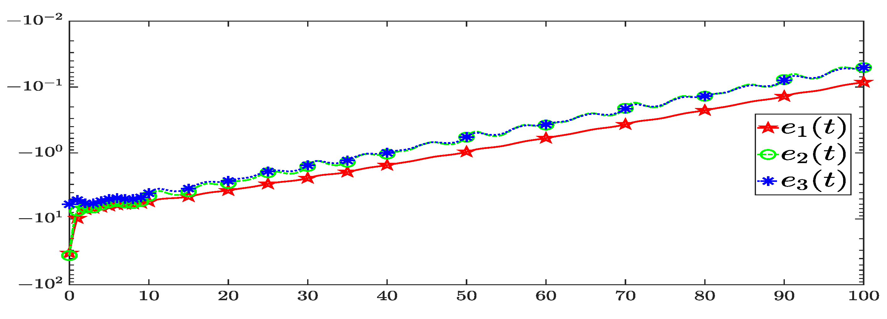
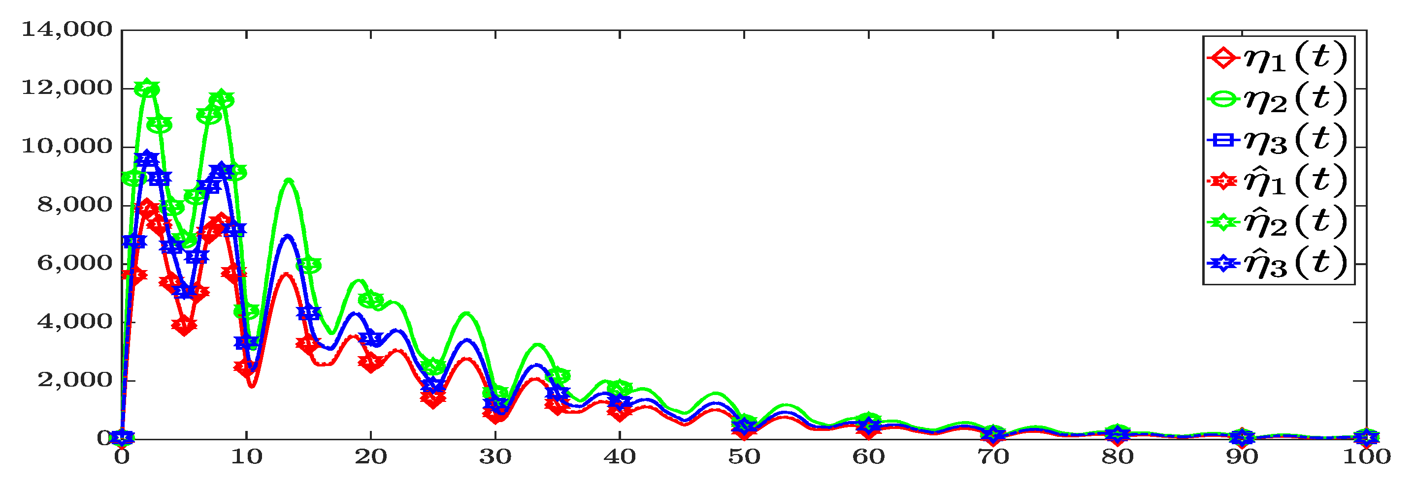
Give u ( t ) = 200 e 0.05 t | sin ( 0.2 π t ) | | cos ( 0.15 π t ) | . Under different initial conditions, the state trajectories of η ( t ) and the observed signal η ^ ( t ) are shown in Figure 2. The corresponding error signal e ( t ) = η ( t ) η ^ ( t ) is given in Figure 3. It can be observed from Figure 2 that all observer states ( η ^ 1 ( t ) , η ^ 2 ( t ) , η ^ 3 ( t ) ) remain in positive orthant when the conditions are satisfied in Theorem 1. Moreover, it can be obtained that the observer errors e ( t ) asymptotically converge to zero from Figure 3. Figure 2 and Figure 3 show that the state and disturbance observers design for system (1) with structural disturbance is effective.
In order to prove that the state observer obtained by Theorem 1 has a good performance, another input u ( t ) = 10,000 e 0.05 t | sin ( 0.2 π t ) | | cos ( 0.15 π t ) | is given and the simulation results obtained are shown in Figure 4. By comparing Figure 2 with Figure 4, it can be found that the simultaneous state and disturbance observers designed in Theorem 1 are all effective for different inputs.
Example 2.
Consider the system (1) with
A = 13.08 5.08 5.30 5.62 12.38 4.50 4.98 4.68 11.98 , B = 0.38 0.56 0.39 0.60 0.46 0.35 , C = 0.68 0.39 0.35 0.41 0.32 0.33 , E = 0.1950 0.1755 0.1800 0.1620 0.1400 0.1260 .
By Theorem 2, the gain matrices are:
G = 10.7958 0.0070 0.0115 10.2686 , Q = 0.0099 0.1400 0.0050 0.0213 , W = 6.2873 5.2919 1.4874 3.1204 , L = 1.3829 0.0125 0.9604 0.0256 .
Give u ( t ) = 100 e 0.05 t | sin ( 0.2 π t ) | | cos ( 0.15 π t ) | and w ( t ) = 75 e 0.05 t | cos ( 0.1 π t ) | | sin ( 0.15 π t ) | . Under differential initial conditions, the state trajectories of η ( t ) and the observed signal η ^ ( t ) are depicted in Figure 5. The corresponding error signal e ( t ) = η ( t ) η ^ ( t ) is shown in Figure 6. It can be seen from Figure 5 that all observer states ( η ^ 1 ( t ) , η ^ 2 ( t ) , η ^ 3 ( t ) ) remain in positive orthant when the conditions are satisfied in Theorem 2. Besides, it can be obtained that the observer errors e ( t ) asymptotically converge to zero from Figure 6. Figure 5 and Figure 6 show that the unknown input observer design for system (1) with non-structural disturbance is effective.
Different input and disturbance with u ( t ) = 10,000 e 0.05 t | sin ( 0.2 π t ) | | cos ( 0.15 π t ) | and w ( t ) = 7500 e 0.05 t | cos ( 0.1 π t ) | | sin ( 0.15 π t ) | are re-selected for simulation. The simulation results are shown in Figure 7. By comparing Figure 5 with Figure 7, it can be found that the unknown input observer designed in Theorem 2 is effective for different input and disturbance.

5. Conclusions

This paper proposes two classes of observers for positive systems with disturbance. One is for the structural disturbance and the other one is the non-structural disturbance. A novel designed approach without additional conditions on the observer gain matrices is introduced, which removes the limitation of gain performance and thus improves the accuracy of the observer. The observer frameworks proposed in this paper are universal to positive systems with structural/non-structural disturbance and the proposed design method can provide valuable reference for the control synthesis of positive systems. In addition, linear programming is used to solve the presented conditions, which greatly reduces the computational complexity. In future work, it will be interesting to develop symmetry observer [37] and sliding mode observer [38] to positive systems.

Author Contributions

Conceptualization, X.Z. and J.Z.; Methodology, L.H., X.Z., F.L. and J.Z.; Software, L.H. and F.L.; Validation, X.Z.; Formal analysis, X.Z.; Investigation, L.H. and J.Z.; Resources, X.Z.; Writing—original draft, L.H.; Writing—review & editing, F.L. and J.Z.; Visualization, F.L.; Funding acquisition, J.Z. All authors have read and agreed to the published version of the manuscript.

Funding

This work was supported by the National Nature Science Foundation of China (62073111), the Fundamental Research Funds for the Provincial Universities of Zhejiang (GK229909299001-010 and GK219909299001-002), and Graduate Scientific Research Foundation of Hangzhou Dianzi University (CXJJ2022153 and CXJJ2022163).

Institutional Review Board Statement

Not applicable.

Informed Consent Statement

Not applicable.

Data Availability Statement

Not applicable.

Conflicts of Interest

The authors declare no conflict of interest. The funders had no role in the design of the study; in the collection, analyses, or interpretation of data; in the writing of the manuscript, or in the decision to publish the results.

References

  1. Luenberger, D.G. Observing the state of a linear system. IEEE Trans. Mil. Electron. 1964, 8, 74–80. [Google Scholar] [CrossRef]
  2. Fortmann, T.; Williamson, D. Design of low-order observers for linear feedback control laws. IEEE Trans. Autom. Control 1972, 17, 301–308. [Google Scholar] [CrossRef]
  3. Lien, C.H. Robust observer-based control of systems with state perturbations via LMI approach. IEEE Trans. Autom. Control 2004, 49, 1365–1370. [Google Scholar] [CrossRef]
  4. Rajamani, R. Observers for Lipschitz nonlinear systems. IEEE Trans. Autom. Control 1998, 43, 397–401. [Google Scholar] [CrossRef]
  5. Efimov, D.; Raïssi, T.; Chebotarev, S.; Zolghadri, A. Interval state observer for nonlinear time varying systems. Automatica 2013, 49, 200–205. [Google Scholar] [CrossRef] [Green Version]
  6. Tranninger, M.; Seeber, R.; Zhuk, S.; Steinberger, M.; Horn, M. Detectability analysis and observer design for linear time varying systems. IEEE Control Syst. Lett. 2019, 4, 331–336. [Google Scholar] [CrossRef]
  7. Liu, Y.; Zhang, J. Reduced-order observer-based control design for nonlinear stochastic systems. Syst. Control Lett. 2004, 52, 123–135. [Google Scholar] [CrossRef]
  8. Eltag, E.; Aslam, M.S.; Chen, Z. Functional observer-based T-S fuzzy systems for quadratic stability of power system synchronous generator. Int. J. Fuzzy Syst. 2020, 22, 172–180. [Google Scholar] [CrossRef]
  9. Zhao, X.; Liu, H.; Zhang, J.; Li, H. Multiple-mode observer design for a class of switched linear systems. IEEE Trans. Autom. Sci. Eng. 2013, 12, 272–280. [Google Scholar] [CrossRef]
  10. Chen, M.S.; Chen, C.C. Robust nonlinear observer for Lipschitz nonlinear systems subject to disturbances. IEEE Trans. Autom. Control 2007, 52, 2365–2369. [Google Scholar] [CrossRef]
  11. Penarrocha, I.; Sanchis, R.; Albertos, P. H observer design for a class of nonlinear discrete systems. Eur. J. Control 2009, 15, 157–165. [Google Scholar] [CrossRef]
  12. Guan, Y.; Saif, M. A novel approach to the design of unknown input observers. IEEE Trans. Autom. Control 1991, 36, 632–635. [Google Scholar] [CrossRef]
  13. Zheng, G.; Bejaranoo, F.J.; Perruquetti, W.; Richard, J.P. Unknown input observer for linear time-delay systems. Automatica 2015, 61, 35–43. [Google Scholar] [CrossRef] [Green Version]
  14. Chen, W.H. Disturbance observer based control for nonlinear systems. IEEE/ASME Trans. Mechatron. 2004, 9, 706–710. [Google Scholar] [CrossRef] [Green Version]
  15. Yong, S.Z.; Zhu, M.; Frazzoli, E. Simultaneous input and state estimation for linear time-varying continuous-time stochastic systems. IEEE Trans. Autom. Control 2016, 62, 2531–2538. [Google Scholar] [CrossRef]
  16. Farina, L.; Rinaldi, S. Positive Linear Systems: Theory and Applications; John Wiley & Sons: Hoboken, NJ, USA, 2000. [Google Scholar]
  17. Kaczorek, T. Positive 1D and 2D Systems; Springer: London, UK, 2001. [Google Scholar]
  18. Fornasini, E.; Valcher, M.E. Stability and stabilizability criteria for discrete-time positive switched systems. IEEE Trans. Autom. Control 2011, 57, 1208–1221. [Google Scholar] [CrossRef]
  19. Briat, C. Robust stability and stabilization of uncertain linear positive systems via integral linear constraints: L1-gain and L-gain characterization. Int. J. Robust Nonlinear Control 2013, 23, 1932–1954. [Google Scholar] [CrossRef]
  20. Rami, M.A.; Tadeo, F.; Helmke, U. Positive observers for linear positive systems, and their implications. Int. J. Control 2011, 84, 716–725. [Google Scholar] [CrossRef]
  21. Ebihara, Y.; Peaucelle, D.; Arzelier, D. Analysis and synthesis of interconnected positive systems. IEEE Trans. Autom. Control 2016, 62, 652–667. [Google Scholar] [CrossRef] [Green Version]
  22. Zhang, J.; Zheng, G.; Feng, Y.; Chen, Y. Event-triggered state-feedback and dynamic output-feedback control of positive Markovian jump systems with intermittent faults. IEEE Trans. Autom. Control 2022. [Google Scholar] [CrossRef]
  23. Blanchini, F.; Colaneri, P.; Valcher, M.E. Co-positive Lyapunov functions for the stabilization of positive switched systems. IEEE Trans. Autom. Control 2012, 57, 3038–3050. [Google Scholar] [CrossRef]
  24. Knorn, F.; Mason, O.; Shorten, R. On linear co-positive Lyapunov functions for sets of linear positive systems. Automatica 2009, 45, 1943–1947. [Google Scholar] [CrossRef] [Green Version]
  25. Rami, M.A.; Tadeo, F. Controller synthesis for positive linear systems with bounded controls. IEEE Trans. Circuits Syst. II Express Briefs 2007, 54, 151–155. [Google Scholar] [CrossRef]
  26. Shao, S.Y.; Chen, M.; Wu, Q.X. Stabilization control of continuous-time fractional positive systems based on disturbance observer. IEEE Access 2016, 4, 3054–3064. [Google Scholar] [CrossRef]
  27. Li, P.; Lam, J. Positive state-bounding observer for positive interval continuous-time systems with time delay. Int. J. Robust Nonlinear Control 2012, 22, 1244–1257. [Google Scholar] [CrossRef]
  28. Zaidi, I.; Chaabane, M.; Tadeo, F.; Benzaouia, A. Static state-feedback controller and observer design for interval positive systems with time delay. IEEE Trans. Circuits Syst. II Express Briefs 2014, 62, 506–510. [Google Scholar] [CrossRef]
  29. Zhang, J.; Zhang, R.; Chen, Y.; Fu, S. Linear programming based dynamic output-feedback controller for positive systems. In Proceedings of the 2017 American Control Conference (ACC), Seattle, WA, USA, 24–26 May 2017; pp. 1281–1290. [Google Scholar]
  30. Qi, W.; Park, J.H.; Zong, G.; Cao, J.; Cheng, J. A fuzzy Lyapunov function approach to positive L1 observer design for positive fuzzy semi-Markovian switching systems with its application. IEEE Trans. Syst. Man Cybern. Syst. 2018, 51, 775–785. [Google Scholar] [CrossRef]
  31. Zhang, D.; Zhang, Q.; Du, B. L1 fuzzy observer design for nonlinear positive Markovian jump system. Nonlinear Anal. Hybrid Syst. 2018, 27, 271–288. [Google Scholar] [CrossRef]
  32. Arogbonlo, A.; Huynh, V.T.; Oo, A.M.T.; Trinh, H. Functional observers design for positive systems with delays and unknown inputs. IET Control Theory Appl. 2020, 14, 1656–1661. [Google Scholar] [CrossRef]
  33. Oghbaee, A.; Shafai, B.; Nazari, S. Complete characterisation of disturbance estimation and fault detection for positive. IET Control Theory Appl. 2018, 12, 883–891. [Google Scholar] [CrossRef]
  34. Ocampo-Martínez, C.; Puig, V.; Cembrano, G.; Creus, R.; Minoves, M. Improving water management efficiency by using optimization-based control strategies: The Barcelona case study. Water Sci. Technol. Water Supply 2009, 9, 565–575. [Google Scholar] [CrossRef]
  35. Ocampo-Martínez, C.; Puig, V.; Cembrano, G.; Quevedo, J. Application of predictive control strategies to the management of complex networks in the urban water cycle. IEEE Control Syst. Mag. 2013, 3, 15–41. [Google Scholar]
  36. Zhang, J.; Yang, H.; Li, M.; Wang, Q. Robust model predictive control for uncertain positive time-delay systems. Int. J. Control. Autom. Syst. 2019, 17, 307–318. [Google Scholar] [CrossRef]
  37. Bonnabel, S.; Martin, P.; Rouchon, P. Symmetry-preserving observers. IEEE Trans. Auto-Matic Control 2008, 53, 2514–2526. [Google Scholar] [CrossRef] [Green Version]
  38. Edwards, C.; Spurgeon, S.K.; Patton, R.J. Sliding mode observers for fault detection and isolation. Autom. Autom. 2000, 36, 541–553. [Google Scholar] [CrossRef]
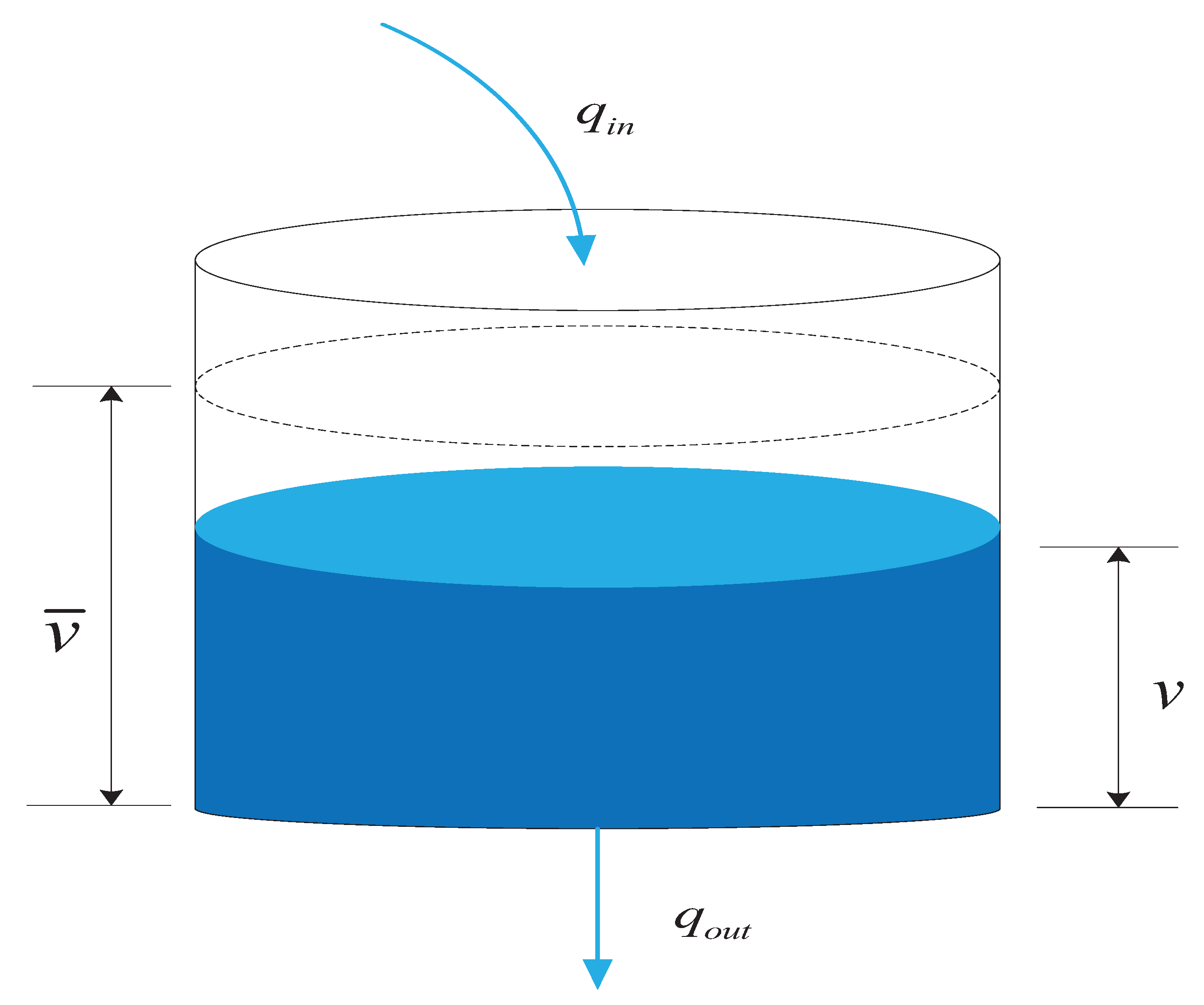
Figure 1. The virtual tank.
Mathematics 11 00200 g001
Figure 2. The state trajectories of system (1).
Mathematics 11 00200 g002
Figure 3. The corresponding error trajectories of system (1).
Mathematics 11 00200 g003
Figure 4. The state trajectories of system (1) with input u ( t ) .
Mathematics 11 00200 g004
Figure 5. The state trajectories of system (1).
Mathematics 11 00200 g005
Figure 6. The corresponding error trajectories of system (1).
Mathematics 11 00200 g006
Figure 7. The state trajectories of system (1) with input u ( t ) and disturbance w ( t ) .
Mathematics 11 00200 g007
Disclaimer/Publisher’s Note: The statements, opinions and data contained in all publications are solely those of the individual author(s) and contributor(s) and not of MDPI and/or the editor(s). MDPI and/or the editor(s) disclaim responsibility for any injury to people or property resulting from any ideas, methods, instructions or products referred to in the content.