Article

Cost-Sensitive Laplacian Logistic Regression for Ship Detention Prediction

1
Department of Logistics & Maritime Studies, The Hong Kong Polytechnic University, Hung Hom, Hong Kong 999077, China
2
Faculty of Business, The Hong Kong Polytechnic University, Hung Hom, Hong Kong 999077, China
*
Author to whom correspondence should be addressed.
Mathematics 2023, 11(1), 119; https://doi.org/10.3390/math11010119
Submission received: 21 November 2022 / Revised: 19 December 2022 / Accepted: 23 December 2022 / Published: 27 December 2022

Abstract

:
Port state control (PSC) is the last line of defense for substandard ships. During a PSC inspection, ship detention is the most severe result if the inspected ship is identified with critical deficiencies. Regarding the development of ship detention prediction models, this paper identifies two challenges: learning from imbalanced data and learning from unlabeled data. The first challenge, imbalanced data, arises from the fact that a minority of inspected ships were detained. The second challenge, unlabeled data, arises from the fact that in practice not all foreign visiting ships receive a formal PSC inspection, leading to a missing data problem. To address these two challenges, this paper adopts two machine learning paradigms: cost-sensitive learning and semi-supervised learning. Accordingly, we expand the traditional logistic regression (LR) model by introducing a cost parameter to consider the different misclassification costs of unbalanced classes and incorporating a graph regularization term to consider unlabeled data. Finally, we conduct extensive computational experiments to verify the superiority of the developed cost-sensitive semi-supervised learning framework in this paper. Computational results show that introducing a cost parameter into LR can improve the classification rate for substandard ships by almost 10%. In addition, the results show that considering unlabeled data in classification models can increase the classification rate for minority and majority classes by 1.33% and 5.93%, respectively.

1. Introduction

Maritime transportation is the backbone of international trade [1]. To guarantee maritime safety, as a complement to numerous international regulations and conventions, the port state control (PSC) is seen as the last line of defense against substandard ships [2]. During a PSC inspection, a ship condition found not to be compliant with the relevant regulations and conventions is recorded as a deficiency item. If critical deficiency items are found by port state control officers (PSCOs), the port state can detain the high-risk ship and require the ship to rectify these deficiency items before its departure. For ship operators, ship detention is the most severe outcome of a PSC inspection because it delays shipping schedules [3], and maritime transportation delays are costly [4]. For port states, identifying as many ships as possible that should be detained is their principal task because failing to identify these high-risk ships may lead to marine accidents with serious social and environmental damages. Hence, identifying ships with a high probability of being detained is of great practical significance. However, inaccuracies and inefficiencies are always present at several stages during a PSC inspection, from selecting a ship to making a final decision [3]. For example, the current ship selection scheme is not efficient in targeting high-risk ships, and to what extent the ships should be inspected and the decision regarding detention are highly dependent on the subjectivity of PSCOs. Therefore, designing an intelligent decision support system to help predict ship detention risk is an urgent need.
Nowadays, many studies use machine learning (ML) methods and PSC data to design inspection schemes for port authorities, examining how to implement PSC inspections more efficiently and discussing the effects of PSC inspections [5]. However, to the best of our knowledge, studies relevant to ship detention prediction are somehow limited. Different from most existing studies that focus on predicting the number of deficiencies of a ship, predicting ship detention is a more challenging task. As reported in the Annual Report on Port State Control in the Asia-Pacific Region 2021, out of 22,730 inspections which involve 14,951 individual ships operating in the region, 11,567 inspections found ships with deficiencies, while only 526 ships were eventually detained  [6]. From this report, we identify two challenges when developing classification models for ship detention prediction. First, in the region, the deficiency rate was 51%, while the detention rate was only 2.31%, showing that the ship detention rate is much more imbalanced than the ship deficiency rate. This result requires us to learn from imbalanced data, where the distribution of examples is skewed since representatives of undetained ships appear much more frequently [7]. In addition, less than 60% of all ships are inspected, so we must learn from unlabeled data; that is, not all visiting ships are labeled with inspection results. To address each of the two challenges, this paper studies two machine learning paradigms for ship detention prediction: cost-sensitive learning and semi-supervised learning.
Class imbalance and cost-sensitive learning are closely related to each other [8,9]. Cost-sensitive learning aims to make the optimal decision that minimizes the misclassification cost [10,11,12,13]. For our studied problem, misclassifying a ship that should be detained and misclassifying a ship that should not be detained have different influences. Therefore, the two kinds of misclassifications should be considered with different costs. Several studies have shown that cost-sensitive methods performed better than sampling methods in certain application domains [14,15,16,17]. Semi-supervised learning aims to improve learning performance by exploiting the unlabeled data in addition to the labeled data [18,19]. The lack of an assigned inspection class for each foreign visiting ship is the issue we are faced with when using observational data in PSC-related studies. This naturally occurs because ships that appear at high risk of detention have high possibilities of being inspected, while ships at lower risk may not. For example, the Paris Memorandum of Understanding (MoU) and Tokyo MoU adopt ship risk profile (SRP) to select ships that are more likely to have larger numbers of deficiencies and detained possibilities. Therefore, the PSC dataset used for prediction is a biased collection of all foreign visiting ships, which may ignore some important and valuable information underlying the unlabeled data.
The use of unlabeled data in cost-sensitive learning has attracted growing attention and many frameworks have been developed [20,21,22,23]. To the best of our knowledge, there has not been an attempt to apply both semi-supervised learning and cost-sensitive learning to help improve ship detention prediction. In our paper, we aim to address unequal misclassification costs and utilize unlabeled data simultaneously based on an extension of logistic regression (LR) by introducing a cost parameter and using data-dependent graph regularization [24]. Through computational experiments, the superiority of the proposed cost-sensitive semi-supervised learning framework in ship detention prediction is verified.
The remainder of this paper is organized as follows. Section 2 reviews related studies on ship detention prediction. Section 3 introduces the preliminaries of the ML framework to be extended, including the basic concepts of a learning problem and the Laplacian operator of a graph. Section 4 develops the cost-sensitive semi-supervised learning framework for ship detention prediction and introduces the performance metrics of prediction models. Section 5 conducts computational experiments to show the benefits of our developed cost-sensitive semi-supervised learning framework. Finally, Section 6 concludes this study and proposes future research directions.

2. Literature Review

Because current SRP schemes do not efficiently identify substandard ships, most PSC-related studies have focused on improving inspection efficiency by developing methods for identifying ships with more deficiencies or higher detention probabilities. Recall that the detention rate is much more imbalanced than the deficiency rate, and predicting the total number of deficiencies of a ship or predicting the number of deficiencies under each category is much easier than predicting the detention probability. The summary of the literature on ship risk prediction is shown in Table 1. We first briefly review studies focusing on predicting ship deficiency number. Early studies, such as Xu et al. [25] and Xu et al. [26], used a support vector machine (SVM) to predict the overall ship risk considering the ship deficiency number. Gao et al. [27] combined k-nearest neighbor (kNN) and SVM. In recent years, there are an increasing number of studies developing more advanced ML methods for ship deficiency number prediction. Wang et al. [28] developed a tree-augmented naive (TAN) Bayes classifier to predict the number of deficiencies of each foreign visiting ship. Chung et al. (2020) [29] and Yan et al. [30] adopted the Apriori algorithm to determine the type and sequence of deficiency codes that should be inspected. In recent years, ship deficiency prediction models have also been used to solve inspection assignment problems, as studied by Yan et al. [31] and Yan et al. [32]. For more studies related to ship deficiency number prediction, readers can refer to Yan et al. [33].
We now proceed to review related studies on ship detention prediction. According to Wu et al. [34], there is a stream of studies focusing on analyzing the relationship between the identified ship deficiencies and the detention outcome, such as Cariou and Wolff [35], Chen et al. [36], and Yan and Wang [37]. However, these studies did not consider the influence of ship parameters (e.g., ship age and ship type) on ship detention outcome. Ship parameters serve as critical factors in ship detention. Cariou et al. [38] pointed out that ship age is the main contributor to the ship detention. The same observation has also been shown by Tsou [39] and Şanlıer [40]. Hänninen and Kujala [41] identified that the ship type, the deficiency number, and the PSC inspection type are the most important factors attributed to the ship detention. Yang et al. [42] proposed a data-driven Bayesian network (BN) model based on TAN learning to predict the ship detention probability of bulk carriers under the Paris MoU. To determine the optimal inspection policy for a port, Yang et al. [43] incorporated the results of the ship detention prediction model into a game model that considered both port authorities and ship operators. Wu et al. [34] used an SVM model to predict ship detention, where they selected input features by using an analytic hierarchy process (AHP) and a grey relational analysis (GRA) to improve prediction accuracy. However, the ship detention prediction models seldom considered the imbalanced ship detention rate. To remedy this issue, Yan et al. [3] used a balanced random forest (BRF) model to predict ship detention to address the issues caused by the low-probability detention outcome, which is based on the sampling technique.
In summary, although some studies have detention prediction models, the two identified challenges mentioned before are seldom considered by them. First, they did not consider that the dataset for ship detention prediction is highly imbalanced, so we should attach different misclassification costs for minority and majority classes. Second, they did not consider that the used dataset is a biased collection of all foreign visiting ships, so we should further consider the value of unlabeled data. Therefore, to bridge these two research gaps, this paper develops the cost-sensitive semi-supervised learning framework for targeted and cost-effective ship detention prediction.

3. Preliminaries

This section introduces preliminaries that are related to this research. We first illustrate the importance of the regulation term in a learning problem in Section 3.1. We then introduce the smoothness of a decision function and the Laplacian operator of a graph in Section 3.2. The introduction generally follows the approaches from Vapnik [44], Shalev-Shwartz and Ben-David [45], and Melas-Kyriazi [46].

3.1. The Learning Problem and Regularization

Before proceeding to the introduction of a semi-supervised learning problem, this section first focuses on a supervised setting to lay some foundations of ML algorithms that would be extended in subsequent sections. Consider we have a dataset S = { ( x 1 , y 1 ) , …, ( x i , y i ) , , ( x n , y n ) } , where x i X R d is the feature vector and y i Y R is the corresponding label. We assume that our data ( x i , y i ) are independently drawn and identically distributed from a probability space X × Y with measure ρ . Learning is to find a function f that generalizes from this finite dataset S to the space X × Y . This task can be achieved by minimizing the expected loss ϵ , also called the risk:
ϵ ( f , x , y ) = E [ L ( y , f ( x ) ) ] = X × Y L ( y , f ( x ) ) d ρ ( x , y ) ,
where L ( y , f ( x ) ) denotes the loss function that measures how well the function f ( x ) predicts the outcome. If f ( x ) = y , L ( y , f ( x ) ) = 0 and this prediction is perfect. Then, the objective of learning is to find a function by minimizing the risk:
f * = arg min f F X × Y L ( y , f ( x ) ) d ρ ( x , y ) ,
where F denotes the class of all measurable functions. Because we only have finite data and computing (2) is impossible, we approximate it by using the empirical risk:
ϵ ^ ( f , x , y ) = 1 n i = 1 n L ( y i , f ( x i ) ) X × Y L ( y , f ( x ) ) d ρ ( x , y ) .
If we could minimize the empirical risk over all functional functions f F , we would be able to approximate X × Y L ( y , f ( x ) ) d ρ ( x , y ) and obtain a function f ^ = arg min f F ϵ ^ ( f , x , y ) resembling the perfect function f * . However, this is not possible because we are learning in an entirely unconstrained setting where the distributions of the dataset and the class of functions are not assumed in advance. To overcome this issue, we can take either of two ways accordingly to constrain the learning problem: (1) by assuming that the dataset follows a class of probability distributions θ , namely letting ρ θ , or (2) by assuming that learning functions follow a limited class of target functions H , namely letting f H , where H is a subset of F . Because the probability distribution of ρ is hardly known in practice, this paper adopts the second approach, as is common in ML theory.
When we optimize over a restricted class of functions H , we would like H to be large so that we can learn complex functions. However, these complex functions may not work well with new data if they fit our training data nearly perfectly, causing a problem known as overfitting. Generally, when we have a lot of data, we hope to learn complex functions. Conversely, when we have little data, we prefer simpler functions. In order to achieve this aim, the regularization term is always introduced into the loss function, which takes the form of a penalty R and biases learning toward simpler and smoother functions. With regularization, the learning problem is transformed into:
min f H ϵ ^ ( f , x , y ) + λ R ( f , x , y ) ,
where H is the predefined space, and λ > 0 is a hyperparameter that balances the empirical risk term and the regularization term. Generally, the regularization term only depends on the function f and its parameters (e.g., L1/L2 norms). We call this regularization term a data-independent regularization term. In addition, in order to enforce that a prediction model should output similar prediction results for a pair of similar examples no matter whether they are labeled or unlabeled, we introduce a graph regularization term into the semi-supervised learning problem that this paper studies. Graph regularization is an example of data-dependent regularization because it is formulated by examining the geometric features of labeled and unlabeled data. We will introduce it in Section 3.2 and Section 4.3.

3.2. Smoothness and Laplacian

Our research problem focuses on the semi-supervised learning setting, where we wish to learn the probability distribution based on which both labeled and unlabeled examples are drawn. Assuming that the underlying distribution may have non-trivial geometric features, we hope to design algorithms that can exploit these geometric features to facilitate the learning outcome [24]. Because we have discrete and finite data, we assume that the probability distribution may have support on a graph, where we regard data examples as nodes. To examine the geometric features of a graph, we need to introduce the definition of the smoothness of a decision function on a graph and the Laplacian operator of a graph.
Consider G = ( N , E ) as a connected and undirected graph with edges E = { 1 , , E } and nodes N = { 1 , , N } . We denote by W = ( w i j ) i , j = 1 N the symmetric weighted adjacency matrix on graph G , where w i j measures the similarity between nodes i and j [47], and D = diag ( d 1 , , d N ) the degree matrix with degrees d i = j = 1 N w i j , i = 1 , , N on the diagonal. A real-valued function on G is a map f : N R defined on the nodes of the graph. Intuitively, a function on a weighted graph is smooth if its value on a node is similar to its value on each of the node’s neighbors; that is, this function does not make too many “jumps’’ [46]. Following this notion, we use
i = 1 N j = 1 N w i j f i f j 2
to measure the smoothness of a function on a weighted graph, which measures the weighted differences between the function value of a node with those of its neighbors. Because (5) is symmetric and quadratic, we can rewrite it as:
i = 1 N j = 1 N w i j f i f j 2 = i = 1 N j = 1 N w i j f i 2 2 f i f j w i j + w i j f j 2 = i = 1 N d i f i 2 2 i = 1 N j = 1 N f i f j w i j + j = 1 N d j f j 2 = 2 i = 1 N d i f i 2 2 i = 1 N j = 1 N f i f j w i j = 2 f D f 2 f W f = 2 f ( D W ) f = 2 f L f ,
where f = ( f 1 , f 2 , , f N ) , and L = D W . We call L the Laplacian of the graph G  [24,48].

4. Models and Algorithms

Based on the preliminaries mentioned above, this section introduces the cost-sensitive semi-supervised learning framework for ship detention prediction considering missing labels and class imbalance, namely the cost-sensitive Laplacian logistic regression (CosLapLR) framework. We first introduce the basic logistic regression model for supervised classification in Section 4.1 and expand this model by incorporating a graph regularization term and cost-sensitive techniques to develop a cost-sensitive semi-supervised learning framework in Section 4.2. Finally, we introduce performance metrics of classification models in Section 4.3.

4.1. Predictive Model

Recall that in Section 3.1 we have a dataset S = { ( x 1 , y 1 ) , , ( x i , y i ) , , ( x n , y n ) } . Here, in this study, we denote by x i X R d the feature vector of an inspected ship i and y i Y = { ± 1 } the corresponding binary detention outcome of ship i. For every feature vector x i , i = 1 , , n , the detention outcome is either y i = 1 or y i = 1 , where 1 corresponds to a detention result and 1 otherwise. We use logistic regression models to predict detention probabilities. The discriminative model for logistic regression is as follows:
P ( y i = ± 1 | x i , β ) = 1 1 + exp ( y i β x i ) ,
where β R d is the parameter vector that we should estimate by maximum likelihood estimation (MLE) by minimizing the conditional negative log-likelihood as follows:
log L ( β ) = log i = 1 n P ( y i = ± 1 | x i , β ) = i = 1 n log 1 + exp ( y i β x i ) .
By scaling (8) of factor 1 / n and assuming that f ( x i ) = β x i , we can obtain the empirical risk minimization problem with logistic loss, given as L y i , f ( x i ) = log 1 + exp y i β x i , as follows:
min β R d 1 n i = 1 n log 1 + exp y i β x i .
Finally, to avoid training a complex and overfitting decision function, we add a data-independent regularization term, λ H β β , into (9) as follows:
min β R d 1 n i = 1 n log 1 + exp y i β x i + λ H β β ,
where λ H > 0 is a hyperparameter balancing the empirical risk term and the regularization term.

4.2. Cost-Sensitive Semi-Supervised Learning Framework

To consider missing data for ships that did not receive PSC inspections, we add a graph regularization in (10) to impose an intrinsic constraint requiring that the decision function f ( x ) should be smooth in predicting the detention outcomes for ships with similar features. In addition to our existing dataset { ( x i , y i ) } i = 1 n , we assume that there is another dataset { x j } j = n + 1 n + u capturing the feature vectors of u uninspected ships. Because we do not know the marginal distribution from which uninspected ships are drawn, the empirical estimates of the geometric features in uninspected ships are represented as a graph. In this graph, there is a total of n + u nodes corresponding to all ships. These nodes represent the inspected (labeled) and uninspected (unlabeled) ships, and edge weights between nodes represent pairwise relationships between ships. If ship i is among the k-nearest neighbors of ship j, or vice versa, where k is a hyperparameter, these two ships are connected by a weighted edge, whose assigned weight is denoted by w i j (the approach to determining the value of w i j for two neighbors i and j will be introduced in Section 5); for two ships i and j that are not among the neighbors of each other, we set w i j = 0 . Therefore, by measuring the similarity of all ships (including inspected and uninspected ships), we can obtain a symmetric weighted adjacency matrix W = ( w i j ) i , j = 1 n + u and the Laplacian matrix L of this graph, denoted as L = W D , where D = diag j = 1 n + u w 1 j , , j = 1 n + u w ( n + u ) j represents the degree matrix. Then, adding the graph regularization term into (10), we can obtain
min β R d 1 n i = 1 n log 1 + exp y i β x i + λ H β β + λ G β X n + u L X n + u β ,
where X n + u = ( x 1 , , x n , x n + 1 , , x n + u ) is an ( n + u ) × d -dimensional matrix, and λ H and λ G represent the parameters that control the H norm and the intrinsic norm, respectively. Regarding (11), the log term measures the prediction error, the H norm term requires that the decision function should not be complex, and the Laplacian term (intrinsic norm) requires that the decision function should output similar detention outcomes for two ships with high similarity regardless of their inspection status.
From above analysis, we have illustrated how to consider uninspected ships in our prediction model. We now proceed to introduce how to address the issue of class imbalance in the ship detention prediction problem. Class imbalance is caused by the fact that among inspected ships, only a small proportion of ships are detained due to their identified serious deficiencies. The original formulation of (11) does not consider the class imbalance because it attaches the same costs of misclassifying a ship that should be detained and misclassifying a ship that should not be detained. However, in reality, the above two cases should be considered differently, i.e., attached with distinguished misclassification costs, because they have different outcomes and impacts. Specifically, if a ship with serious deficiencies is not detained and is regarded to be seaworthy, this ship is more likely to cause serious accidents while sailing, leading to possible economical and environmental damages. Conversely, if a ship without serious deficiencies is detained, it will cause a shipping delay to this ship. Generally, from a socially beneficial perspective, the overall possible cost of the former case is much larger than that of the latter case. To consider two different cases in the loss function, we introduce two partial losses, denoted as L 1 f ( x ) = log 1 + exp ( β x ) and L 1 f ( x ) = log 1 + exp ( β x ) , to construct a cost-sensitive classification loss given by L ϕ : { 1 , 1 } × R [ 0 , ] with cost parameter ϕ ( 0 , 1 ) as:
L ϕ = ϕ 1 { y = 1 } log 1 + exp β x + ( 1 ϕ ) 1 { y = 1 } log 1 + exp β x ,
where 1 { · } is an indicator function that equals 1 if the condition in the brackets is true and 0 otherwise. Accordingly, the cost-sensitive formulation of optimization problem (11) is as follows:
min β R d 1 n i = 1 n ϕ 1 { y i = 1 } log 1 + exp β x i + ( 1 ϕ ) 1 { y i = 1 } log 1 + exp β x i + λ H β β + λ G β X n + u L X n + u β .
In order to linearize the indicator function, the equivalent optimization problem of (12) is finally as follows:
min β R d 1 2 n ϕ ( 1 + y ) log 1 + exp X n β + ( 1 ϕ ) ( 1 y ) log 1 + exp X n β + λ H β β + λ G β X n + u L X n + u β ,
where X n = ( x 1 , , x n ) is an n × d -dimensional matrix, 1 is an n × 1 -dimensional vector with elements 1, and y = ( y 1 , , y n ) is an n × 1 -dimensional vector with labels y i , i { 1 , , n } . In summary, the developed CosLapLR framework is given in Algorithm 1.
Algorithm 1: Cost-sensitive Laplacian Logistic Regression (CosLapLR).
Require:n inspected ships { ( x i , y i ) } i = 1 n , u uninspected ships { x j } j = n + 1 n + u .
Ensure: Estimated decision function f : R d R .
1:
Step 1: Choose the hyperparameter k and construct the symmetric weighted adjacency matrix W with n + u nodes and compute edge weights w i j by k-nearest neighbors.
2:
Step 2: Compute the Laplacian matrix L = D W , where D = diag ( j = 1 n + u w 1 j , , j = 1 n + u w ( n + u ) j ) .
3:
Step 3: Choose the regularization parameters λ H , λ G , and the cost parameter ϕ .
4:
Step 4: Solve (14) to obtain β * .
5:
Step 5: Output function f * ( x ) = β * x .

4.3. Performance Metrics

Common evaluation metrics for binary classification problems are true negative (TN), false positive (FP), false negative (FN), and true positive (TP) [3]. For classifiers used for balanced datasets, model accuracy, denoted as a c c , is the most commonly used metric to evaluate the model performance, which is defined as follows:
a c c = T P + T N T P + F P + F N + T N .
However, this metric is not suitable to evaluate the prediction performance of classifiers developed for imbalanced and cost-sensitive learning. Because our aim is to obtain a higher identification rate for substandard ships that should be detained without greatly compromising the classification of ships that are not substandard, we mainly use sensitivity and specificity to evaluate the classification performance of classifiers [49]. Sensitivity, or true positive rate ( T P F N + T P ), denoted as s e n , represents the accuracy on the positive class; specificity ( T N F P + T N ), or true negative rate, denoted as s p e , represents the accuracy on negative class. Furthermore, based on the cost-sensitive perspective, we design a cost-sensitive evaluation metric, called decision loss (DL) metric, to evaluate the overall misclassification costs of a prediction model, which is related to the cost parameter ϕ and the values of false negative (FN) and false positive (FP), shown as follows:
D L = ϕ × F N + ( 1 ϕ ) × F P .

5. Computational Experiments

This section conducts extensive computational experiments to verify the superiority of the proposed cost-sensitive semi-supervised learning framework. We first introduce the dataset we use and the parameter settings in Section 5.1. We then draw trade-off curves to determine Pareto-optimal prediction models in Section 5.2.1 and then determine cost-effective models based on the minimum value of DL in Section 5.2.2.

5.1. Data Description

The dataset we use in this study consists of two parts, namely the labeled one and the unlabeled one. The labeled one contains 3026 records of PSC initial inspections during January 2015 to December 2019 period at the Hong Kong Port and the corresponding ship-related factors. Note that among 3026 inspections, only 100 inspections were labeled with detention outcomes. The PSC inspection records are retrieved from the Asia Pacific Computerized Information System (APCIS) (http://apcis.tmou.org/public/, accessed on 15 October 2022) provided by Tokyo MoU, and the ship-related factors are obtained from the World Shipping Register (WSR) (http://world-ships.com/, accessed on 15 October 2022) database. The unlabeled one contains 2675 records of incoming foreign ships during January 2021 to December 2021 at the Hong Kong port (the corresponding database only provides records starting from 12 September 2020) and the corresponding historical inspection information and ship-related factors. The records of incoming foreign ships are downloaded from the website of the Hong Kong government (https://data.gov.hk/en-data/dataset/hk-md-mardep-vessel-arrivals-and-departures, accessed on 15 October 2022), the corresponding historical inspection information is retrieved from the APCIS database, and the ship-related factors are obtained from the WSR database as well.
We consider 14 input features that are strongly related to the ship condition in the literature [3,5,28,30,32], including ship age, gross tonnage, length, depth, beam, type, ship flag performance, ship recognized organization performance, and ship company performance in Tokyo MoU, last PSC inspection time in Tokyo MoU, the number of ship deficiencies in the last inspection in Tokyo MoU, the number of detentions in all historical PSC inspections, the number of flag changes, and whether a ship has a casualty in last 5 years [3,5,28,30,32]. We follow the data preprocessing procedures of Yan et al. [31]. All continuous attributes were normalized to a mean of zero and a standard deviation of one. We use the scipy.optimize package (https://docs.scipy.org/doc/scipy/reference/optimize.html, accessed on 15 October 2022) in Python as the optimization solver.
We define the weight matrix W by k-nearest neighbors for CosLapLR models as follows [24,47]:
w i j = e γ x i x j , if x i , x j are neighbors 0 , otherwise .
We assume that in practice the cost parameter ϕ is predefined by the stakeholders (i.e., port authorities) who generally weigh the misclassification of substandard ships much higher than low-risk ships. We will conduct experiments for varying choices of cost parameter ϕ to show its effect in Section 5.2.1. Therefore, under each cost parameter ϕ , there are four other hyperparameters in total in CosLapLR models, namely, γ , k, λ H , and λ G . Before training ML models, we randomly divide the labeled dataset into a training set (70%, 2118 records) and a test set (30%, 908 records). We adopt 3-fold cross-validation (CV) in the model training process. Following the literature [49,50], the nearest neighbor parameter k is chosen from set {3,5,7}, the weight parameter γ from set { 2 i | 11 , 9 , 7 , 5 , 3 , 1 , 1 , 3 , 5 } , and the regularization parameters λ H and λ G from set { 2 i | 11 , 9 , 7 , 5 , 3 , 1 , 1 , 3 , 5 } and set { 2 i | 17 , 15 , 13 , 11 , 9 , 7 , 5 , 3 } , respectively.

5.2. Results

5.2.1. Pareto Frontier Graphs of Binary Classification Models

Recall that the aim of this study is to obtain a higher identification rate for substandard ships that should be detained without greatly compromising the classification of ships that are not substandard. Therefore, we draw trade-off curves to determine Pareto-optimal models based on sensitivity and specificity. Under Pareto optimality, a model is considered dominated if there is another model that has a higher sensitivity or a higher specificity [49]. For CosLapLR models, we draw Pareto frontier graphs consisting of non-dominated models for varying choices of the cost parameter ϕ based on the 3-fold CV performance. We conduct experiments for ϕ { 0.5 , 0.7 , 0.9 , 0.95 , 0.97 , 0.99 } , whose Pareto frontier graphs are shown in Figure 1, respectively. Figure 1 shows that increasing ϕ can improve sensitivity, namely the classification performance of substandard ships, without significantly sacrificing specificity, namely the classification performance of ships that are not substandard.
Furthermore, we also draw Pareto-frontier graphs of the following learning methods: LR, cost-sensitive logistic regression (CosLR), and Laplacian logistic regression (LapLR), whose learning problems are shown as follows:
[LR]
min β R d 1 2 n ( 1 + y ) log 1 + exp X n β + ( 1 y ) log 1 + exp X n β + λ H β β ,
[CosLR]
min β R d 1 2 n ϕ ( 1 + y ) log 1 + exp X n β + ( 1 ϕ ) ( 1 y ) log 1 + exp X n β + λ H β β ,
[LapLR]
min β R d 1 2 n ( 1 + y ) log 1 + exp X n β + ( 1 y ) log 1 + exp X n β + λ H β β + λ G β X n + u L X n + u β .
For these learning models, corresponding hyperparameters, such as γ , k, λ H , λ G , and ϕ , follow the same search sets stated above.
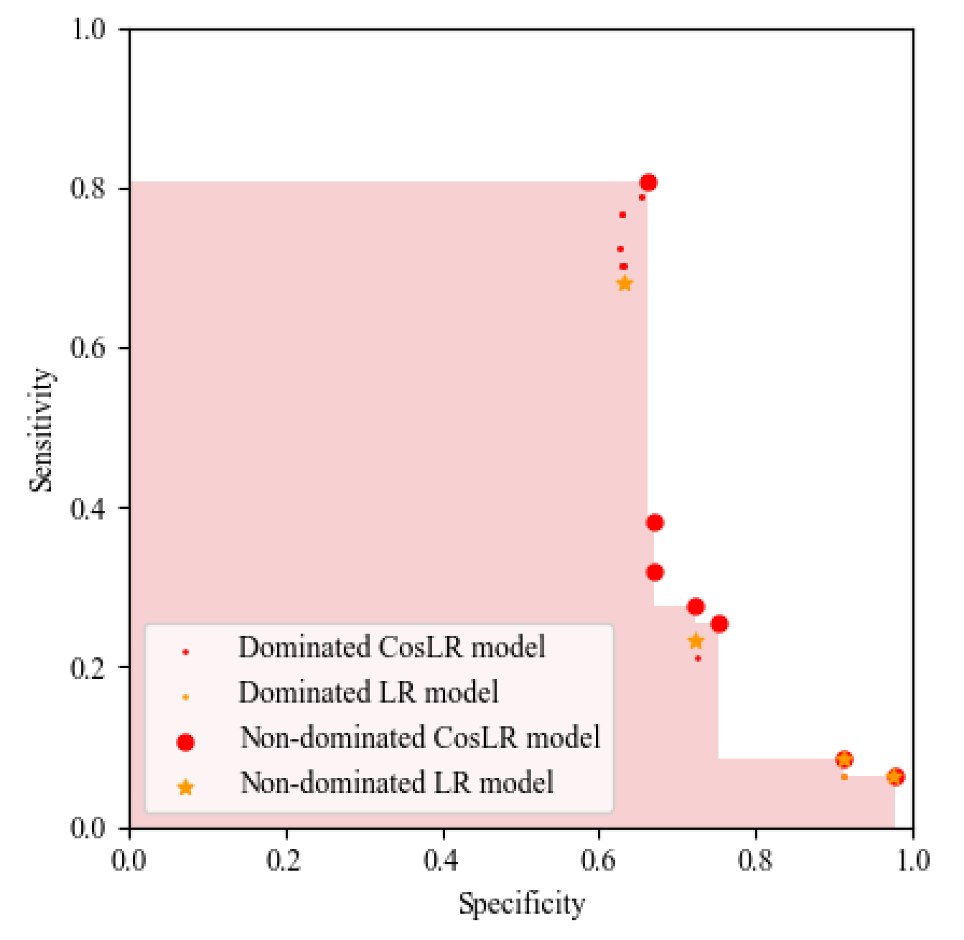
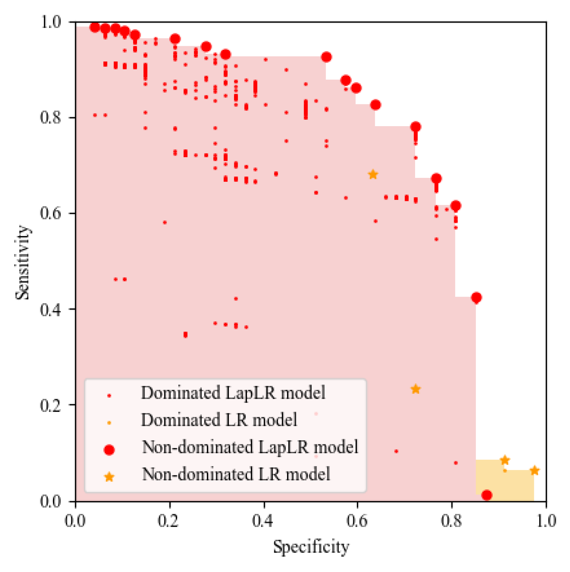
After observing the Pareto frontier graph of LR models and CosLR models, as shown in Figure 2, we can find that introducing a cost parameter into LR can improve the value of sensitivity by almost 0.1, leading to a higher classification rate of substandard ships. Furthermore, after observing the Pareto frontier graph of LR models and LapLR models, as shown in Figure 3, we can find that considering unlabeled data into LR can improve the value of sensitivity without greatly compromising the value of specificity. Therefore, the significance of our proposed method is verified.

5.2.2. Prediction Performance of Binary Classification Models

From the above analysis, we have shown from Pareto frontier graphs that considering unlabeled data can expand the coverage of the Pareto frontier, and introducing the cost parameter can improve the classification ability for substandard ships without greatly compromising the classification ability for low-risk ships. We further pick up the models with the lowest DL value in each binary classification framework (i.e., LR, LapLR, CosLR, and CosLapLR) and list their hyperparameters and prediction performance metrics in Table 2.
As shown in Table 2, from a broad sense, the average increasing ratios of specificity and sensitivity of six groups of experiments are 1.33% ( ( 0.672 0.631 ) + ( 0.672 0.631 ) + ( 0.648 0.630 ) + ( 0.661 0.663 ) + ( 0.660 0.655 ) + ( 0.630 0.653 ) 6 × 100 % = 1.33 % ) and 5.93% ( ( 0.786 0.679 ) + ( 0.786 0.679 ) + ( 0.786 0.714 ) + ( 0.821 0.821 ) + ( 0.821 0.786 ) + ( 0.821 0.786 ) 6 × 100 % = 5.93 % ), respectively. This result verifies that considering unlabeled data in classification models can increase the classification ability for both minority and majority classes. Consequently, the value of DL decreases. Furthermore, by comparing the values of sensitivity and specificity of LR and CosLR with the increase in cost parameter ϕ , we find that more substandard ships are identified even without compromising the classification ability for low-risk ships, verifying the general benefits of introducing a cost parameter when considering unbalanced data. However, comparing the prediction performance of CosLR and CosLapLR models under each cost parameter, we find that the classification ability for low-risk ships declines with the consideration of unlabeled data when the cost parameter ϕ increases above around 0.9. This is because that the second term in Equation (14) used for measuring the classification loss for low-risk ships may be unimportant when the cost parameter increases, compromising the effectiveness of unlabeled data on the classification for low-risk ships and decreasing the value of specificity. Therefore, to maximize the effect of unlabeled data and to consider the imbalance of two classes, ϕ = 0.95 is a good choice for the studied problem.
The above results have shown that introducing a cost parameter to consider the class imbalance can increase the classification ability for substandard ships and considering unlabeled data can also present more information to learning algorithms. These results first inspire port states to not only collect information for those inspected ships but store all visiting ships’ information in the database. This transformation would enable better information collection for all foreign visiting ships, so as to facilitate the use of unlabeled data and the development of more advanced semi-supervised learning frameworks. Second, regarding the cost parameter ϕ , it can be further determined by evaluating the adverse impacts of two kinds of misclassifications by consulting more experts. While determining ϕ , policymakers can consider not only the economic impacts but also the environmental and safety impacts.

6. Conclusions and Future Research Directions

This paper develops a cost-sensitive semi-supervised learning framework, namely the CosLapLR learning framework, to predict the ship detention outcome in PSC inspections. Different from previous studies, this paper innovatively solves two important challenges arising from the unlabeled and imbalanced data in the studied problem. In order to consider the unlabeled data, we introduce a graph regularization term in the traditional LR model, which requires that the decision function outputs similar results for two ships having similar features regardless of their inspection status. Furthermore, to address the different misclassification costs for substandard ships and low-risk ships, we introduce a cost parameter. Using collected PSC data, we conduct extensive experiments to verify the superiority of the developed CosLapLR framework. First, by comparing Pareto frontier graphs of LR models, CosLR models, and CosLapLR models, we find that introducing a cost parameter into LR can improve the classification rate of substandard ships, and considering unlabeled data can greatly improve the value of sensitivity without compromising the value of specificity. Second, by comparing the prediction performance of models with the lowest DL value in each binary classification framework (i.e., LR, LapLR, CosLR, and CosLapLR), we suggest that when the cost parameter equals 0.95, the effect of the unlabeled data is maximized and the class imbalanced is fully considered.
Our study is the first to incorporate unlabeled data into the prediction of ship detention outcomes using the semi-supervised learning paradigm. Nowadays, there are many state-of-the-art ML methods, which may show higher prediction abilities than LR. Regarding different ML methods, introducing a cost parameter and considering unlabeled data in the original learning algorithms may require different techniques. Future research may examine how to consider unbalanced data and unlabeled data simultaneously in other ML methods, such as random forest and artificial neural networks, and compare them with our proposed framework. In addition, we can try more variants of the proposed framework. For example, in this paper, we assume a linear relationship between the input features and the output target. However, they may have a high-dimensional relationship in practice. Therefore, we could consider this feature by transforming the original LR into kernelized LR. Finally, the prediction results can be integrated into mathematical programming models [51,52,53,54,55,56] to generate ship inspector routing and scheduling decisions.

Author Contributions

Conceptualization, X.T. and S.W.; methodology, X.T. and S.W.; software, X.T.; validation, X.T.; formal analysis, X.T.; investigation, X.T.; resources, X.T. and S.W.; data curation, X.T. and S.W.; writing—original draft preparation, X.T.; writing—review and editing, S.W.; visualization, X.T.; supervision, S.W. All authors have read and agreed to the published version of the manuscript.

Funding

This research received no external funding.

Data Availability Statement

The data presented in this study are available on request from the corresponding author.

Acknowledgments

The authors thank the four anonymous reviewers.

Conflicts of Interest

The authors declare no conflict of interest.

References

  1. Ng, M. Container vessel fleet deployment for liner shipping with stochastic dependencies in shipping demand. Transp. Res. Part B Methodol. 2015, 74, 79–87. [Google Scholar] [CrossRef]
  2. Tian, S.; Zhu, X. Data analytics in transport: Does Simpson’s paradox exist in rule of ship selection for port state control? Electron. Res. Arch. 2023, 31, 251–272. [Google Scholar] [CrossRef]
  3. Yan, R.; Wang, S.; Peng, C. An artificial intelligence model considering data imbalance for ship selection in port state control based on detention probabilities. J. Comput. Sci. 2021, 48, 101257. [Google Scholar] [CrossRef]
  4. Fazi, S.; RoodbergenYan, K. Effects of demurrage and detention regimes on dry-port-based inland container transport. Transp. Res. Part C Emerg. Technol. 2018, 89, 1–18. [Google Scholar] [CrossRef]
  5. Yan, R.; Wang, S. Ship inspection by port state control—Review of current research. In Smart Transportation Systems 2019; Springer: Singapore, 2019. [Google Scholar]
  6. Annual Report on Port State Control in the Asia-Pacific Region 2021. Available online: https://www.tokyo-mou.org/doc/ANN21-web.pdf (accessed on 10 October 2022).
  7. Krawczyk, B. Learning from imbalanced data: Open challenges and future directions. Prog. Artif. Intell. 2016, 5, 221–232. [Google Scholar] [CrossRef] [Green Version]
  8. Weiss, G. Mining with rarity: A unifying framework. ACM Sigkdd Explor. Newsl. 2004, 6, 7–19. [Google Scholar] [CrossRef]
  9. He, H.; Garcia, E. Learning from imbalanced data. IEEE Trans. Knowl. Data Eng. 2009, 21, 1263–1284. [Google Scholar]
  10. Domingos, P. Metacost: A general method for making classifiers cost-sensitive. In Proceedings of the Fifth ACM SIGKDD International Conference on Knowledge Discovery and Data Mining, San Diego, CA, USA, 15–18 August 1999. [Google Scholar]
  11. Elkan, C. The foundations of cost-sensitive learning. In Proceedings of the International Joint Conference on Artificial Intelligence, Seattle, WA, USA, 4–10 August 2001. [Google Scholar]
  12. Ting, K. An instance-weighting method to induce cost-sensitive trees. IEEE Trans. Knowl. Data Eng. 2002, 14, 659–665. [Google Scholar] [CrossRef] [Green Version]
  13. Maloof, M. Learning when data sets are imbalanced and when costs are unequal and unknown. In Proceedings of the ICML-2003 Workshop on Learning from Imbalanced Data Sets II, Washington, DC, USA, 21 August 2003. [Google Scholar]
  14. McCarthy, K.; Zabar, B.; Weiss, G. Does cost-sensitive learning beat sampling for classifying rare classes? In Proceedings of the 1st International Workshop on Utility-Based Data Mining, Chicago, IL, USA, 21 August 2005. [Google Scholar]
  15. Liu, X.; Zhou, Z. The influence of class imbalance on cost-sensitive learning: An empirical study. In Proceedings of the Sixth International Conference on Data Mining, Hong Kong, China, 18–22 December 2006. [Google Scholar]
  16. Zhou, Z.; Liu, X. Training cost-sensitive neural networks with methods addressing the class imbalance problem. IEEE Trans. Knowl. Data Eng. 2005, 18, 63–77. [Google Scholar] [CrossRef]
  17. Sun, Y.; Kamel, M.; Wong, A.; Wang, Y. Cost-sensitive boosting for classification of imbalanced data. Pattern Recognit. 2007, 40, 3358–3378. [Google Scholar] [CrossRef]
  18. Zhu, X.; Goldberg, A. Introduction to semi-supervised learning. Synth. Lect. Artif. Intell. Mach. Learn. 2009, 3, 1–130. [Google Scholar]
  19. Zhou, Z.; Li, M. Semi-supervised learning by disagreement. Knowl. Inf. Syst. 2010, 24, 415–439. [Google Scholar] [CrossRef]
  20. Greiner, R.; Grove, A.; Roth, D. Learning cost-sensitive active classifiers. Artif. Intell. 2002, 139, 137–174. [Google Scholar] [CrossRef] [Green Version]
  21. Qin, Z.; Zhang, S.; Liu, L.; Wang, T. Cost-sensitive semi-supervised classification using CS-EM. In Proceedings of the 8th IEEE International Conference on Computer and Information Technology, Sydney, NSW, Australia, 8–11 July 2008. [Google Scholar]
  22. Liu, A.; Jun, G.; Ghosh, J. Spatially cost-sensitive active learning. In Proceedings of the 2009 SIAM International Conference on Data Mining, Sparks, NV, USA, 30 April–2 May 2009. [Google Scholar]
  23. Li, Y.; Kwok, J.; Zhou, Z. Cost-sensitive semi-supervised support vector machine. In Proceedings of the AAAI Conference on Artificial Intelligence, Palo Alto, CA, USA, 11–13 October 2010. [Google Scholar]
  24. Belkin, M.; Niyogi, P.; Sindhwani, V. Manifold regularization: A geometric framework for learning from labeled and unlabeled examples. J. Mach. Learn. Res. 2006, 7, 2399–2434. [Google Scholar]
  25. Xu, R.; Lu, Q.; Li, W.; Li, K. Web mining for improving risk assessment in port state control inspection. In Proceedings of the 2007 International Conference on Natural Language Processing and Knowledge Engineering, Beijing, China, 30 August–1 September 2007. [Google Scholar]
  26. Xu, R.; Lu, Q.; Li, K.; Li, W. A risk assessment system for improving port state control inspection. In Proceedings of the 2007 International Conference on Machine Learning and Cybernetics, Hong Kong, China, 19–22 August 2007. [Google Scholar]
  27. Gao, Z.; Lu, G.; Liu, M.; Cui, M. A novel risk assessment system for port state control inspection. In Proceedings of the 2008 IEEE International Conference on Intelligence and Security Informatics, Taipei, Taiwan, 17–20 June 2008. [Google Scholar]
  28. Wang, S.; Yan, R.; Qu, X. Development of a non-parametric classifier: Effective identification, algorithm, and applications in port state control for maritime transportation. Transp. Res. Part B Methodol. 2019, 128, 129–157. [Google Scholar] [CrossRef]
  29. Chung, W.; Kao, S.; Chang, C.; Yuan, C. Association rule learning to improve deficiency inspection in port state control. Marit. Policy Manag. 2020, 47, 332–351. [Google Scholar] [CrossRef]
  30. Yan, R.; Zhuge, D.; Wang, S. Development of two highly-efficient and innovative inspection schemes for PSC inspection. Asia-Pac. J. Oper. Res. 2021, 38, 2040013. [Google Scholar] [CrossRef]
  31. Yan, R.; Wang, S.; Fagerholt, K. A semi-“smart predict then optimize” (semi-SPO) method for efficient ship inspection. Transp. Res. Part B Methodol. 2020, 142, 100–125. [Google Scholar] [CrossRef]
  32. Yan, R.; Wang, S.; Cao, J.; Sun, D. Shipping domain knowledge informed prediction and optimization in port state control. Transp. Res. Part B Methodol. 2021, 149, 52–78. [Google Scholar] [CrossRef]
  33. Yan, R.; Wang, S.; Peng, C. Ship selection in port state control: Status and perspectives. Marit. Policy Manag. 2022, 49, 600–615. [Google Scholar] [CrossRef]
  34. Wu, S.; Chen, X.; Shi, C.; Fu, J.; Yan, Y.; Wang, S. Ship detention prediction via feature selection scheme and support vector machine (SVM). Marit. Policy Manag. 2022, 49, 140–153. [Google Scholar] [CrossRef]
  35. Cariou, P.; Wolff, F. Identifying substandard vessels through port state control inspections: A new methodology for concentrated inspection campaigns. Mar. Policy 2015, 60, 27–39. [Google Scholar] [CrossRef]
  36. Chen, J.; Zhang, S.; Xu, L.; Wan, Z.; Fei, Y.; Zheng, T. Identification of key factors of ship detention under port state control. Mar. Policy 2019, 102, 21–27. [Google Scholar] [CrossRef]
  37. Cariou, P.; Mejia, M.; Wolff, F. Evidence on target factors used for port state control inspections. Mar. Policy 2009, 33, 847–859. [Google Scholar] [CrossRef]
  38. Yan, R.; Wang, S. Ship detention prediction using anomaly detection in port state control: Model and explanation. Electron. Res. Arch. 2022, 30, 3679–3691. [Google Scholar] [CrossRef]
  39. Tsou, M. Big data analysis of port state control ship detention database. J. Mar. Eng. Technol. 2019, 18, 113–121. [Google Scholar] [CrossRef]
  40. Şanlıer, Ş. Analysis of port state control inspection data: The Black Sea Region. J. Mar. Eng. Technol. 2020, 112, 103757. [Google Scholar] [CrossRef]
  41. Hänninen, M.; Kujala, P. Bayesian network modeling of port state control inspection findings and ship accident involvement. Expert Syst. Appl. 2014, 41, 1632–1646. [Google Scholar] [CrossRef]
  42. Yang, Z.; Yang, Z.; Yin, J. Realising advanced risk-based port state control inspection using data-driven Bayesian networks. Transp. Res. Part A Policy Pract. 2018, 110, 38–56. [Google Scholar] [CrossRef]
  43. Yang, Z.; Yang, Z.; Yin, J.; Qu, Z. A risk-based game model for rational inspections in port state control. Transp. Res. Part E Logist. Transp. Rev. 2018, 118, 477–495. [Google Scholar] [CrossRef]
  44. Vapnik, V. The Nature of Statistical Learning Theory; Springer Science & Business Media: Berlin/Heidelberg, Germany, 1999. [Google Scholar]
  45. Shalev-Shwartz, S.; Ben-David, S. Understanding Machine Learning: From Theory to Algorithms; Cambridge University Press: Cambridge, UK, 2014. [Google Scholar]
  46. Melas-Kyriazi, L. The mathematical foundations of manifold learning. arXiv 2020, arXiv:2011.01307. [Google Scholar]
  47. Sindhwani, V.; Niyogi, P.; Belkin, M.; Keerthi, S. Linear manifold regularization for large scale semi-supervised learning. In Proceedings of the 22nd ICML Workshop on Learning with Partially Classified Training Data, Bonn, Germany, 7–11 August 2005. [Google Scholar]
  48. Spielman, D. Spectral graph theory and its applications. In Proceedings of the 48th Annual IEEE Symposium on Foundations of Computer Science (FOCS’07), Providence, RI, USA, 21–23 October 2007. [Google Scholar]
  49. Merdan, S.; Barnett, C.; Denton, B.; Montie, J.; Miller, D. OR practice–Data analytics for optimal detection of metastatic prostate cancer. Oper. Res. 2021, 69, 774–794. [Google Scholar] [CrossRef]
  50. Hsu, C.; Chang, C.; Lin, C. A Practical Guide to Support Vector Classification. Available online: https://www.csie.ntu.edu.tw/~cjlin/papers/guide/guide.pdf (accessed on 10 October 2022).
  51. Yan, R.; Wang, S. Integrating prediction with optimization: Models and applications in transportation management. Multimodal Transp. 2022, 1, 100018. [Google Scholar] [CrossRef]
  52. Wang, S.; Yan, R. “Predict, then optimize” with quantile regression: A global method from predictive to prescriptive analytics and applications to multimodal transportation. Multimodal Transp. 2022, 69, 100035. [Google Scholar] [CrossRef]
  53. Yi, W.; Zhen, L.; Jin, Y. Stackelberg game analysis of government subsidy on sustainable off-site construction and low-carbon logistics. Clean. Logist. Supply Chain. 2021, 2, 100013. [Google Scholar] [CrossRef]
  54. Yi, W.; Wu, S.; Zhen, L.; Chawynski, G. Bi-level programming subsidy design for promoting sustainable prefabricated product logistics. Clean. Logist. Supply Chain. 2021, 1, 100005. [Google Scholar] [CrossRef]
  55. Yan, R.; Wang, S.; Zhen, L.; Laporte, G. Emerging approaches applied to maritime transport research: Past and future. Commun. Transp. Res. 2021, 1, 100011. [Google Scholar] [CrossRef]
  56. Wang, W.; Wu, Y. Is uncertainty always bad for the performance of transportation systems? Commun. Transp. Res. 2021, 1, 100021. [Google Scholar] [CrossRef]
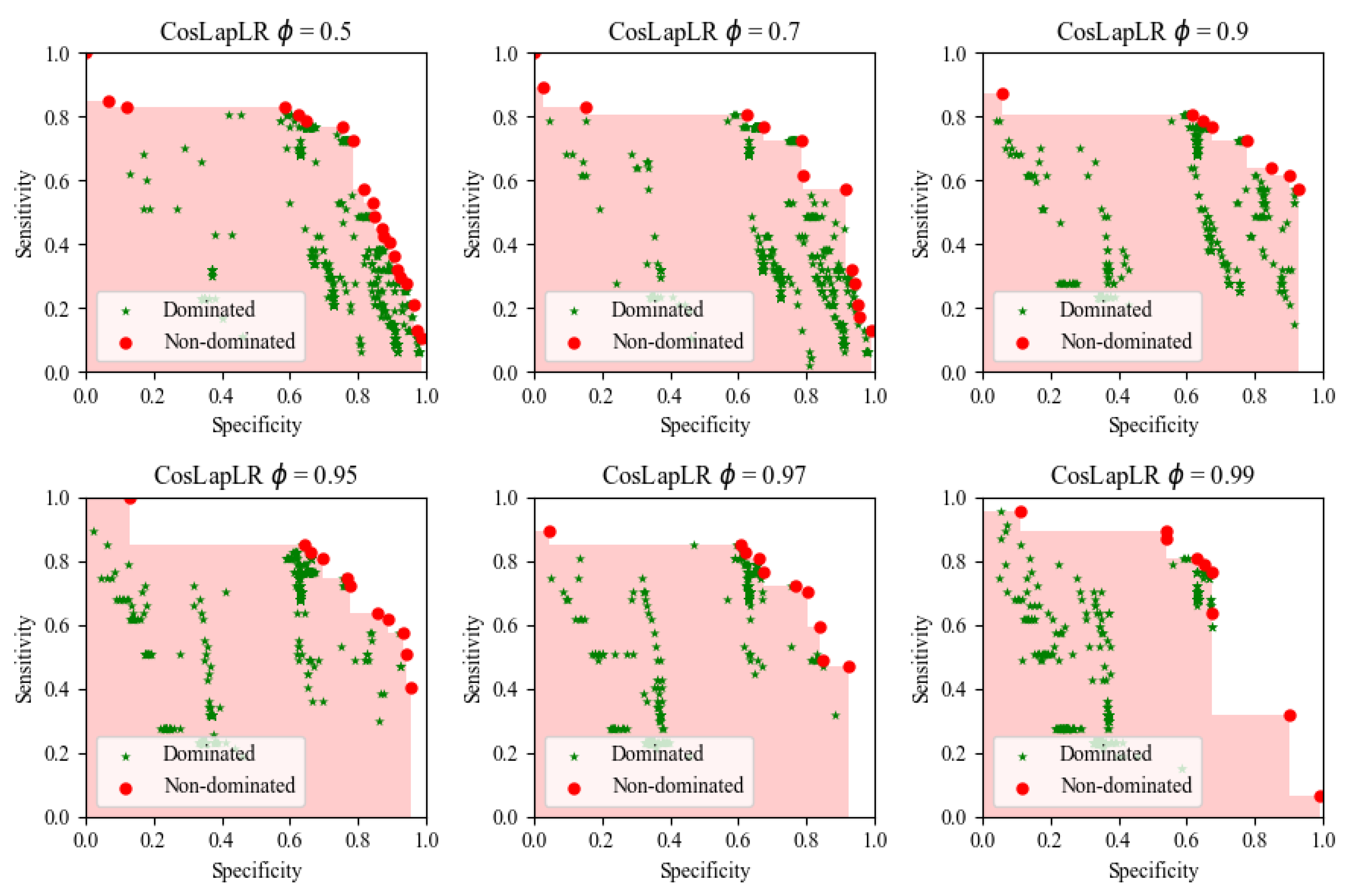
Figure 1. Pareto frontier of CosLapLR models with different cost parameter ϕ .
Mathematics 11 00119 g001
Figure 2. Pareto frontier of LR models and CosLR models.
Mathematics 11 00119 g002
Figure 3. Pareto frontier of LR models and LapLR models.
Mathematics 11 00119 g003
Table 1. Literature on ship risk prediction.
LiteraturePrediction TargetPrediction MethodData ImbalanceUnlabeled Data
Xu et al. [25,26]Ship deficiency numberSVM 1 No
Gao et al. [27]Ship deficiency numberkNN and SVMNo
Wang et al. [28]Ship deficiency numberTANNo
Chung et al. [29] and Yan et al. [30]The type and sequence of inspected deficiency codesAprioriNo
Yan et al. [31]Ship deficiency numberRandom forestNo
Yan et al. [32]Ship deficiency numberXgboostNo
Cariou and Wolff [35]Ship detention outcomeQuantile regressionNoNo
Yang et al. [42]Ship detention outcomeBNNoNo
Tsou [39]Ship detention outcomeAssociation rule mining techniquesNoNo
Wu et al. [34]Ship detention outcomeSVMNoNo
Yan et al. [3]Ship detention outcomeBRFYesNo
Our workShip detention outcomeCost-sensitive Laplacian logistic regressionYesYes
1 –: Not applicable.
Table 2. Prediction performance of binary classification models.
ϕ Modelk γ λ h λ g TN   1 FP   1 FN   1 TP   1 acc   1 spe   1 sen   1 DL   1
0.5LR25553259190.6320.6310.679167.00
LapLR332 2 13 2 7 5912896220.6750.6720.786147.50
0.7CosLR1/25553259190.6320.6310.679103.80
CosLapLR78 2 7 2 5 5912896220.6750.6720.78690.90
0.9CosLR 2 5 5543268200.6320.6300.71439.80
CosLapLR332 2 7 2 3 5703106220.6520.6480.78636.40
0.95CosLR 2 13 5832975230.6670.6630.82119.60
CosLapLR72 2 13 2 17 5822985230.6660.6610.82119.65
0.97CosLR 2 13 5763046220.6590.6550.78614.94
CosLapLR732 2 13 2 7 5812995230.6650.6600.82113.82
0.99CosLR 2 13 5753056220.6570.6530.7868.99
CosLapLR332 2 13 2 5 5543265230.6350.6300.8218.21
1TN: true negative; FP: false positive; FN: false negative; TP: true positive; acc: accuracy; spe: specificity; sen: sensitivity; DL: decision loss.
Disclaimer/Publisher’s Note: The statements, opinions and data contained in all publications are solely those of the individual author(s) and contributor(s) and not of MDPI and/or the editor(s). MDPI and/or the editor(s) disclaim responsibility for any injury to people or property resulting from any ideas, methods, instructions or products referred to in the content.