Heterogeneous Feature Fusion Module Based on CNN and Transformer for Multiview Stereo Reconstruction

Abstract

For decades, a vital area of computer vision research has been multiview stereo (MVS), which creates 3D models of a scene using photographs. This study presents an effective MVS network for 3D reconstruction utilizing multiview pictures. Alternative learning-based reconstruction techniques work well, because CNNs (convolutional neural network) can extract only the image’s local features; however, they contain many artifacts. Herein, a transformer and CNN are used to extract the global and local features of the image, respectively. Additionally, hierarchical aggregation and heterogeneous interaction modules were used to improve these features. They are based on the transformer and can extract dense features with 3D consistency and global context that are necessary to provide accurate matching for MVS.

1. Introduction

Multiview stereo (MVS) is a key technology for numerous applications, such as virtual reality, autonomous driving, and heritage preservation, which is intended to build 3D dense models of real-world situations from various photographs. Compared with other studies [1,2,3,4], recent deep learning-based approaches [5,6,7,8,9] have achieved higher accuracy and completeness on many MVS benchmarks by introducing convolutional neural networks (CNNs), indicating that deep learning is significantly more effective for feature extraction and cost volume regularization. However, the learning-based approach in MVS has many challenges. Owing to the limitations of the CNN structure, CNNs generally use fixed perceptual fields, thereby complicating the handling of texture-free surfaces while extracting image features, which limits the completeness of 3D reconstruction [10].

The computational cost of MVS, a 3D reconstruction method based on 2D pictures, is high. The following is the general definition of this task: MVS estimates the depth map of each image in a set of calibrated photographs of the same scene before reconstructing its dense point cloud. This definition has been used in most previous studies [1,2]. Recently, the prediction of depth maps in MVS has mostly relied on deep learning networks, especially CNN networks [5,6]. Such a network usually comprises the following three main components: a feature extraction network, cost volume constructor, and cost volume regularization network [10]. For the feature extraction network of MVS, most approaches use generic CNN backbone methods, such as AACVP [11], which simply superimposes a transformer network onto a CNN network to optimize the feature extraction network. Additionally, D2HRMVSNet [9] applies multiscale features for feature extraction.

Current CNN-based MVS methods usually have difficulty in handling thin structures or textureless surfaces when extracting features due to the limitation of the fixed perceptual field of CNN, which limits the robustness and integrity of 3D reconstruction [12]. Some recent studies [9,13] have improved the MVS network by using multiple scales, but the various amounts of texture information in different regions still cannot be fully utilized by multi-scale information. To solve the above problems, we compared the feature extraction components of various computer vision tasks for feature extraction in MVS. For example, for an image classification task that assigns a label to each image, global features are more important, because the entire image must be perceived as a whole. For an object detection task, local features are more important compared to global features. Semi-global feature extraction is the best match for MVS feature extraction [14] because, for high-frequency regions of the image, i.e., texture-rich regions, using local feature extraction can effectively extract features. However, for regions that are not rich in texture information, global features must be extracted. Most approaches use a general CNN backbone approach to extract features; however, owing to the limitations of CNN, CNN-based networks cannot extract global features effectively [15]. Recently, transformers have been widely used in computer vision owing to their excellent feature extraction performance; they can effectively extract global features owing to the self-attention mechanism [16].

Motivated by the aforementioned facts, we propose a novel approach to improve model performance by combining the advantages of the transformer and CNN. Generally, the CNN branch maintains local information, whereas the transformer branch simulates long-range correlations. We believe that combining these two features makes it possible to extract features for reconstruction more precisely. The following section summarizes our significant contributions:

• This study uses the parallel structure of the CNN and transformer, which is experimentally shown to extract local and global features more effectively compared to the series structure.
• We propose a feature fusion model for feature enhancement to effectively fuse the features of the CNN and transformer.
• Numerous experiments have confirmed that the proposed method outperforms other methods on the DTU dataset.

2. Related Work

2.1. Traditional MVS

MVS is a computationally expensive image-based 3D reconstruction process. In the traditional 3D reconstruction workflow of the MVS method, a sparse point cloud [17] is initially generated using a structure from motion (SfM) computation [18,19]. Thereafter, the intrinsic and extrinsic camera properties of each picture are utilized as inputs for reconstructing the dense point cloud from the sparse point cloud acquired by SfM or Simultaneous localization and mapping (SLAM). Both CMVS [20] and PMVS [21] are dense point-cloud reconstruction methods. CMVS performs 3D reconstruction using filters to filter and merge the feature points extracted by the SFM to merge the input images into a series of image clusters. Contrarily, PMVS uses clustered images from CMVS as input to generate a denser point cloud by matching and filtering features.

Although the aforementioned study produced more accurate results, high-quality results cannot be achieved for non-Lambertian surfaces, low-textured regions, and untextured regions. Therefore, the conventional MVS can be potentially improved to obtain more refined reconstruction results [10].

2.2. Learning-Based MVS

A typical MVS network comprises three main components: a feature extraction network, cost volume constructor, and cost volume regularization network. The investigation of feature extraction for MVS is currently ongoing, and most approaches use conventional CNN methods to extract the features [10]. All cost volumes must be unified in the cost volume construction module. DPSNet [22] built cost volumes by adding and aggregating all cost volumes in a principle that considers all views equally. However, because occlusion usually occurs in MVS and produces incorrect matching, creating cost volumes with equal views will result in poor prediction. Therefore, views near the reference are less likely to be obscured and should be prioritized while building the cost volume [10]. To solve this problem, gated convolution was employed using PVA-MVSNet [13] for self-adaptive aggregation of cost volumes. AA-RMVS [12] introduced an intra-view feature aggregation module to aggregate the cost volumes. The main differences between the different methods of cost volume regularization of current MVS networks can be divided into the following three main types [10]: 3D CNN, RNN, and coarse to fine, as shown in Table 1. 3D CNN is the original choice for cost volume regularization. The first MVS system built on deep learning, MVSNet [5], uses 3D U-Net to regularize cost volume. Similar to the 2D U-Net [23], the 3D U-Net features an encoder that down samples the 3D convolution and a decoder that gradually recovers the original feature resolution. However, 3D CNN requires huge computation and high memory cost, which limits the size of depth values. Furthermore, a high memory cost is necessary for dense and fine point clouds. To overcome this issue, various studies [6,9] used 2D CNN to replace 3D CNN based on D-dimensional order and RNN to pass D-dimensional contextual information. The scalability of the MVS method is improved using recurrent regularization, as the space can be divided more finely; thus, denser point clouds can be generated. Another way to significantly reduce memory use is to predict a coarse-to-fine pattern. To create a dense point cloud prediction, Cas-MVSNet [24] first created a rough depth map, which was then continuously refined. Although they focus on different contexts, the RNN and coarse-to-fine regularization algorithms offer finer depth segmentation. Larger D and more hypothetical depth planes are made possible by RNN regularization, and an adaptive depth interval subdivision for finer predictions is facilitated by coarse-to-fine regularization, which enhances the capacity to create fine details.

Table 1. Classification of learning-based MVS methods regularization scheme.

Model	Regularization Scheme
	3D CNN	RNN	Coarse to Fine
MVSNet [5]	√
R-MVSNet [6]		√
Cas-MVSNet [24]			√
CVP-MVSNet [25]			√
UCS-Net [26]			√
Vis-MVSNet [27]			√
PVA-MVSNet [13]	√
D2HC-RMVSNet [9]		√
AA-RMVSNet [12]		√

The major challenge of the MVS method is feature extraction, and most of the literature introduces CNNs for feature extraction and uses coarse-to-fine strategies for optimization. However, CNNs and coarse-to-fine techniques have difficulty capturing remote dependencies and do not effectively collect crucial data for deep inference applications [12]. To address and overcome these problems, we use a CNN with fused features retrieved by a self-attentive mechanism in the deep inference process to enhance the standard and general accuracy of the reconstructed 3D reconstruction. Additionally, we employed an RNN-based method for cost regularization; it reduces memory use and computational demands.

3. Methodology

This section details the architecture of the proposed network. Our approach draws on previous MVS methods and proposes a novel feature extraction method. Figure 1 depicts the entire system. The majority of learning-based MVS techniques are derived from MVSNet [5], which builds a beautiful and effective pipeline to determine the depth D for each input picture I, as described in the following sections.

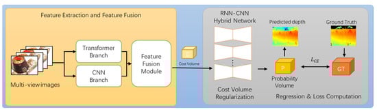
Figure 1. Overview of proposed method.

3.1. Overview of Our Method

As shown in Figure 1, the proposed general architecture follows the typical method of learning-based MVS, i.e., MVSNet, which is divided into the following three parts: a feature extraction network, described in Section 3.1; cost volume construction, described in Section 3.2; and cost regularization, described in Section 3.3.

Specifically, given $N$ images obtained from different viewpoints in a scene, all images in this study are denoted as$I_0\in R^{H\times W}$, where $H$ and $W$ correspond to the height and width of the images, respectively. Let ${\left\{I_i\right\}}_{i=1}^N$ denote the $N$ source images used as the input for reconstruction and the features ${\{F_i\in {ℝ}^{C\times H\times W}\}}_{i=1}^M$ of the input images${\left\{I_i\right\}}_{i=1}^N$, where $H$ and $W$ denote the height and width of the features, respectively, and $C$ denotes the number of channels extracted using the proposed CNN and transformer networks. In the learning-based MVS approach, the plane-sweeping technique is used to create the cost volume [10], and the entire scene was partitioned into depth spaces of M layers. Assume that ${\{d_i\in {ℝ}^{H\times W}\}}_{i=1}^M$ denotes the depth space of $M$ layers, where $d_1$ and $d_M$ denote the minimum and maximum depths, respectively. The feature volume can be constructed in a 3D space with respect to the corresponding camera parameters and differentiable homography. The homography of the feature map of the $i$th view at depth $d$ with respect to the feature map is expressed as:

$$H_i^{\left(d\right)}=d{K}_i{T}_i{T}_{ref}^{-1}{K}_{ref}^{-1}$$

(1)

where $K$ and $T$ are the intrinsic and extrinsic parameters of the camera, respectively. The cost volume for each view can then be calculated using the following formula:

$$c_i^{\left(d\right)}={\left(f_{sr{c}_i}^{\left(d\right)}-f_{ref}\right)}^2$$

(2)

where $f_{sr{c}_i}^d$ denotes the extracted features of the $i\mathrm{th}$source image, and$f_{ref}$denotes the features of the reference image. The depth map and accompanying probability distribution are then generated by performing cost volume regularization after aggregating all $N$-1 cost volumes. Therefore, we believe that image features affect the quality of cost volumes. Hence, we introduce a CNN with fused features extracted using a self-attentive mechanism into the process of deep inference to improve the quality and overall accuracy of the 3D reconstruction.

3.2. Feature Extraction Net

To use the global and local features of the input images, we propose feature extraction and feature fusion modules consisting of three sub-modules. Figure 2 depicts the trans-former branch, CNN branch, and feature fusion module.

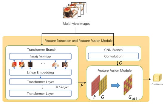
Figure 2. Overview of feature extraction net.

3.2.1. Feature Extraction Backbone Network

In this study, we propose using local and long-range correlations by extracting picture characteristics using an encoder comprising transformer branches and lightweight CNN branches.

After the transformer branch uses the patch partition module to divide the input image into non-overlapping patches, linear embedding delivers the position information and image data into the transformer layer. Thereafter, six transformer layers were applied to extract the features, as shown in Figure 3, with each layer starting with a multihead self-attention (MSA) module and ending with a multilayer perceptron (MLP). Prior to MSA and MLP, layer norm (LN) was applied, and residual connections were employed for each module. Thus, the process at level $l$ can be expressed as follows:

$${\widehat{z}}^l=MSA\left(LN\left(z^{l-1}\right)\right)+z^{l-1}$$

(3)

$$z^l=MSA\left(LN\left({\widehat{z}}^l\right)\right)+{\widehat{z}}^l$$

(4)

where ${\widehat{z}}^l$ and $z^l$ denote the MSA and MLP output features at layer $l$, respectively.

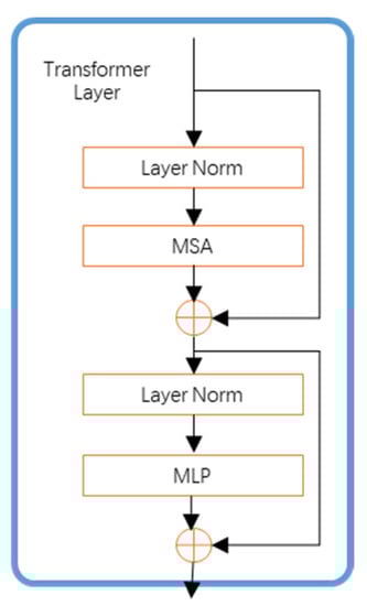
Figure 3. Feature extraction transformer part.

Similar to the vision transformer [14], we use the $N$ feature maps produced by the chosen transformer layers. After sampling and reorganization of the transformer, the desired feature maps are obtained, denoted by $F={\left\{f^n\right\}}_{n=1}^N$.

The convolution branch extracts the local information using the ResNet encoder. Herein, we employ only three ResNet convolutional layers to extract local features more effectively and avoid low-level information from being washed out by subsequent multiplications [13]. The computation time is significantly reduced, while the local features are effectively extracted. Herein, $G\in {ℝ}^{C_g\times H_g\times W_g}$ denotes the extracted local features.

Contrary to the previous MVS networks, the global features $F$ are extracted by the transformer, and local features $G$ are extracted by the convolutional network, which are fed into the feature fusion module for the next processing step.

3.2.2. Feature Fusion Module

To effectively aggregate local and global features, we use the set-to-set approach to aggregate the Transformer and CNN features using similar Depthfomer structure [13], as shown in Figure 4.

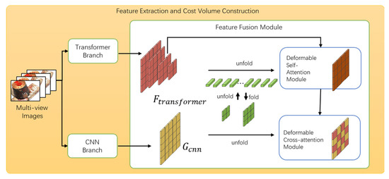
Figure 4. Overview of feature fusion part.

Specifically, the layered features of all global variables $F$ are projected onto the same channel using a 1 × 1 convolution denoted by $F_h$ that are converted into a two-dimensional matrix $X$, where each row is a $C_h$ dimensional feature vector of one pixel from the hierarchical features. Thereafter, $Q$ (query), $K$ (key), and $V$ (value) are computed using the linear projections of $X$, as follows:

$$Q=X{P}_Q,K=X{P}_K,V=X{P}_V$$

(5)

where each projection ($P_Q$, $P_K$, and $P_V$) is linear.

Self-attentive modules can also be used for feature enhancement; however, because a large number of feature vectors is required and its large memory cost is similar to that of Depthformer [13], we use the variable attention module to augment the feature vector. Let q and v index an element with representation features $x_q\in Q$ and $x_v\in V$. The position of the query vector is represented by $p_q$, and the procedure can be described as follows:

$$DAttn\left(x_q,x_v,p_q\right)={\displaystyle \sum }_{k\in {\mathsf{\Omega }}_k}{A}_{qk}·x_v\left(p_q+\Delta p_{qk}\right)$$

(6)

where the query feature $x_q$ is projected linearly across the $k^{th}$ sample point, yielding the attention weight $A_{qk}$ and sampling offset $\Delta p_{qk}$, which are $A_{qk}$ normalized as ${\displaystyle \sum }_{k\in {\mathsf{\Omega }}_k}{A}_{qk}=1$. Bilinear interpolation is used, as in [10], to obtain $x_v\left(p_q+\Delta p_{qk}\right)$, because $p_q+\Delta p_{qk}$ is a fraction. To specify which feature level each query pixel belongs to, we additionally include a hierarchical embedding. To obtain hierarchically improved features $F_{enh}$, the output $\widehat{X}$ is folded to the original resolution. We achieved feature improvement by combining $F_{enh}$ and $F$ by utilizing channel-wise concatenations and 1 × 1 convolutions to produce the result $F_0={\left\{f_0^n\right\}}_{n=1}^N$.

For local feature $G$, similar to the processing of global features $F$, we use a 1 × 1 convolution to project $G$ onto features $G_h$ having the same channel dimension $C_h$ as $F$. Thereafter, $G_h$ is spread into a 2D query matrix $Q$. Applying $X$ to $K$ and $V$, the features are aggregated using variable attention modules to minimize memory costs. The reference point position $p_q$ is dynamically predicted using a linear projection. After aggregating the $F$ and $G$, the result was reshaped to the original resolution, represented as $G_{att}$. This process achieves heterogeneous feature fusion between the transformer and CNN.

3.3. Cost Volume Construction

Since improving the cost volume regularization is tedious, we use the inter-view AA method of AA-RMVSNet [12] to match the cost volumes of all views as follows:

$$C^d=\frac{1}{N-1}{\displaystyle \sum }_{i=1}^{N-1}\left[1+\omega \left(c_i^{\left(d\right)}\right)\right]\odot c_i^{\left(d\right)}$$

(7)

where ω(·) represents adaptively generated pixel-wise attention mappings based on per-view cost volumes and ⨀ stands for Hadamard multiplication. Herein, pixels that might potentially confuse matching are muted, whereas pixels that provide important context information are given heavier weights. Compared to ω(·), 1 + ω(·) avoids over smoothness.

3.4. Cost Regularization

We used a hybrid RNN-CNN of AA-RMVSNet for cost volume regularization, during which spatial contextual information was used to generate probability distributions in depth space. The regularization network, which employs a hybrid RNN–CNN methodology, slices a cost volume ($H\times W\times D\times 32$) at dimension $D$ and simultaneously performs feature transfer along the horizontal and vertical directions. For each horizontal cost volume slice, regularization was performed using a CNN network with an encoder–decoder structure. Five parallel RNNs were employed to transport intermediate outputs from the early ConvLSTMCells to later ones in the vertical direction.

3.5. Loss Function

Most MVS networks use soft argmin [28] for the depth output, which can be interpreted as the expectation value along the depth direction [5]. The expectation formula is valid if the depth values are sampled uniformly over the depth range. However, for recurrent neural network structures, it is necessary to apply the inverse deepening method to sample the depth values to ensure a larger range of depth estimates. Instead of considering the problem as a regression task, we trained the network as a multiclass classification problem with cross-entropy loss [6]:

$$L={\displaystyle \sum }_{p\in \left\{p_v\right\}}{\displaystyle \sum }_{d=d_0}^{d_{D-1}}-G^{\left(d\right)}\left(p\right)\log \left[P^{\left(d\right)}\left(p\right)\right],$$

(8)

where $G^{\left(d\right)}\left(p\right)$ and $P^{\left(d\right)}\left(p\right)$ represent the anticipated and ground truth probabilities, respectively, of depth $d$ at pixel $p$. The collection of dependable and valid pixels is denoted as $\left\{p_v\right\}$.

4. Experiment

4.1. Dataset

A fixed camera trajectory and well-controlled laboratory settings were required to capture the indoor MVS dataset, known as DTU [29]. The dataset consisted of 79 training scans, 18 validation scans, and 22 evaluation scans out of the 128 images with 49 viewpoints obtained for 7 different lighting situations. The total number of training samples when each image was used as a reference was 27,097. For network training and assessment, we used the DTU dataset in accordance with conventional setups [5].

4.2. Implementation Details

Training: To test the proposed methodology, the DTU training set [29] was used. Similar to other previous MVS methods [5,6], because the DTU dataset contains ground truth point clouds, we first used the Poisson surface re-construction algorithm [30] and used depth rendering to create the ground truth depth maps needed for training the network. The depth maps were cross-filtered with their neighboring views using a method similar to that in [7] to increase the dependability of the original depth maps. We enlarged the original photos to have the same dimensions as the improved ground-truth depth maps, or W × H = 224 × 224. The number M of depth hypotheses evenly sampled from 425 to 935 mm was set to 100, and the number of input photos, N, was set to 7. The proposed network was trained end-to-end using Adam [31] with an initial learning rate of 0.001, which decays by 0.9 per epoch. PyTorch [32] was used to implement the proposed technique in a Linux operating system. The entire training phase takes approximately 5 days and consumes 10.16 GB of memory. For the two NVIDIA TITAN RTX GPUs, the batch size was set to 2.

Testing: The approach’s testing stage uses relatively little memory and can handle better quality images and finer depth plane sweeps; however, more memory is needed in the training phase because backpropagation is recorded to regain the intermediate gradients. In the testing phase, we generated depth maps with more accurate information, using N = 7 and M = 100.

Filtering and Fusion: We provide photometric and geometric restrictions for depth-map filtering that are comparable to earlier MVS methods. The photometric constraint employs depth, with a low confidence value, as an outlier to assess the efficacy of multiview matching. In our tests, pixels were eliminated if the computed depth probability was <0.3. In addition, we evaluated the depth consistency in multiview images using geometric constraints that remove depths that are inconsistent with their neighboring views.

4.3. Experimental Results

As listed in Table 2, we used the official MATLAB evaluation criteria provided by DTU [29] to perform the evaluation.

Table 2. Quantitative results on DTU evaluation dataset (lower is better).

Model	Acc.	Comp	O.A.
Furu [1]	0.613	0.941	0.777
Gipuma [2]	0.283	0.873	0.587
COLMAP [3]	0.400	0.664	0.532
MVSNet [5]	0.396	0.527	0.462
R-MVSNet [6]	0.385	0.459	0.422
P-MVSNet [33]	0.406	0.434	0.420
D2HC-RMVSNet [9]	0.395	0.378	0.386
PointMVSNet [34]	0.342	0.411	0.376
Vis-MVSNet [27]	0.369	0.361	0.365
Cas-MVSNet [24]	0.325	0.385	0.355
CVP-MVSNet [25]	0.296	0.406	0.351
AA-RMVSNet [12]	0.376	0.339	0.357
IterMVS [35]	0.373	0.354	0.363
EMO-MVS [36]	0.360	0.328	0.344
MVS2D [37]	0.394	0.290	0.342
Our	0.292	0.385	0.338

We calculated the mean accuracy, mean completeness, and overall accuracy to statistically assess the 3D reconstruction performance of the DTU dataset (abbreviated as OA).

$$OA=\frac{Acc.+Comp.}{2}$$

(9)

The table shows that our proposed technique performs better than other methods in terms of accuracy, overall accuracy, and completeness.

Figure 5 shows the results of comparing the reconstructed point cloud with that of GT by color. The top column of Figure 5 shows the reconstructed point cloud using the multiview image, and the bottom column shows the visualized image after comparing the reconstructed point cloud with that of GT, where the color transition from blue to red indicates the error from low to high.

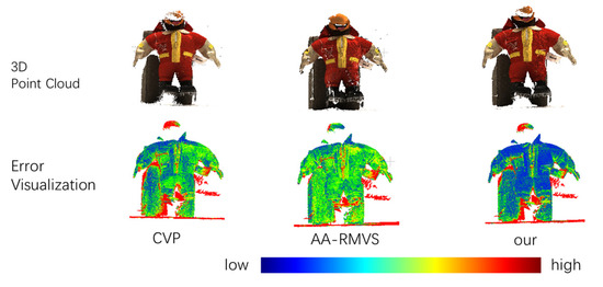
Figure 5. Error Visualization of DTU Dataset.

In Figure 6, we compare different networks to generate point cloud results. As shown in the figure, both methods improved the accuracy and completeness of the 3D reconstruction results.

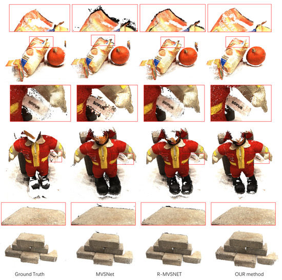
Figure 6. Comparison of 3D point cloud.

4.4. Ablation Study

This section includes ablation experiments to quantitatively assess the efficacy and dependability of the proposed feature extraction and feature aggregation methods. Based on the DTU dataset, the following tests were performed using the same parameters as in Section 4.2. The proposed method extracts global and local features using a transformer and CNN, respectively, and fuses heterogeneous features using the feature fusion module. Therefore, for a valid comparison, we use the following four different structures of feature extraction networks for the comparison experiments, as shown in Figure 7: CNN (baseline), CNN + Trans (series), CNN + Trans (parallel), and CNN + Trans + Fusion. CNN (baseline) denotes that only the CNN network is used to extract features, and the transformer network and feature CNN + Trans (series) indicate initially using the CNN network for feature extraction and then feeding the extracted features into the transformer network to obtain the final features. CNN + Trans + Fusion uses a CNN and transformer separately for feature extraction and then uses the proposed feature fusion module for feature fusion to obtain the final features.

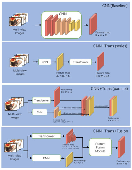
Figure 7. Schematic diagram of the ablation study network framework.

Table 3 indicates that the CNN + Trans + Fusion method is better than the other methods in terms of accuracy and overall accuracy, but slightly worse than CNN + Trans (parallel) in terms of accuracy. CNN + Trans (parallel) is better than other methods in completeness, but slightly worse in accuracy and overall accuracy and better than CNN + Trans (series). Therefore, using the transformer network in parallel with CNN can effectively improve the completeness of reconstruction. Furthermore, after adding the feature fusion module, the completeness is effectively improved, and the accuracy and overall accuracy are substantially improved compared with the baseline network.

Table 3. Quantitative results with different components on DTU evaluation dataset (lower is better).

Model	Acc.	Comp	Overall
CNN (Baseline)	0.416	0.427	0.421
CNN + Trans (series)	2.525	6.740	4.623
CNN + Trans (parallel)	0.567	0.307	0.437
CNN + Trans + Fusion	0.292	0.385	0.338
MVSNet	0.396	0.527	0.462
R-MVSNet	0.385	0.459	0.422

4.5. Complexity and Computational Efficiency

The complexity of the learning-based MVS method is usually $O\left(H\times W\times D\right)$ [5,38], but the memory requirement of the Recurrent neural network based on the number of depth samples D is independent, so the complexity is $O\left(H\times W\right)$ [6,38]. Due to the feature extraction module, the memory consumed by the network proposed in this paper is different from RMVSNET [6], but the space complexity is the same. Concerning computational efficiency, the network proposed in this paper can generate depth maps at a rate of 0.85s/view. The speed of generating depth maps here is related to refinement iterations and input image size. As shown in Table 4, param represents the number of parameters in the network, time represents the running time required to infer an image, memory represents the GPU memory required to load our network, and complexity represents the complexity of our network. We calculate the parameters and memory with the library [39]. This library is a lightweight neural network analyzer based on PyTorch [32].

Table 4. Complexity and computational efficiency.

	Param	Time	Memory	Complexity
Ours	952 K	0.85 s	4.21 GB	$O{\left(H\times W\right)}_{}$

References

- Campbell ND, F.; Vogiatzis, G.; Hernández, C.; Cipolla, R. Using multiple hypotheses to improve depth-maps for multi-view stereo. In Proceedings of the European Conference on Computer Vision, Marseille, France, 12–18 October 2008; Springer: Berlin/Heidelberg, Germany, 2008; pp. 766–779. [Google Scholar]
- Galliani, S.; Lasinger, K.; Schindler, K. Massively parallel multiview stereopsis by surface normal diffusion. In Proceedings of the IEEE International Conference on Computer Vision, Santiago, Chile, 7–13 December 2015; pp. 873–881. [Google Scholar]
- Schönberger, J.L.; Zheng, E.; Frahm, J.M.; Pollefeys, M. Pixelwise view selection for unstructured multi-view stereo. In Proceedings of the European Conference on Computer Vision, Amsterdam, The Netherlands, 11–14 October 2016; Springer: Berlin/Heidelberg, Germany, 2016; pp. 501–518. [Google Scholar]
- Barnes, C.; Shechtman, E.; Finkelstein, A.; Goldman, D.B. PatchMatch: A randomized correspondence algorithm for structural image edit-ing. ACM Trans. Graph. 2009, 28, 24. [Google Scholar] [CrossRef]
- Yao, Y.; Luo, Z.; Li, S.; Fang, T.; Quan, L. Mvsnet: Depth inference for unstructured multi-view stereo. In Proceedings of the European Con-ference on Computer Vision (ECCV), Munich, Germany, 8–14 September 2018; pp. 767–783. [Google Scholar]
- Yao, Y.; Luo, Z.; Li, S.; Shen, T.; Fang, T.; Quan, L. Recurrent mvsnet for high-resolution multi-view stereo depth inference. In Proceedings of the IEEE/CVF Conference on Computer Vision and Pattern Recognition, Long Beach, CA, USA, 15–20 June 2019; pp. 5525–5534. [Google Scholar]
- Luo, K.; Guan, T.; Ju, L.; Wang, Y.; Chen, Z.; Luo, Y. Attention-aware multi-view stereo. In Proceedings of the IEEE/CVF Conference on Computer Vision and Pattern Recognition, Seattle, WA, USA, 13–19 June 2020; pp. 1590–1599. [Google Scholar]
- Zhang, J.; Yao, Y.; Li, S.; Luo, Z.; Fang, T. Visibility-aware multi-view stereo network. arXiv 2020, arXiv:2008.07928. [Google Scholar]
- Yan, J.; Wei, Z.; Yi, H.; Ding, M.; Zhang, R.; Chen, Y.; Wang, G.; Tai, Y.-W. Dense hybrid recurrent multi-view stereo net with dynamic consistency checking. In Proceedings of the European Conference on Computer Vision, Glasgow, UK, 23–28 August 2020; Springer: Berlin/Heidelberg, Germany, 2020; pp. 674–689. [Google Scholar]
- Zhu, Q.; Min, C.; Wei, Z.; Chen, Y.; Wang, G. Deep Learning for Multi-View Stereo via Plane Sweep: A Survey. arXiv 2021, arXiv:2106.15328. [Google Scholar]
- Yu, A.; Guo, W.; Liu, B.; Chen, X.; Wang, X.; Cao, X.; Jiang, B. Attention aware cost volume pyramid based multi-view stereo network for 3d reconstruction. ISPRS J. Photogramm. Remote Sens. 2021, 175, 448–460. [Google Scholar] [CrossRef]
- Wei, Z.; Zhu, Q.; Min, C.; Chen, Y.; Wang, G. Aa-rmvsnet: Adaptive aggregation recurrent multi-view stereo network. In Proceedings of the IEEE/CVF International Conference on Computer Vision, Montreal, QC, Canada, 10–17 October 2021. [Google Scholar]
- Yi, H.; Wei, Z.; Ding, M.; Zhang, R.; Chen, Y.; Wang, G.; Tai, Y.-W. Pyramid multi-view stereo net with self-adaptive view aggregation. In Proceedings of the European Conference on Computer Vision, Glasgow, UK, 23–28 August 2020; Springer: Berlin/Heidelberg, Germany, 2020. [Google Scholar]
- Hirschmuller, H. Stereo processing by semiglobal matching and mutual information. IEEE Trans. Pattern Anal. Mach. Intell. 2007, 30, 328–341. [Google Scholar] [CrossRef] [PubMed]
- Li, Z.; Chen, Z.; Liu, X.; Jiang, J. DepthFormer: Exploiting Long-Range Correlation and Local Information for Accurate Monocular Depth Estimation. arXiv 2022, arXiv:2203.14211. [Google Scholar]
- Dosovitskiy, A.; Beyer, L.; Kolesnikov, A.; Weissenborn, D.; Zhai, X.; Unterthiner, T.; Dehghani, M.; Minderer, M.; Heigold, G.; Gelly, S.; et al. An image is worth 16 × 16 words: Transformers for image recognition at scale. arXiv 2020, arXiv:2010.11929. [Google Scholar]
- Ma, Z.; Liu, S. A review of 3D reconstruction techniques in civil engineering and their applications. Adv. Eng. Inform. 2018, 37, 163–174. [Google Scholar] [CrossRef]
- Schonberger, J.L.; Jan-Michael, F. Structure-from-motion revisited. In Proceedings of the IEEE Conference on Computer Vision and Pattern Recognition, Las Vegas, NV, USA, 27–30 June 2016. [Google Scholar]
- Yang, M.-D.; Chao, C.-F.; Huang, K.-S.; Lu, L.-Y.; Chen, Y.-P. Image-based 3D scene reconstruction and exploration in augmented reality. Autom. Con-Struction 2013, 33, 48–60. [Google Scholar] [CrossRef]
- Furukawa, Y.; Curless, B.; Seitz, S.M.; Szeliski, R. Towards internet-scale multi-view stereo. In Proceedings of the 2010 IEEE Computer Society Conference on Computer Vision and Pattern Recognition, San Francisco, CA, USA, 13–18 June 2010; IEEE: Piscatway, NJ, USA, 2010. [Google Scholar]
- Furukawa, Y.; Ponce, J. Accurate dense and robust multiview stereopsis. IEEE Trans. Pattern Anal. Mach. Intell. 2009, 32, 1362–1376. [Google Scholar] [CrossRef]
- Im, S.; Jeon, H.-G.; Lin, S.; Kweon, I.S. Dpsnet: End-to-end deep plane sweep stereo. arXiv 2019, arXiv:1905.00538. [Google Scholar]
- Ronneberger, O.; Fischer, P.; Brox, T. U-net: Convolutional networks for biomedical image segmentation. In Proceedings of the International Conference on Medical Image Computing and Computer-Assisted Intervention, Munich, Germany, 5–9 October 2015; Springer: Berlin/Heidelberg, Germany, 2015. [Google Scholar]
- Gu, X.; Fan, Z.; Zhu, S.; Dai, Z.; Tan, F.; Tan, P. Cascade cost volume for high-resolution multi-view stereo and stereo matching. In Proceedings of the IEEE/CVF Conference on Computer Vision and Pattern Recognition, Seattle, WA, USA, 13–19 June 2020. [Google Scholar]
- Yang, J.; Mao, W.; Alvarez, J.M.; Liu, M. Cost volume pyramid based depth inference for multi-view stereo. In Proceedings of the IEEE/CVF Conference on Computer Vision and Pattern Recognition, Seattle, WA, USA, 13–19 June 2020. [Google Scholar]
- Mao, Y.; Liu, Z.; Li, W.; Dai, Y.; Wang, Q.; Kim, Y.-T.; Lee, H.-S. UASNet: Uncertainty adaptive sampling network for deep stereo matching. In Proceedings of the IEEE/CVF International Conference on Computer Vision, Seattle, WA, USA, 13–19 June 2020. [Google Scholar]
- Zhang, J.; Li, S.; Luo, Z.; Fang, T.; Yao, Y. Vis-MVSNet: Visibility-Aware Multi-view Stereo Network. Int. J. Comput. Vis. 2022, 1–16. [Google Scholar] [CrossRef]
- Kendall, A.; Martirosyan, H.; Dasgupta, S.; Henry, P.; Kennedy, R.; Bachrach, A.; Bry, A. End-to-end learning of geometry and context for deep stereo regression. In Proceedings of the IEEE Inter-national Conference on Computer Vision, Venice, Italy, 22–29 October 2017. [Google Scholar]
- Jensen, R.; Dahl, A.; Vogiatzis, G.; Tola, E.; Aanaes, H. Large scale multi-view stereopsis evaluation. In Proceedings of the IEEE Conference on Computer Vision and Pattern Recognition, Columbus, OH, USA, 23–28 June 2014. [Google Scholar]
- Kazhdan, M.; Hugues, H. Screened poisson surface reconstruction. ACM Trans. Graph. 2013, 32, 1–13. [Google Scholar] [CrossRef]
- Kingma, D.P.; Jimmy, B. Adam: A method for stochastic optimization. arXiv 2014, arXiv:1412.6980. [Google Scholar]
- Paszke, A.; Gross, S.; Chintala, S.; Chanan, G.; Yang, E.; DeVito, Z.; Lin, Z.; Desmaison, A.; Antiga, L.; Lerer, A. Automatic differentiation in pytorch. In Proceedings of the Neural Information Processing Systems (NIPS) 2017 Autodiff Workshop, Long Beach, CA, USA, 9 December 2017. [Google Scholar]
- Luo, K.; Guan, T.; Ju, L.; Huang, H.; Luo, Y. P-mvsnet: Learning patch-wise matching confidence aggregation for multi-view stereo. In Proceedings of the IEEE/CVF International Conference on Computer Vision, Seoul, Republic of Korea, 27 October–2 November 2019. [Google Scholar]
- Chen, R.; Han, S.; Xu, J.; Su, H. Point-based multi-view stereo network. In Proceedings of the IEEE/CVF International Conference on Computer Vision, Seoul, Republic of Korea, 27 October–2 November 2019. [Google Scholar]
- Wang, F.; Galliani, S.; Vogel, C.; Pollefeys, M. IterMVS: Iterative Probability Estimation for Efficient Multi-View Stereo. In Proceedings of the IEEE/CVF Conference on Computer Vision and Pattern Recognition, New Orleans, Louisiana, 21–24 June 2022. [Google Scholar]
- Zhou, H.; Zhao, H.; Wang, Q.; Lei, L.; Hao, G.; Xu, Y.; Ye, Z. EMO-MVS: Error-Aware Multi-Scale Iterative Variable Optimizer for Efficient Multi-View Stereo. Remote Sens. 2022, 14, 6085. [Google Scholar] [CrossRef]
- Yang, Z.; Ren, Z.; Shan, Q.; Huang, Q. Mvs2d: Efficient multi-view stereo via attention-driven 2d convolutions. In Proceedings of the IEEE/CVF Conference on Computer Vision and Pattern Recognition, New Orleans, Louisiana, 21–24 June 2022. [Google Scholar]
- Xue, Y.; Chen, J.; Wan, W.; Huang, Y.; Yu, C.; Li, T.; Bao, J. Mvscrf: Learning multi-view stereo with conditional random fields. In Proceedings of the IEEE/CVF International Conference on Computer Vision, Seoul, Republic of Korea, 27 October–2 November 2019. [Google Scholar]
- Available online: https://github.com/Swall0w/torchstat (accessed on 17 November 2022).
Disclaimer/Publisher’s Note: The statements, opinions and data contained in all publications are solely those of the individual author(s) and contributor(s) and not of MDPI and/or the editor(s). MDPI and/or the editor(s) disclaim responsibility for any injury to people or property resulting from any ideas, methods, instructions or products referred to in the content. |
© 2022 by the authors. Licensee MDPI, Basel, Switzerland. This article is an open access article distributed under the terms and conditions of the Creative Commons Attribution (CC BY) license (https://creativecommons.org/licenses/by/4.0/).