Self-Adaptive Method and Inertial Modification for Solving the Split Feasibility Problem and Fixed-Point Problem of Quasi-Nonexpansive Mapping

Abstract

The split feasibility problem (SFP) has many practical applications, which has attracted the attention of many authors. In this paper, we propose a different method to solve the SFP and the fixed-point problem involving quasi-nonexpansive mappings. We relax the conditions of the operator as well as consider the inertial iteration and the adaptive step size. For example, the convergence generated by our new method is better than that of other algorithms, and the convergence rate of our algorithm greatly improves that of previous algorithms.

1. Introduction

Since Censor et al. [1] introduced the SFP, more and more people have paid attention to this problem due to its various applications in resolving practical issues.

Throughout this paper, we suppose that $H_1$, $H_2$ are real Hilbert spaces, and C, Q are nonempty convex closed subsets of $H_1$, $H_2$, respectively. We consider $A:H_1\to H_2$ a bounded linear operator, and $A\ne 0$. The SFP can be stated in the following form [2,3,4,5,6,7,8,9]:

Find a point $q\in H_1$, such that

$$q\in C,Aq\in Q.$$

(1)

The solution for (1) is denoted by $\mathrm{SFP}(C,Q)$:

$$\mathrm{SFP}(C,Q):=\{q\in C:Aq\in Q\}.$$

(2)

We note that the $CQ$ algorithm of Byrne [2] is a very successful approach to (1), where $\left\{q_n\right\}$ is generated by the following process:

For any initial estimation as $q_1\in H_1$,

$$q_{n+1}=P_C(q_n-{\tau }_n{A}^{*}(I-P_Q)A{q}_n),\forall n\ge 1.$$

(3)

The metric projections of C, Q are $P_C$, $P_Q$, and the adjoint operator of A is $A^{*}$. We select the step size ${\tau }_n$ with ${\tau }_n\in \left(0,\frac{2}{{\parallel A\parallel }^2}\right)$. The selection of ${\tau }_n$ is dependent on the operator norm, but the calculation of the operator norm is not easy.

The use of Formula (3) to solve (1) can be further optimized. We introduce the following function:

$$f\left(q\right):=\frac{1}{2}{\parallel (I-P_Q)Aq\parallel }^2.$$

(4)

According to the above function, we can get the following equation:

$$\nabla f\left(q\right)=A^{*}(I-P_Q)Aq.$$

(5)

Therefore, (3) is also included as a particular case of a gradient projection algorithm. In order to conquer the difficulty of numerical calculation, many authors have come up with the variable step size, which does not need to calculate norms $\parallel A\parallel$. Later on, based on predecessors, López et al. [4] thought deeply and finally put forward a new variable step size sequence ${\tau }_n$, expressed in the following form:

$${\tau }_n:=\frac{{\rho }_{n}f\left(q_n\right)}{\parallel \nabla f\left(q_n\right){\parallel }^2},\forall n\ge 1,$$

(6)

where ${\rho }_n$ satisfies these conditions: the upper bound is 4, the lower bound is 0, and ${\rho }_n$ is a sequence of positive real numbers. If we select the step size (6), we do not need to know any other conditions of the norm $\parallel A\parallel$, Q, and A.

In 2019, Qin et al. [5] introduced and studied a fixed point method to solve the SFP (1). Given that $q_1\in C$, calculate the following iteration as:

$$\left\{\begin{array}{c}{y}_n=P_C((1-{\delta }_n)(q_n-{\tau }_n{A}^{*}(I-P_Q)A{q}_n)+{\delta }_{n}S{q}_n),\hfill \\ q_{n+1}={\alpha }_{n}g\left(q_n\right)+{\beta }_n{q}_n+{\gamma }_n{y}_n,n\ge 1,\hfill \end{array}\right.$$

(7)

where $g:C\to C$ is a $k-$contraction, $S:C\to C$ is a nonexpansive mapping, $\mathrm{Fix}\left(S\right)$ denotes the set of fixed points of S. $\left\{{\alpha }_n\right\}$, $\left\{{\beta }_n\right\}$, $\left\{{\gamma }_n\right\}$, $\left\{{\delta }_n\right\}$, and $\left\{{\tau }_n\right\}$ are real sequences and belong to $(0,1)$, satisfying the following:

(${\mathrm{C}}_1$)

$0<{lim\; inf}_{n\to \infty }{\beta }_n\le {lim\; sup}_{n\to \infty }{\beta }_n<1$;

(${\mathrm{C}}_2$)

${lim}_{n\to \infty }|{\tau }_n-{\tau }_{n+1}|=0$, $0<{lim\; inf}_{n\to \infty }{\tau }_n\le {lim\; sup}_{n\to \infty }{\tau }_n<\frac{2}{{\parallel A\parallel }^2}$;

(${\mathrm{C}}_3$)

${lim}_{n\to \infty }{\alpha }_n=0$, ${\sum }_{n=1}^{\infty }{\alpha }_n=\infty$;

(${\mathrm{C}}_4$)

$0<{lim\; inf}_{n\to \infty }{\delta }_n\le {lim\; sup}_{n\to \infty }{\delta }_n<1$, ${lim}_{n\to \infty }|{\delta }_n-{\delta }_{n+1}|=0$ ;

(${\mathrm{C}}_5$)

${\alpha }_n+{\beta }_n+{\gamma }_n=1$.

Then, $\left\{q_n\right\}$ converges strongly to $x^{*}\in \mathrm{Fix}\left(S\right)\cap \mathrm{SFP}(C,Q)$, and $x^{*}$ is the unique solution of the following variational inequality:

$$⟨q-x^{*},g\left(x^{*}\right)-x^{*}⟩\le 0,\forall q\in \mathrm{Fix}\left(S\right)\cap \mathrm{SFP}(C,Q).$$

In 2020, Kraikaew et al. [6] further weakened the conditions and simplified the process of proof. They showed that the sequence $\left\{q_n\right\}$ produced by (7) converges strongly to $q^{*}\in \mathrm{Fix}\left(S\right)\cap \mathrm{SFP}(C,Q)$ when the following conditions are satisfied:

(${\mathrm{C}}_1$)

${lim\; sup}_{n\to \infty }{\beta }_n<1$;

(${\mathrm{C}}_2$)

$0<{lim\; inf}_{n\to \infty }{\tau }_n\le {lim\; sup}_{n\to \infty }{\tau }_n<\frac{2}{{\parallel A\parallel }^2}$;

(${\mathrm{C}}_3$)

${lim}_{n\to \infty }{\alpha }_n=0$, ${\sum }_{n=1}^{\infty }{\alpha }_n=\infty$;

(${\mathrm{C}}_4$)

$0<{lim\; inf}_{n\to \infty }{\delta }_n\le {lim\; sup}_{n\to \infty }{\delta }_n<1$ ;

(${\mathrm{C}}_5$)

${\alpha }_n+{\beta }_n+{\gamma }_n=1$.

Based on previous works, in this paper, we further weaken the conditions and add the inertia method so that the choice of step size does not need to calculate the operator norm.

2. Preliminaries

Throughout this paper, we suppose that H is a real Hilbert space, and D is a nonempty convex closed subset of H. For sequence $\left\{q_n\right\}$, and with q in H, we use $q_n\to q$ to represent a strong convergence and $q_n\rightharpoonup q$ to represent a weak convergence. $\mathrm{Fix}\left(T\right)$ denotes the fixed points of $T:H\to H$.

The mapping $T:H\to H$ is called:

(i)

A nonexpansive mapping if $\parallel Tx-Ty\parallel \le \parallel x-y\parallel$ for any $x,y\in H$;

(ii)

A quasi-nonexpansive mapping if $\mathrm{Fix}\left(T\right)\ne \varnothing$ and $\parallel Tx-y\parallel \le \parallel x-y\parallel$ for every $x\in H$, $y\in \mathrm{Fix}\left(T\right)$;

(iii)

A firmly nonexpansive mapping if ${\parallel Tx-Ty\parallel }^2\le {\parallel x-y\parallel }^2-{\parallel (I-T)x-(I-T)y\parallel }^2$ for any $x,y\in H$;

(iv)

A $\iota -$Lipschitz continuous mapping if there is $\iota >0$ such that $\parallel Tx-Ty\parallel \le \iota \parallel x-y\parallel$ for any $x,y\in H$;

(v)

A contraction mapping if there exists $\kappa \in [0,1)$ such that $\parallel T\left(x\right)-T\left(y\right)\parallel \le \kappa \parallel x-y\parallel$, for any $x,y\in H$.

Lemma 1

([10,11]). For any $x,y\in H$, then

(1)

${\parallel x+y\parallel }^2\le {\parallel x\parallel }^2+2⟨y,x+y⟩,\forall x,y\in X$;

(2)

${\parallel tx+(1-t)y\parallel }^2={t\parallel x\parallel }^2+{(1-t)\parallel y\parallel }^2-t(1-t){\parallel x-y\parallel }^2,\forall t\in [0,1]$.

Recall that $P_D$ is the metric projection operator, that is:

$$P_{D}y:=arg\underset{x\in D}{min}{\parallel x-y\parallel }^2,y\in H.$$

Lemma 2

([12,13,14]). Given $x\in D$ and $y\in H$,

(1)

$x=P_{D}y$ is equivalent to $⟨x-y,y-z⟩\ge 0,\forall z\in D$;

(2)

$\parallel x-P_D{y\parallel }^2\le {\parallel x-y\parallel }^2-{\parallel y-P_{D}y\parallel }^2$.

From Lemma 2, we can easily prove that $I-P_D$ is firmly nonexpansive.

Lemma 3

([15]). Let $\left\{q_n\right\}$ be a non-negative number sequence, which satisfies:

$$\begin{array}{cc}\hfill q_{n+1}& \le (1-{\Gamma }_n)q_n+{\Gamma }_n{\Lambda }_n,n\ge 1,\hfill \\ \hfill q_{n+1}& \le q_n-{\Psi }_n+{\Phi }_n,n\ge 1,\hfill \end{array}$$

where $\left\{{\Gamma }_n\right\}$ is a sequence in the open interval $(0,1)$, $\left\{{\Psi }_n\right\}$ is a non-negative real sequence, $\left\{{\Lambda }_n\right\}$, $\left\{{\Phi }_n\right\}$ are two sequences on $\mathbb{R}$, satisfying the following:

(1)

${\sum }_{n=0}^{\infty }{\Gamma }_n=\infty$;

(2)

${lim}_{n\to \infty }{\Phi }_n=0$;

(3)

${lim}_{k\to \infty }{\Psi }_{n_k}=0$ implies ${lim\; sup}_{k\to \infty }{\Lambda }_{n_k}\le 0$, where $\left\{n_k\right\}$ is a subsequence of $\left\{n\right\}$.

Then, ${lim}_{n\to \infty }{q}_n=0$.

Lemma 4

([16]). Let $f\left(q\right)=\frac{1}{2}{\parallel (I-P_Q)Aq\parallel }^2$. Then $\nabla f$ is ${\parallel A\parallel }^2-$ Lipschitz continuous.

Definition 1

([17]). Let $T:H\to H$ be a nonlinear operator with $\mathrm{Fix}\left(T\right)\ne \varnothing$, I be the identity operator. If the following implication holds for $\left\{q_n\right\}\in H$:

$$q_n\rightharpoonup qand(I-T)q_n\to 0\Rightarrow q\in \mathrm{Fix}\left(T\right),$$

then we say that $I-T$ is demiclosed at zero.

It is easy to see that this implication holds for Lipschitz continuous quasi-nonexpansive mappings (see [18]).

3. Main Results

Theorem 1.

Let $S:H_1\to H_1$ be a quasi-nonexpansive mapping. Suppose that $I-S$ is demiclosed at zero, and $g:H_1\to H_1$ is a κ-contraction. In addition, let $\left\{{\alpha }_n\right\}$, $\left\{{\beta }_n\right\}$, $\left\{{\gamma }_n\right\}$, $\left\{{\delta }_n\right\}$ be sequences in $[0,1]$, satisfying the following:

$\left({\mathrm{C}}_1\right)$

${lim\; sup}_{n\to \infty }{\beta }_n<1$;

$\left({\mathrm{C}}_2\right)$

${lim}_{n\to \infty }\frac{{ϵ}_n}{{\alpha }_n}=0$;

$\left({\mathrm{C}}_3\right)$

${lim}_{n\to \infty }{\alpha }_n=0$, ${\sum }_{n=1}^{\infty }{\alpha }_n=\infty$;

$\left({\mathrm{C}}_4\right)$

$0<{lim\; inf}_{n\to \infty }{\delta }_n\le {lim\; sup}_{n\to \infty }{\delta }_n<1$;

$\left({\mathrm{C}}_5\right)$

${\alpha }_n+{\beta }_n+{\gamma }_n=1$.

For each $n\ge 1$, we can define the following constant:

$$f\left(w_n\right):=\frac{1}{2}{\parallel (I-P_Q)A{w}_n\parallel }^2,$$

(8)

so that

$$\nabla f\left(w_n\right)=A^{*}(I-P_Q)A{w}_n.$$

If $\left\{q_n\right\}$ is defined by: $q_0,q_1\in H_1$ are arbitrarily chosen, and we have the following equation:

$$\left\{\begin{array}{c}{w}_n=q_n+{\mu }_n(q_n-q_{n-1}),\hfill \\ y_n=P_C((1-{\delta }_n)(w_n-{\tau }_n{A}^{*}(I-P_Q)A{w}_n)+{\delta }_{n}S{w}_n),\hfill \\ q_{n+1}={\alpha }_{n}g\left(q_n\right)+{\beta }_n{w}_n+{\gamma }_n{y}_n,n\ge 1,\hfill \end{array}\right.$$

(9)

$${\mu }_n=\left\{\begin{array}{cc}min\left\{\mu ,\frac{{ϵ}_n}{\parallel q_n-q_{n-1}\parallel }\right\},\hfill & \mathrm{if}{q}_n\ne q_{n-1},\hfill \\ \mu ,\hfill & \mathrm{otherwise},\hfill \end{array}\right.$$

where $\mu \ge 0$, ${\tau }_n=\frac{{\rho }_{n}f\left(w_n\right)}{\parallel \nabla f\left(w_n\right){\parallel }^2}$, ${\rho }_n\in (0,4)$, and ${\rho }_n$ is a sequence of positive real numbers. If $\nabla f\left(w_n\right)=0$, then stop; otherwise, let $n:=n+1$ and go to compute the next iteration. Assuming that $\mathrm{Fix}\left(S\right)\cap \mathrm{SFP}(C,Q)\ne \varnothing$, then $\left\{q_n\right\}$ converges strongly to $x^{*}\in \mathrm{Fix}\left(S\right)\cap \mathrm{SFP}(C,Q)$, and $x^{*}$ is the unique solution of the following variational inequality:

$$⟨z^{\prime }-x^{*},g\left(x^{*}\right)-x^{*}⟩\le 0,\forall z^{\prime }\in \mathrm{Fix}\left(S\right)\cap \mathrm{SFP}(C,Q).$$

Proof. 

From Lemma 2, we know that $x^{*}$ is a solution of the following variational inequality:

$$⟨z^{\prime }-x^{*},g\left(x^{*}\right)-x^{*}⟩\le 0,\forall z^{\prime }\in \mathrm{Fix}\left(S\right)\cap \mathrm{SFP}(C,Q),$$

if and only if $x^{*}=P_{\mathrm{Fix}\left(S\right)\cap \mathrm{SFP}(C,Q)}g\left(x^{*}\right)$. Since g is contractive and $P_{\mathrm{Fix}\left(S\right)\cap \mathrm{SFP}(C,Q)}$ is nonexpansive, we know that $P_{\mathrm{Fix}\left(S\right)\cap \mathrm{SFP}(C,Q)}g$ is contractive. Hence, such $x^{*}$ exists and is unique.

First, let $p\in \mathrm{SFP}(C,Q)\cap \mathrm{Fix}\left(S\right)$. Because $p\in C$, according to Lemma 1 and Lemma 2, we find that:

$$\begin{array}{ccc}\hfill & & \parallel y_n{-p\parallel }^2\hfill \\ & =& \parallel P_C((1-{\delta }_n)(w_n-{\tau }_n{A}^{*}(I-P_Q)A{w}_n)+{\delta }_{n}S{w}_n){-p\parallel }^2\hfill \\ & \le & \parallel ((1-{\delta }_n)(w_n-{\tau }_n{A}^{*}(I-P_Q)A{w}_n)+{\delta }_{n}S{w}_n){-p\parallel }^2\hfill \\ & & -\parallel (I-P_C)((1-{\delta }_n)(w_n-{\tau }_n{A}^{*}(I-P_Q)A{w}_n)+{\delta }_{n}S{w}_n){\parallel }^2\hfill \\ & =& \parallel {\delta }_n(S{w}_n-p)+(1-{\delta }_n)(w_n-{\tau }_n{A}^{*}(I-P_Q)A{w}_n-p){\parallel }^2\hfill \\ & & -\parallel (I-P_C)((1-{\delta }_n)(w_n-{\tau }_n{A}^{*}(I-P_Q)A{w}_n)+{\delta }_{n}S{w}_n){\parallel }^2\hfill \\ & =& {\delta }_n\parallel S{w}_n{-p\parallel }^2+(1-{\delta }_n){\parallel w_n-{\tau }_n\nabla f\left(w_n\right)-p\parallel }^2\hfill \\ & & -{\delta }_n(1-{\delta }_n){\parallel S{w}_n-w_n+{\tau }_n{A}^{*}(I-P_Q)A{w}_n\parallel }^2\hfill \\ & & -\parallel (I-P_C)((1-{\delta }_n)(w_n-{\tau }_n{A}^{*}(I-P_Q)A{w}_n)+{\delta }_{n}S{w}_n){\parallel }^2\hfill \\ & \le & {\delta }_n\parallel w_n{-p\parallel }^2+(1-{\delta }_n){\parallel w_n-{\tau }_n\nabla f\left(w_n\right)-p\parallel }^2\hfill \\ & & -{\delta }_n(1-{\delta }_n){\parallel S{w}_n-w_n+{\tau }_n{A}^{*}(I-P_Q)A{w}_n\parallel }^2\hfill \\ & & -\parallel (I-P_C)((1-{\delta }_n)(w_n-{\tau }_n{A}^{*}(I-P_Q)A{w}_n)+{\delta }_{n}S{w}_n){\parallel }^2\hfill \\ & \le & {\delta }_n\parallel w_n{-p\parallel }^2+(1-{\delta }_n)(\parallel w_n{-p\parallel }^2+{\tau }_n^2{\parallel \nabla f\left(w_n\right)\parallel }^2\hfill \\ & & -2{\tau }_n⟨\nabla f\left(w_n\right),w_n-p⟩)-{\delta }_n(1-{\delta }_n){\parallel S{w}_n-w_n+{\tau }_n{A}^{*}(I-P_Q)A{w}_n\parallel }^2\hfill \\ & & -\parallel (I-P_C)((1-{\delta }_n)(w_n-{\tau }_n{A}^{*}(I-P_Q)A{w}_n)+{\delta }_{n}S{w}_n){\parallel }^2,\hfill \end{array}$$

(10)

and

$$\begin{array}{cc}\hfill & ⟨\nabla f\left(w_n\right),w_n-p⟩\hfill \\ =& ⟨(I-P_Q)A{w}_n-(I-P_Q)Ap,A{w}_n-Ap⟩\hfill \\ \ge & \parallel (I-P_Q)A{w}_n{\parallel }^2\hfill \\ =& 2f\left(w_n\right).\hfill \end{array}$$

(11)

Therefore, by combining (10) and (11), we derive the following:

$$\begin{array}{cc}\hfill & \parallel y_n{-p\parallel }^2\hfill \\ \le & \parallel w_n{-p\parallel }^2-4(1-{\delta }_n){\tau }_{n}f\left(w_n\right)+{\tau }_n^2(1-{\delta }_n){\parallel \nabla f\left(w_n\right)\parallel }^2\hfill \\ & -{\delta }_n(1-{\delta }_n){\parallel S{w}_n-w_n+{\tau }_n{A}^{*}(I-P_Q)A{w}_n\parallel }^2\hfill \\ & -\parallel (I-P_C)((1-{\delta }_n)(w_n-{\tau }_n{A}^{*}(I-P_Q)A{w}_n)+{\delta }_{n}S{w}_n){\parallel }^2\hfill \\ =& \parallel w_n{-p\parallel }^2-{\rho }_n(4-{\rho }_n)(1-{\delta }_n)\frac{f^2\left(w_n\right)}{\parallel \nabla f\left(w_n\right){\parallel }^2}\hfill \\ & -{\delta }_n(1-{\delta }_n){\parallel S{w}_n-w_n+{\tau }_n{A}^{*}(I-P_Q)A{w}_n\parallel }^2\hfill \\ & -\parallel (I-P_C)((1-{\delta }_n)(w_n-{\tau }_n{A}^{*}(I-P_Q)A{w}_n)+{\delta }_{n}S{w}_n){\parallel }^2.\hfill \end{array}$$

(12)

Note that ${\rho }_n\in (0,4)$, $\left\{{\delta }_n\right\}$ is a sequence in $(0,1)$. We thus derive the following equation:

$$\parallel y_n-p\parallel \le \parallel w_n-p\parallel .$$

(13)

Putting $z_n=\frac{{\beta }_n}{1-{\alpha }_n}{w}_n+\frac{{\gamma }_n}{1-{\alpha }_n}{y}_n$, by Lemma 1, we can derive that:

$$\begin{array}{ccc}& & \parallel z_n{-p\parallel }^2\hfill \\ & =& {∥\frac{{\beta }_n}{1-{\alpha }_n}{w}_n+\frac{{\gamma }_n}{1-{\alpha }_n}{y}_n-p∥}^2\hfill \\ & =& {∥\frac{{\beta }_n}{1-{\alpha }_n}(w_n-p)+\frac{{\gamma }_n}{1-{\alpha }_n}(y_n-p)∥}^2\hfill \\ & =& \frac{{\beta }_n}{1-{\alpha }_n}\parallel w_n{-p\parallel }^2+\frac{{\gamma }_n}{1-{\alpha }_n}\parallel y_n{-p\parallel }^2-\frac{{\beta }_n}{1-{\alpha }_n}\frac{{\gamma }_n}{1-{\alpha }_n}{\parallel w_n-y_n\parallel }^2.\hfill \end{array}$$

From the conditions imposed on $\left\{{\alpha }_n\right\}$, $\left\{{\beta }_n\right\}$, $\left\{{\gamma }_n\right\}$ and (12), we have the following:

$$\begin{array}{ccc}\hfill & & \parallel z_n{-p\parallel }^2\hfill \\ & \le & \frac{{\beta }_n}{1-{\alpha }_n}\parallel w_n{-p\parallel }^2+\frac{{\gamma }_n}{1-{\alpha }_n}{\parallel y_n-p\parallel }^2\hfill \\ & \le & \frac{{\beta }_n}{1-{\alpha }_n}\parallel w_n{-p\parallel }^2+\frac{{\gamma }_n}{1-{\alpha }_n}{\parallel w_n-p\parallel }^2\hfill \\ & & -(1-{\delta }_n)\frac{{\gamma }_n}{1-{\alpha }_n}{\rho }_n(4-{\rho }_n)\frac{f^2\left(w_n\right)}{\parallel \nabla f\left(w_n\right){\parallel }^2}\hfill \\ & & -\frac{{\gamma }_n}{1-{\alpha }_n}{\delta }_n(1-{\delta }_n){\parallel S{w}_n-w_n+{\tau }_n{A}^{*}(I-P_Q)A{w}_n\parallel }^2\hfill \\ & & -\frac{{\gamma }_n}{1-{\alpha }_n}{\parallel (I-P_C)((1-{\delta }_n)(w_n-{\tau }_n{A}^{*}(I-P_Q)A{w}_n)+{\delta }_{n}S{w}_n)\parallel }^2\hfill \\ & =& \parallel w_n{-p\parallel }^2-(1-{\delta }_n)\frac{{\gamma }_n}{1-{\alpha }_n}{\rho }_n(4-{\rho }_n)\frac{f^2\left(w_n\right)}{\parallel \nabla f\left(w_n\right){\parallel }^2}\hfill \\ & & -\frac{{\gamma }_n}{1-{\alpha }_n}{\delta }_n(1-{\delta }_n){\parallel S{w}_n-w_n+{\tau }_n{A}^{*}(I-P_Q)A{w}_n\parallel }^2\hfill \\ & & -\frac{{\gamma }_n}{1-{\alpha }_n}{\parallel (I-P_C)((1-{\delta }_n)(w_n-{\tau }_n{A}^{*}(I-P_Q)A{w}_n)+{\delta }_{n}S{w}_n)\parallel }^2.\hfill \end{array}$$

(14)

From the conditions imposed on $\left\{{\alpha }_n\right\}$, $\left\{{\delta }_n\right\}$ and $\left\{{\gamma }_n\right\}$, we have the following equation:

$$\parallel z_n-p\parallel \le \parallel w_n-p\parallel .$$

(15)

Since $z_n=\frac{{\beta }_n}{1-{\alpha }_n}{w}_n+\frac{{\gamma }_n}{1-{\alpha }_n}{y}_n$, we can get the equations below:

$$\begin{array}{ccc}\hfill q_{n+1}& =& {\alpha }_{n}g\left(q_n\right)+{\beta }_n{w}_n+{\gamma }_n{y}_n\hfill \\ & =& {\alpha }_{n}g\left(q_n\right)+(1-{\alpha }_n)z_n.\hfill \end{array}$$

Since g is a $\kappa$-contraction and by using (15), we can get the following:

$$\begin{array}{ccc}& & \parallel q_{n+1}-p\parallel \hfill \\ & =& \parallel {\alpha }_{n}g\left(q_n\right)+(1-{\alpha }_n)z_n-p\parallel \hfill \\ & =& \parallel {\alpha }_n(g\left(q_n\right)-p)+(1-{\alpha }_n)(z_n-p)\parallel \hfill \\ & \le & {\alpha }_n\parallel g\left(q_n\right)-p\parallel +(1-{\alpha }_n)\parallel z_n-p\parallel \hfill \\ & \le & {\alpha }_n\parallel g\left(q_n\right)-p\parallel +(1-{\alpha }_n)\parallel w_n-p\parallel \hfill \\ & \le & {\alpha }_n\parallel g\left(q_n\right)-g\left(p\right)\parallel +{\alpha }_n\parallel g\left(p\right)-p\parallel +(1-{\alpha }_n)\parallel q_n-p+{\mu }_n(q_n-q_{n-1})\parallel \hfill \\ & \le & {\alpha }_n\kappa \parallel q_n-p\parallel +{\alpha }_n\parallel g\left(p\right)-p\parallel +(1-{\alpha }_n)\parallel q_n-p\parallel \hfill \\ & & +(1-{\alpha }_n)\parallel {\mu }_n(q_n-q_{n-1})\parallel \hfill \\ & \le & {\alpha }_n\kappa \parallel q_n-p\parallel +{\alpha }_n\parallel g\left(p\right)-p\parallel +(1-{\alpha }_n)\parallel q_n-p\parallel +{\mu }_n\parallel q_n-q_{n-1}\parallel \hfill \\ & \le & {\alpha }_n\kappa \parallel q_n-p\parallel +{\alpha }_n\parallel g\left(p\right)-p\parallel +(1-{\alpha }_n)\parallel q_n-p\parallel +{ϵ}_n\hfill \\ & =& (1-{\alpha }_n(1-\kappa ))\parallel q_n-p\parallel +{\alpha }_n(1-\kappa )\left(\frac{\parallel g\left(p\right)-p\parallel }{1-\kappa }+\frac{{ϵ}_n}{{\alpha }_n(1-\kappa )}\right).\hfill \end{array}$$

Since ${lim}_{n\to \infty }\frac{{ϵ}_n}{{\alpha }_n}=0$, we therefore have $\frac{{ϵ}_n}{{\alpha }_n}<M$, where M is a suitable positive constant. Hence, we have the following:

$$\begin{array}{ccc}& & \parallel q_{n+1}-p\parallel \hfill \\ & \le & (1-{\alpha }_n(1-\kappa ))\parallel q_n-p\parallel +{\alpha }_n(1-\kappa )\left(\frac{\parallel g\left(p\right)-p\parallel +M}{1-\kappa }\right)\hfill \\ & \le & max\left\{\parallel q_n-p\parallel ,\frac{\parallel g\left(p\right)-p\parallel +M}{1-\kappa }\right\}\hfill \end{array}$$

We can thus deduce that:

$$\parallel q_{n+1}-p\parallel \le max\left\{\parallel q_1-p\parallel ,\frac{\parallel g\left(p\right)-p\parallel +M}{1-\kappa }\right\}.$$

(16)

Therefore, the sequence $\{\parallel q_n-p\parallel \}$ is bounded.

From Lemma 1, we can get the following:

$$\begin{array}{ccc}\hfill \parallel w_n{-p\parallel }^2& =& \parallel q_n+{\mu }_n(q_n-q_{n-1}){-p\parallel }^2\hfill \\ & \le & \parallel q_n{-p\parallel }^2+2{\mu }_n⟨q_n-q_{n-1},w_n-p⟩\hfill \\ & \le & \parallel q_n{-p\parallel }^2+2{\mu }_n\parallel q_n-q_{n-1}\parallel \parallel w_n-p\parallel \hfill \\ & \le & \parallel q_n{-p\parallel }^2+2{ϵ}_n\parallel w_n-p\parallel .\hfill \end{array}$$

We derive that:

$$\parallel w_n{-p\parallel }^2\le \parallel q_n{-p\parallel }^2+2{ϵ}_n\parallel w_n-p\parallel .$$

(17)

As p is chosen arbitrarily and g is a $\kappa$-contraction, we have the following equations:

$$\begin{array}{ccc}\hfill & & \parallel q_{n+1}-x^{*}{\parallel }^2\hfill \\ & =& \parallel {\alpha }_{n}g\left(q_n\right)+(1-{\alpha }_n)z_n-x^{*}{\parallel }^2\hfill \\ & =& \parallel {\alpha }_n(g\left(q_n\right)-x^{*})+(1-{\alpha }_n)(z_n-x^{*}){\parallel }^2\hfill \\ & \le & {\alpha }_n^2\parallel g\left(q_n\right)-x^{*}{\parallel }^2+{(1-{\alpha }_n)}^2{\parallel z_n-x^{*}\parallel }^2\hfill \\ & & +2{\alpha }_n⟨g\left(q_n\right)-x^{*},z_n-x^{*}⟩-2{\alpha }_n^2⟨g\left(q_n\right)-x^{*},z_n-x^{*}⟩\hfill \\ & \le & {\alpha }_n^2\parallel g\left(q_n\right)-x^{*}{\parallel }^2+{(1-{\alpha }_n)}^2{\parallel z_n-x^{*}\parallel }^2\hfill \\ & & +2{\alpha }_n⟨g\left(q_n\right)-x^{*},z_n-x^{*}⟩+2{\alpha }_n^2\parallel g\left(q_n\right)-x^{*}\parallel \parallel z_n-x^{*}\parallel \hfill \\ & =& {\alpha }_n^2\parallel g\left(q_n\right)-x^{*}{\parallel }^2+{(1-{\alpha }_n)}^2{\parallel z_n-x^{*}\parallel }^2+2{\alpha }_n⟨g\left(q_n\right)-g\left(x^{*}\right),z_n-x^{*}⟩\hfill \\ & & +2{\alpha }_n⟨g\left(x^{*}\right)-x^{*},z_n-x^{*}⟩+2{\alpha }_n^2\parallel g\left(q_n\right)-x^{*}\parallel \parallel z_n-x^{*}\parallel \hfill \\ & \le & {\alpha }_n^2\parallel g\left(q_n\right)-x^{*}{\parallel }^2+{(1-{\alpha }_n)}^2\parallel z_n-x^{*}{\parallel }^2+2{\alpha }_n\kappa \parallel q_n-x^{*}\parallel \parallel z_n-x^{*}\parallel \hfill \\ & & +2{\alpha }_n⟨g\left(x^{*}\right)-x^{*},z_n-x^{*}⟩+2{\alpha }_n^2\parallel g\left(q_n\right)-x^{*}\parallel \parallel z_n-x^{*}\parallel \hfill \\ & \le & {\alpha }_n^2\parallel g\left(q_n\right)-x^{*}{\parallel }^2+2{\alpha }_n^2\parallel g\left(q_n\right)-x^{*}\parallel \parallel z_n-x^{*}\parallel +{(1-{\alpha }_n)}^2{\parallel z_n-x^{*}\parallel }^2\hfill \\ & & +{\alpha }_n\kappa (\parallel q_n-x^{*}{\parallel }^2+\parallel z_n-x^{*}{\parallel }^2)+2{\alpha }_n⟨g\left(x^{*}\right)-x^{*},z_n-x^{*}⟩.\hfill \end{array}$$

(18)

From (15) and (17), we can derive that:

$$\parallel z_n-x^{*}{\parallel }^2\le \parallel q_n-x^{*}{\parallel }^2+2{ϵ}_n\parallel w_n-x^{*}\parallel .$$

(19)

It thus follows from (18) and (19) that:

$$\begin{array}{ccc}\hfill & & \parallel q_{n+1}-x^{*}{\parallel }^2\hfill \\ & \le & {\alpha }_n^2\parallel g\left(q_n\right)-x^{*}{\parallel }^2+2{\alpha }_n^2\parallel g\left(q_n\right)-x^{*}\parallel \parallel z_n-x^{*}\parallel \hfill \\ & & +{\alpha }_n\kappa (\parallel q_n-x^{*}{\parallel }^2+\parallel q_n-x^{*}{\parallel }^2+2{ϵ}_n\parallel w_n-x^{*}\parallel )\hfill \\ & & +2{\alpha }_n⟨g\left(x^{*}\right)-x^{*},z_n-x^{*}⟩+{(1-{\alpha }_n)}^2(\parallel q_n-x^{*}{\parallel }^2+2{ϵ}_n\parallel w_n-x^{*}\parallel )\hfill \\ & =& {\alpha }_n^2\parallel g\left(q_n\right)-x^{*}{\parallel }^2+2{\alpha }_n^2\parallel g\left(q_n\right)-x^{*}\parallel \parallel z_n-x^{*}\parallel \hfill \\ & & +({\alpha }_n^2+(1-2{\alpha }_n(1-\kappa ))){\parallel q_n-x^{*}\parallel }^2\hfill \\ & & +(2{ϵ}_n{(1-{\alpha }_n)}^2+2{\alpha }_n\kappa {ϵ}_n)\parallel w_n-x^{*}\parallel +2{\alpha }_n⟨g\left(x^{*}\right)-x^{*},z_n-x^{*}⟩\hfill \\ & \le & {\alpha }_n^2\parallel g\left(q_n\right)-x^{*}{\parallel }^2+2{\alpha }_n^2\parallel g\left(q_n\right)-x^{*}\parallel \parallel z_n-x^{*}\parallel +{\alpha }_n^2{\parallel q_n-x^{*}\parallel }^2\hfill \\ & & +(1-2{\alpha }_n(1-\kappa ))\parallel q_n-x^{*}{\parallel }^2+4{ϵ}_n\parallel w_n-x^{*}\parallel +2{\alpha }_n⟨g\left(x^{*}\right)-x^{*},z_n-x^{*}⟩\hfill \\ & =& (1-2{\alpha }_n(1-\kappa ))\parallel q_n-x^{*}{\parallel }^2+{\alpha }_n({\alpha }_n{\parallel g\left(q_n\right)-x^{*}\parallel }^2\hfill \\ & & +2{\alpha }_n\parallel g\left(q_n\right)-x^{*}\parallel \parallel z_n-x^{*}\parallel +{\alpha }_n\parallel q_n-x^{*}{\parallel }^2+\frac{4{ϵ}_n}{{\alpha }_n}\parallel w_n-x^{*}\parallel \hfill \\ & & +2⟨g\left(x^{*}\right)-x^{*},z_n-x^{*}⟩)\hfill \\ & =& (1-2{\alpha }_n(1-\kappa ))\parallel q_n-x^{*}{\parallel }^2+2{\alpha }_n(1-\kappa )\frac{1}{2(1-\kappa )}({\alpha }_n{\parallel g\left(q_n\right)-x^{*}\parallel }^2\hfill \\ & & +2{\alpha }_n\parallel g\left(q_n\right)-x^{*}\parallel \parallel z_n-x^{*}\parallel +{\alpha }_n{\parallel q_n-x^{*}\parallel }^2\hfill \\ & & +\frac{4{ϵ}_n}{{\alpha }_n}\parallel w_n-x^{*}\parallel +2⟨g\left(x^{*}\right)-x^{*},z_n-x^{*}⟩).\hfill \end{array}$$

(20)

On the other hand, by Lemma 1, we can derive that:

$$\begin{array}{ccc}\hfill & & \parallel q_{n+1}-x^{*}{\parallel }^2\hfill \\ & =& \parallel {\alpha }_n(g\left(q_n\right)-z_n)+z_n-x^{*}{\parallel }^2\hfill \\ & \le & \parallel z_n-x^{*}{\parallel }^2+2{\alpha }_n⟨g\left(x_n\right)-z_n,x_{n+1}-x^{*}⟩.\hfill \end{array}$$

(21)

From (14), (17), (21), we find the following:

$$\begin{array}{ccc}& & \parallel q_{n+1}-x^{*}{\parallel }^2\hfill \\ & \le & \parallel w_n-x^{*}{\parallel }^2-(1-{\delta }_n)\frac{{\gamma }_n}{1-{\alpha }_n}{\rho }_n(4-{\rho }_n)\frac{f^2\left(w_n\right)}{\parallel \nabla f\left(w_n\right){\parallel }^2}\hfill \\ & & -\frac{{\gamma }_n}{1-{\alpha }_n}{\delta }_n(1-{\delta }_n){\parallel S{w}_n-w_n+{\tau }_n{A}^{*}(I-P_Q)A{w}_n\parallel }^2\hfill \\ & & -\frac{{\gamma }_n}{1-{\alpha }_n}\parallel (I-P_C)((1-{\delta }_n)(w_n-{\tau }_n{A}^{*}(I-P_Q)A{w}_n)\hfill \\ & & +{\delta }_{n}S{w}_n{)\parallel }^2+2{\alpha }_n⟨g\left(q_n\right)-z_n,q_{n+1}-x^{*}⟩\hfill \\ & \le & \parallel q_n-x^{*}{\parallel }^2+2{ϵ}_n\parallel w_n-x^{*}\parallel -(1-{\delta }_n)\frac{{\gamma }_n}{1-{\alpha }_n}{\rho }_n(4-{\rho }_n)\frac{f^2\left(w_n\right)}{\parallel \nabla f\left(w_n\right){\parallel }^2}\hfill \\ & & -\frac{{\gamma }_n}{1-{\alpha }_n}{\delta }_n(1-{\delta }_n){\parallel S{w}_n-w_n+{\tau }_n{A}^{*}(I-P_Q)A{w}_n\parallel }^2\hfill \\ & & -\frac{{\gamma }_n}{1-{\alpha }_n}\parallel (I-P_C)((1-{\delta }_n)(w_n-{\tau }_n{A}^{*}(I-P_Q)A{w}_n)\hfill \\ & & +{\delta }_{n}S{w}_n{)\parallel }^2+2{\alpha }_n⟨g\left(x_n\right)-z_n,q_{n+1}-x^{*}⟩.\hfill \end{array}$$

Thus,

$$\begin{array}{ccc}\hfill & & \parallel q_{n+1}-x^{*}{\parallel }^2\hfill \\ & \le & \parallel q_n-x^{*}{\parallel }^2+2{ϵ}_n\parallel w_n-x^{*}\parallel -(1-{\delta }_n)\frac{{\gamma }_n}{1-{\alpha }_n}{\rho }_n(4-{\rho }_n)\frac{f^2\left(w_n\right)}{\parallel \nabla f\left(w_n\right){\parallel }^2}\hfill \\ & & -\frac{{\gamma }_n}{1-{\alpha }_n}{\delta }_n(1-{\delta }_n){\parallel S{w}_n-w_n+{\tau }_n{A}^{*}(I-P_Q)A{w}_n\parallel }^2\hfill \\ & & -\frac{{\gamma }_n}{1-{\alpha }_n}\parallel (I-P_C)((1-{\delta }_n)(w_n-{\tau }_n{A}^{*}(I-P_Q)A{w}_n)\hfill \\ & & +{\delta }_{n}S{w}_n{)\parallel }^2+2{\alpha }_n⟨g\left(q_n\right)-z_n,q_{n+1}-x^{*}⟩.\hfill \end{array}$$

(22)

Set the following:

$$\begin{array}{ccc}\hfill {\Gamma }_n& =& 2{\alpha }_n(1-\kappa ),\hfill \\ \hfill {\Lambda }_n& =& \frac{1}{2(1-\kappa )}({\alpha }_n{\parallel g\left(q_n\right)-x^{*}\parallel }^2\hfill \\ & & +2{\alpha }_n\parallel g\left(q_n\right)-x^{*}\parallel \parallel z_n-x^{*}\parallel +{\alpha }_n{\parallel q_n-x^{*}\parallel }^2\hfill \\ & & +\frac{2{ϵ}_n}{{\alpha }_n}\parallel w_n-x^{*}\parallel +2⟨g\left(x^{*}\right)-x^{*},z_n-x^{*}⟩),\hfill \\ \hfill {\Psi }_n& =& (1-{\delta }_n)\frac{{\gamma }_n}{1-{\alpha }_n}{\rho }_n(4-{\rho }_n)\frac{f^2\left(w_n\right)}{\parallel \nabla f\left(w_n\right){\parallel }^2}\hfill \\ & & +\frac{{\gamma }_n}{1-{\alpha }_n}{\delta }_n(1-{\delta }_n){\parallel S{w}_n-w_n+{\tau }_n{A}^{*}(I-P_Q)A{w}_n\parallel }^2\hfill \\ & & +\frac{{\gamma }_n}{1-{\alpha }_n}{\parallel (I-P_C)((1-{\delta }_n)(w_n-{\tau }_n{A}^{*}(I-P_Q)A{w}_n)+{\delta }_{n}S{w}_n)\parallel }^2,\hfill \\ \hfill {\Phi }_n& =& 2{\alpha }_n⟨g\left(q_n\right)-z_n,q_{n+1}-x^{*}⟩.\hfill \end{array}$$

Then, (20) and (22) can be rewritten as follows:

$$\begin{array}{cc}\hfill \parallel q_{n+1}-x^{*}{\parallel }^2& \le (1-{\Gamma }_n){\parallel q_n-x^{*}\parallel }^2+{\Gamma }_n{\Lambda }_n,\hfill \\ \hfill \parallel q_{n+1}-x^{*}{\parallel }^2& \le \parallel q_n-x^{*}{\parallel }^2-{\Psi }_n+{\Phi }_n.\hfill \end{array}$$

It is easy to see that ${lim}_{n\to \infty }{\Gamma }_n=0$, ${\sum }_{n=0}^{\infty }{\Gamma }_n=\infty$, and ${lim}_{n\to \infty }{\Phi }_n=0$. Therefore, by Lemma 3, we prove that ${lim}_{n\to \infty }\parallel q_n-x^{*}\parallel =0$ if we show that ${lim\; sup}_{k\to \infty }{\Lambda }_{n_k}\le 0$ whenever ${lim}_{k\to \infty }{\Psi }_{n_k}=0$ for any subsequence $\left\{n_k\right\}\subset \left\{n\right\}$.

Suppose that

$$\underset{k\to \infty }{lim}{\Psi }_{n_k}=0.$$

(23)

By the conditions of $\left\{{\alpha }_n\right\}$, $\left\{{\beta }_n\right\}$, $\left\{{\delta }_n\right\}$, and $\left\{{\gamma }_n\right\}$, we have the following equations:

$$\underset{k\to \infty }{lim}{\rho }_{n_k}(4-{\rho }_{n_k})\frac{f^2\left(w_{n_k}\right)}{\parallel \nabla f\left(w_{n_k}\right){\parallel }^2}=0,$$

(24)

$$\underset{k\to \infty }{lim}{\parallel S{w}_{n_k}-w_{n_k}+{\tau }_{n_k}{A}^{*}(I-P_Q)A{w}_{n_k}\parallel }^2=0,$$

(25)

$$\underset{k\to \infty }{lim}\parallel (I-P_C)((1-{\delta }_{n_k})(w_{n_k}-{\tau }_{n_k}\nabla f\left(w_{n_k}\right))+{\delta }_{n_k}S{w}_{n_k})\parallel =0.$$

(26)

Equation (24) implies that:

$$\frac{f^2\left(w_{n_k}\right)}{\parallel \nabla f\left(w_{n_k}\right){\parallel }^2}\to 0.$$

(27)

From Lemma 4, since $\{\parallel \nabla f\left(w_{n_k}\right)\parallel \}$ is bounded, we derive that $f\left(w_{n_k}\right)\to 0$ as $k\to \infty$, so ${lim}_{k\to \infty }\parallel (I-P_Q)A{w}_{n_k}\parallel =0$. By using (27) and the conditions on $\left\{{\rho }_n\right\}$, we get the following:

$${\tau }_{n_k}\parallel \nabla f\left(w_{n_k}\right)\parallel =\frac{{\rho }_{n_k}f\left(w_{n_k}\right)}{\parallel \nabla f\left(w_{n_k}\right)\parallel }\to 0.$$

(28)

Moreover, according to (25), we can get the equation below:

$$\parallel S{w}_{n_k}-w_{n_k}\parallel \to 0.$$

(29)

From (26), by expanding the formula, since $y_{n_k}=P_C((1-{\delta }_{n_k})(w_{n_k}-{\tau }_{n_k}\nabla f\left(w_{n_k}\right))+{\delta }_{n_k}S{w}_{n_k})$, we can get:

$$\parallel (1-{\delta }_{n_k})(w_{n_k}-{\tau }_{n_k}\nabla f\left(w_{n_k}\right))+{\delta }_{n_k}S{w}_{n_k}-y_{n_k}\parallel \to 0.$$

(30)

By expanding (30), we can get the following equation:

$$\parallel (1-{\delta }_{n_k})w_{n_k}-(1-{\delta }_{n_k}){\tau }_{n_k}\nabla f\left(w_{n_k}\right)+{\delta }_{n_k}S{w}_{n_k}-y_{n_k}\parallel \to 0.$$

(31)

With (31) and (28), we can derive the equation below:

$$\parallel (1-{\delta }_{n_k})w_{n_k}+{\delta }_{n_k}S{w}_{n_k}-y_{n_k}\parallel \to 0,$$

(32)

i.e.,

$$\parallel w_{n_k}-y_{n_k}+{\delta }_{n_k}(S{w}_{n_k}-w_{n_k})\parallel \to 0.$$

(33)

Hence, we arrive at the following:

$$\begin{array}{ccc}& & \parallel w_{n_k}-y_{n_k}\parallel \hfill \\ & =& \parallel w_{n_k}-y_{n_k}+{\delta }_{n_k}(S{w}_{n_k}-w_{n_k})-{\delta }_{n_k}(S{w}_{n_k}-w_{n_k})\parallel \hfill \\ & \le & \parallel w_{n_k}-y_{n_k}+{\delta }_{n_k}(S{w}_{n_k}-w_{n_k})\parallel +\parallel {\delta }_{n_k}(S{w}_{n_k}-w_{n_k})\parallel .\hfill \end{array}$$

Then, from (29) and (33), we can derive that:

$$\parallel w_{n_k}-y_{n_k}\parallel \to 0.$$

(34)

From the definition of $z_n$, we can see the following:

$$\begin{array}{ccc}\hfill \parallel z_{n_k}-w_{n_k}\parallel & =& ∥\frac{{\beta }_{n_k}}{1-{\alpha }_{n_k}}{w}_{n_k}+\frac{{\gamma }_{n_k}}{1-{\alpha }_{n_k}}{y}_{n_k}-w_{n_k}∥\hfill \\ & =& ∥-\frac{{\gamma }_{n_k}}{1-{\alpha }_{n_k}}{w}_{n_k}+\frac{{\gamma }_{n_k}}{1-{\alpha }_{n_k}}{y}_{n_k}∥\hfill \\ & =& \frac{{\gamma }_{n_k}}{1-{\alpha }_{n_k}}\parallel y_{n_k}-w_{n_k}\parallel .\hfill \end{array}$$

By using (34), we can get the following:

$$\parallel z_{n_k}-w_{n_k}\parallel \to 0.$$

(35)

Combining (29) and the fact that $I-S$ is demiclosed at zero, we know ${\omega }_w\left(w_{n_k}\right)\subset \mathrm{Fix}\left(S\right)$. We select a subsequence $\left\{w_{n_{k_j}}\right\}$ of $\left\{w_{n_k}\right\}$ to satisfy the following equation:

$$\underset{k\to \infty }{lim\; sup}⟨g\left(x^{*}\right)-x^{*},w_{n_k}-x^{*}⟩=\underset{j\to \infty }{lim}⟨g\left(x^{*}\right)-x^{*},w_{n_{k_j}}-x^{*}⟩.$$

Without loss of generality, we can assume that $w_{n_{k_j}}\rightharpoonup z^{\prime }$. According to $f\left(w_{n_k}\right)\to 0$, we can derive that $0\le f\left(z^{\prime }\right)\le {lim\; inf}_{j\to \infty }f\left(w_{n_{k_j}}\right)=0$, so $f\left(z^{\prime }\right)=0$, $A{z}^{\prime }\in Q$. This means that $z^{\prime }\in \mathrm{SFP}(C,Q)$ by combining with (34). Therefore, $z^{\prime }\in \mathrm{Fix}\left(S\right)\cap \mathrm{SFP}(C,Q)$. By using (35), we have the following:

$$\begin{array}{ccc}& & \underset{k\to \infty }{lim\; sup}⟨g\left(x^{*}\right)-x^{*},z_{n_k}-x^{*}⟩\hfill \\ & =& \underset{k\to \infty }{lim\; sup}⟨g\left(x^{*}\right)-x^{*},w_{n_k}-x^{*}⟩\hfill \\ & =& \underset{j\to \infty }{lim}⟨g\left(x^{*}\right)-x^{*},w_{n_{k_j}}-x^{*}⟩\hfill \\ & =& ⟨g\left(x^{*}\right)-x^{*},z^{\prime }-x^{*}⟩\hfill \\ & \le & 0.\hfill \end{array}$$

This means that:

$$\underset{k\to \infty }{lim}{\Lambda }_{n_k}\le 0.$$

The proof is finished. □

4. Numerical Experiments

Now, we give two numerical experiments. We wrote these programs on Matlab 9.0, performed them on a PC Desktop Intel(R) Core(TM) i5-1035G1 CPU @ 1.00 GHz 1.19 GHz, RAM 16.0 GB.

Example 1.

Solving the system of linear equations $Ax=b$. We assume that $H_1=H_2={\mathbb{R}}^5$. In the following, we take:

$$S=\left(\begin{array}{ccccc}\frac{1}{3}& \frac{1}{3}& 0& 0& 0\\ 0& \frac{1}{3}& \frac{1}{3}& 0& 0\\ 0& 0& \frac{1}{3}& \frac{1}{3}& 0\\ 0& 0& 0& \frac{1}{3}& \frac{1}{3}\\ 0& 0& 0& 0& 1\end{array}\right),$$

and $g=0$. Consider $Ax=b$, where

$$A=\left(\begin{array}{ccccc}1& 1& 2& 2& 1\\ 0& 2& 1& 5& -1\\ 1& 1& 0& 4& -1\\ 2& 0& 3& 1& 5\\ 2& 2& 3& 6& 1\end{array}\right),b=\left(\begin{array}{c}\frac{43}{16}\\ 2\\ \frac{19}{16}\\ \frac{51}{8}\\ \frac{41}{8}\end{array}\right).$$

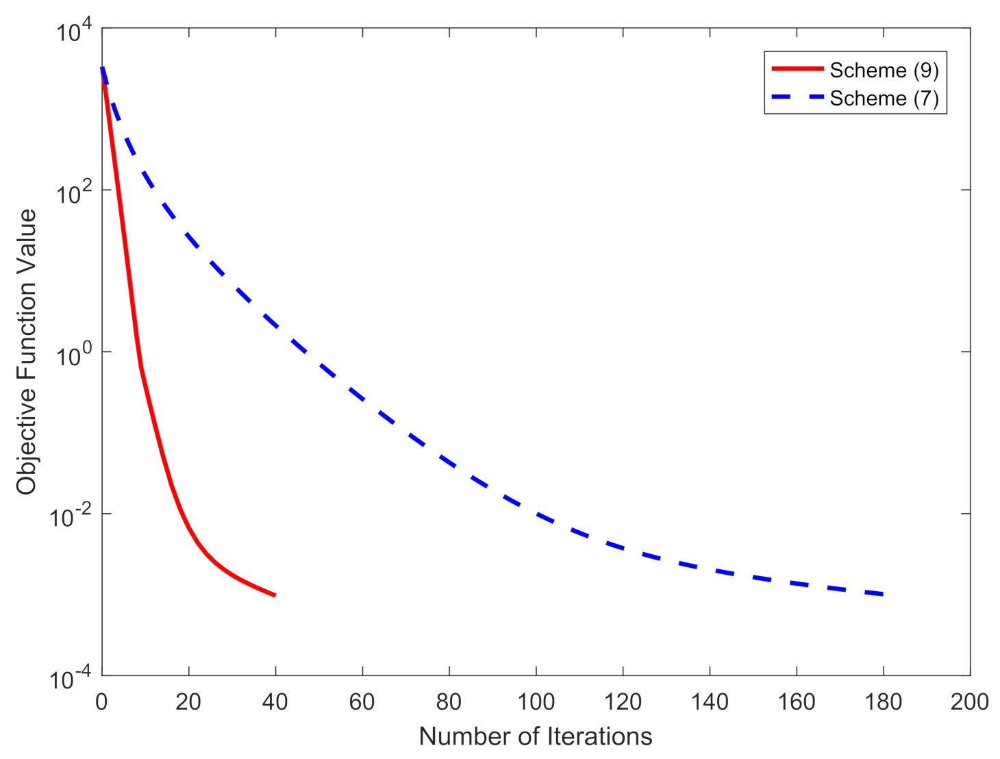
We give the parameters and initial values as follows: For (7) and (9), we choose ${\alpha }_n=\frac{1}{10n}$, ${\beta }_n=0.5$, ${\gamma }_n=0.5-\frac{1}{10n}$, ${\delta }_n=0.5$, $q_1={(1,1,1,1,1)}^{\mathrm{T}}$; for (7), we choose ${\tau }_n=\frac{1}{{\parallel A\parallel }^2}$; for (9), we choose ${ϵ}_n=\frac{1}{n^2}$, $\mu =1$, ${\rho }_n=3+\frac{1}{n+1}$, $q_0={(1,1,1,1,1)}^{\mathrm{T}}$. Denote $x^{*}$ by the solution of $Ax=b$. Then we have $x^{*}={(\frac{1}{16},\frac{1}{8},\frac{1}{4},\frac{1}{2},1)}^{\mathrm{T}}$. We can see that $x^{*}\in \mathrm{Fix}\left(S\right)$. We can see the numerical results of the main algorithms in Table 1 and Figure 1.

Table 1. Numerical results of scheme (9) as regards Example 1.

$\mathit{n}-1$	${\mathit{q}}_{\mathit{n}}^{\left(1\right)}$	${\mathit{q}}_{\mathit{n}}^{\left(2\right)}$	${\mathit{q}}_{\mathit{n}}^{\left(3\right)}$	${\mathit{q}}_{\mathit{n}}^{\left(4\right)}$	${\mathit{q}}_{\mathit{n}}^{\left(5\right)}$	${\mathit{E}}_{\mathit{n}}$
0	1.0000	1.0000	1.0000	1.0000	1.0000	1.5675 × 10${}^0$
10	0.2146	0.1868	0.2938	0.4159	0.8249	2.5806 × 10${}^{-1}$
50	0.0704	0.1281	0.2543	0.4935	0.9827	2.0782 × 10${}^{-2}$
100	0.0658	0.1263	0.2519	0.4971	0.9921	9.3812 × 10${}^{-3}$
500	0.0632	0.1253	0.2504	0.4994	0.9984	1.8944 × 10${}^{-3}$
1000	0.0628	0.1251	0.2502	0.4997	0.9992	9.4829 × 10${}^{-4}$
5000	0.0626	0.1250	0.2500	0.4999	0.9998	1.8983 × 10${}^{-4}$
10000	0.0625	0.1250	0.2500	0.5000	0.9999	9.4925 × 10${}^{-5}$

Figure 1. Comparison of scheme (9) and scheme (7) in Example 1.

From Table 1, we can see that with the addition of iterative steps, $\left\{q_n\right\}$ is closer to the exact solution $x^{*}$. We can also see that these errors are closer to zero. Hence, we can conclude that our algorithm is reliable. From Figure 1, we can see that our method has fewer iterations than (7), therefore our method has more advantages.

Example 2.

Seeking the solution to the following problem:

$$min\left\{\frac{1}{2}{\parallel Ax-b\parallel }_2^2:x\in {\mathbb{R}}^s,{\parallel x\parallel }_1\le \tau \right\},$$

where $A:{\mathbb{R}}^s\to {\mathbb{R}}^m$, $m<s$ is the bounded linear operator, $b\in {\mathbb{R}}^m$ and $\tau >0$. A is a sparse matrix, and A is generated by a standard normal distribution. The uniform distribution on the interval (-2,2) generates a real sparse signal $x^{*}$. The position of random p is not equal to zero, and the rest remains at zero. We can then obtain the sample data $b=A{x}^{*}$.

The key is to seek the sparse solution of the linear system so that we can use method (9) to solve the problem.

We define $C=\{x:\parallel x{\parallel }_1\le \tau \}$, $Q=\left\{b\right\}$. Because the projection on C has no closed formal solution, we consider the subgradient projection to solve it. Assume that the convex function $c\left(x\right)$ and the level set $C_n$ are defined by the following equation:

$$c\left(x\right)={\parallel x\parallel }_1-\tau ,C_n=\{x:c(q_n+⟨{\varsigma }_n,x-q_n⟩)\le 0\},$$

then ${\varsigma }_n\in \partial c\left(q_n\right)$. Next, we can calculate the orthogonal projection on $C_n$ according to the following formula:

$$P_{C_n}\left(x\right)=\left\{\begin{array}{cc}x,\hfill & \mathrm{if}c\left(q_n\right)+⟨{\varsigma }_n,x-q_n⟩\le 0,\hfill \\ x-\frac{c\left(q_n\right)+⟨{\varsigma }_n,x-x_n⟩}{\parallel {\varsigma }_n{\parallel }^2},\hfill & \mathrm{otherwise}.\hfill \end{array}\right.$$

Note that the subdifferential $\partial c$ on $q_n$ is the following:

$$\partial c\left(q_n\right)=\left\{\begin{array}{cc}1,\hfill & if{q}_n>0,\hfill \\ \left[-1,1\right],\hfill & if{q}_n=0,\hfill \\ -1,\hfill & if{q}_n<0.\hfill \end{array}\right.$$

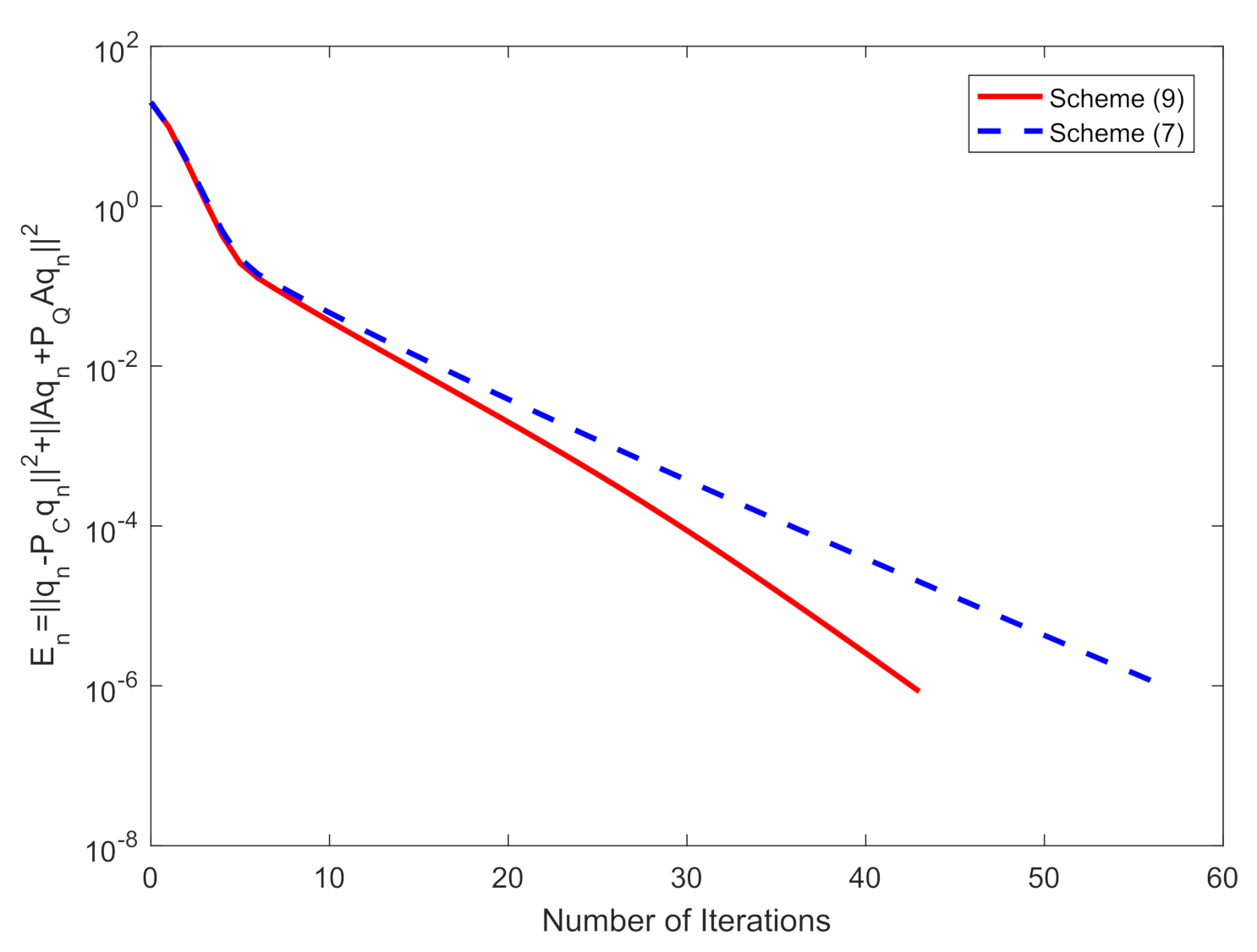
Let $S=I$, $g=0.4I$. Take $\frac{1}{2}{\parallel A{q}_n-b\parallel }_2^2\le {10}^{-3}$ as the stopping criterion. We give the parameters and initial values as follows: For (7) and (9), we choose ${\alpha }_n=\frac{1}{10n}$, ${\beta }_n=0.5$, ${\gamma }_n=0.5-\frac{1}{10n}$, ${\delta }_n=0.2$, $q_1={(1,1,\cdots ,1)}^{\mathrm{T}}$; for (7), we choose ${\tau }_n=\frac{1}{{\parallel A\parallel }^2}$; for (9), we choose ${ϵ}_n=\frac{1}{n^2}$, $\mu =1$, ${\rho }_n=2$, $q_0={(1,1,\cdots ,1)}^{\mathrm{T}}$. We can see the numerical results of the main algorithms in Table 2. Figure 2 shows that when $(m,s,p)=(240,1024,30)$, we can obtain the relationship between the target function and the iterations.

Table 2. Numerical results of scheme (9) and scheme (7) as regards Example 2.

m	s	p	Scheme (9)		Scheme (7)
			Iter.	Time (s)	Iter.	Time (s)
240	1024	30	40	0.0584	181	1.7113
480	2048	60	98	0.0933	337	13.8633
720	3072	90	142	0.1578	455	50.5543
960	4096	120	117	0.2073	544	138.2107
1200	5120	150	246	0.3534	795	706.2521
1440	6144	180	291	0.5483	883	1029.8199

Figure 2. Comparison of scheme (9) and scheme (7) in Example 2, with $(m,s,p)=(240,1024,30)$.

From Table 2 and Figure 2, we can see that our iterative method has advantages in both reaction time and the number of iterations.

Example 3.

Let $H_1=H_2=L_2[0,1]$, with the inner product given by the following:

$$⟨f,g⟩={\int }_0^{1}f\left(t\right)g\left(t\right)dt.$$

Let $C=\{x\in L_2[0,1]:\parallel x\parallel \le 1\}$, $Q=\left\{x\in L_2[0,1]:⟨x,\frac{t}{2}⟩=0\right\}$ and $\left(Ax\right)\left(t\right)=\frac{x\left(t\right)}{2}$. Let $S=I$, $g=0.5I$. Take $\parallel q_n-P_C{q}_n{\parallel }^2+{\parallel A{q}_n-P_{Q}A{q}_n\parallel }^2\le {10}^{-6}$ as the stopping criterion.

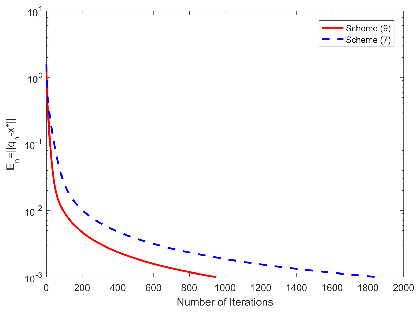
We then give the parameters and initial values as follows: For (7) and (9), we choose ${\alpha }_n=0.5n^{-0.7}$, ${\beta }_n=0.5$, ${\gamma }_n=0.5-0.5n^{-0.7}$, ${\delta }_n=0.5$; For (7), we choose ${\tau }_n=\frac{1}{{2\parallel A\parallel }^2}$; For (9), we choose ${ϵ}_n=0.25n^{-1.4}$, $\mu =0.5$, ${\rho }_n=1$, $q_0=q_1$. The numerical results for each choice of $q_1$ are shown in Table 3. Figure 3 shows that the error plotting for $q_1=4t^2+t+3$.

Table 3. Numerical results of scheme (9) and scheme (7) as regards Example 3.

${\mathit{q}}_1$	Scheme (9)		Scheme (7)
	Iter.	Time (s)	Iter.	Time (s)
$4t^2+t+3$	43	0.0413	57	0.0261
$e^t+2t$	37	0.0406	55	0.0249
$2^t/16$	10	0.0338	25	0.0146
$t^3+sint$	21	0.0363	46	0.0208

Figure 3. Comparison of scheme (9) and scheme (7) in Example 3, with $q_1=4t^2+t+3$.

5. Conclusions

In this paper, we proposed a new method to solve the SFP and the fixed-point problem involving quasi-nonexpansive mappings. Compared with the work of (7), the conditions were relaxed, and the nonexpansive mapping was extended to quasi-nonexpansive mapping. The inertia was also added to accelerate the convergence rate further. In addition, the selection of step size no longer depended on the operator norm.

By solving some examples, we have illustrated the effectiveness and practicability of the method. We compared all numerical implementations of this method with (7). As shown in Figure 1 and Figure 2, we can find that (9) is superior. For these reasons, we can see that (9) is more effective than (7).

References

- Censor, Y.; Elfving, T. A multiprojection algorithm using Bregman projections in a product space. Numer. Algor. 1994, 8, 221–239. [Google Scholar] [CrossRef]
- Byrne, C. Iterative oblique projection onto convex set and the split feasibility problem. Inverse Probl. 2002, 18, 441–453. [Google Scholar] [CrossRef]
- Xu, H.K. Iterative methods for the split feasibility problem in infinite-dimensional Hilbert spaces. Inverse Probl. 2010, 26, 105018. [Google Scholar] [CrossRef]
- López, G.; Martín-Márquez, V.; Wang, F.; Xu, H.K. Solving the split feasibility problem without prior knowledge of matrix norms. Inverse Probl. 2012, 28, 085004. [Google Scholar] [CrossRef]
- Qin, X.; Wang, L. A fixed point method for solving a split feasibility problem in Hilbert spaces. Rev. R. Acad. Cienc. Exactas Fís. Nat. Ser. A Mat. RACSAM 2019, 13, 215–325. [Google Scholar] [CrossRef]
- Kraikaew, R.; Saejung, S. A simple look at the method for solving split feasibility problems in Hilbert spaces. Rev. R. Acad. Cienc. Exactas Fís. Nat. Ser. A Mat. RACSAM 2020, 114, 117. [Google Scholar] [CrossRef]
- Kesornprom, S.; Pholasa, N.; Cholamjiak, P. On the convergence analysis of the gradient-CQ algorithms for the split feasibility problem. Numer. Alogr. 2020, 84, 997–1017. [Google Scholar] [CrossRef]
- Dong, Q.L.; He, S.; Rassias, T.M. General splitting methods with linearization for the split feasibility problem. J. Global Optim. 2021, 79, 813–836. [Google Scholar] [CrossRef]
- Shehu, Y.; Dong, Q.L.; Liu, L.L. Global and linear convergence of alternated inertial methods for split feasibility problems. Rev. R. Acad. Cienc. Exactas Fís. Nat. Ser. A Mat. RACSAM 2021, 115, 53. [Google Scholar] [CrossRef]
- Yang, J.; Liu, H. Strong convergence result for solving monotone variational inequalities in Hilbert space. Numer. Algor. 2019, 80, 741–752. [Google Scholar] [CrossRef]
- Kraikaew, R.; Saejung, S. Strong convergence of the Halpern subgradient extragradient method for solving variational inequalities in Hilbert spaces. J. Optim. Theory Appl. 2014, 163, 399–412. [Google Scholar] [CrossRef]
- Xu, H.K. Averaged mappings and the gradient-projection algorithm. J. Optim. Theory Appl. 2011, 150, 360–378. [Google Scholar] [CrossRef]
- Wang, Y.; Yuan, M.; Jiang, B. Multi-step inertial hybrid and shrinking Tseng’s algorithm with Meir-Keeler contractions for variational inclusion problems. Mathematics 2021, 9, 1548. [Google Scholar] [CrossRef]
- Jiang, B.; Wang, Y.; Yao, J.C. Multi-step inertial regularized methods for hierarchical variational inequality problems involving generalized Lipschitzian mappings. Mathematics 2021, 9, 2103. [Google Scholar] [CrossRef]
- He, S.; Yang, C. Solving the variational inequality problem defined on intersection of finite level sets. Abstr. Appl. Anal. 2013, 2013, 942315. [Google Scholar] [CrossRef]
- Byrne, C. A unified treatment of some iterative algorithms in signal processing and image reconstruction. Inverse Probl. 2004, 20, 103–120. [Google Scholar] [CrossRef] [Green Version]
- Tian, M.; Xu, G. Inertial modified Tsneg’s extragradient algorithms for solving monotone variational inequalities and fixed point problems. J. Nonlinear Funct. Anal. 2020, 2020, 35. [Google Scholar]
- Wang, Y.H.; Xia, Y.H. Strong convergence for asymptotically pseudocontractions with the demiclosedness principle in Banach spaces. Fixed Point Theory Appl. 2012, 2012, 45. [Google Scholar] [CrossRef] [Green Version]
Publisher’s Note: MDPI stays neutral with regard to jurisdictional claims in published maps and institutional affiliations. |
© 2022 by the authors. Licensee MDPI, Basel, Switzerland. This article is an open access article distributed under the terms and conditions of the Creative Commons Attribution (CC BY) license (https://creativecommons.org/licenses/by/4.0/).