Spatiotemporal Adaptive Fusion Graph Network for Short-Term Traffic Flow Forecasting

Abstract

Traffic flow forecasting is challenging for us to analyze intricate spatial–temporal dependencies and obtain incomplete information of spatial–temporal connection. Existing frameworks mostly construct spatial and temporal modeling based on a fixed graph structure and given time series. However, a fixed adjacency matrix is limited to learn effective spatial–temporal correlations of the network because it represents incomplete information for missing genuine relation. To solve the difficulty, we design a novel spatial–temporal adaptive fusion graph network (STFAGN) for traffic prediction. First, our model combines fusion convolution layers with a novel adaptive dependency matrix by end-to-end training to capture the hidden spatial-temporal dependency on the data to complete incomplete information. Second, STFAGN could, in parallel, acquire hidden spatial–temporal dependencies by a fusion operation and temporal trend by fast-DTW. Meanwhile, we use ReZero connection as a simple change of deep residual networks to facilitate deep signal propagation and faster converge. Lastly, we conduct comparative experiments on two public traffic network datasets, whose results demonstrate the superiority of our algorithm compared to state-of-the-art baseline types. Ablation experiments also prove the rationality of the framework of STFAGN.

1. Introduction

The number of vehicles increases on roads with the fast development of urbanization and the improvement of people’s living standards. Ubiquitous deployment of intelligent traffic systems (ITS) is one of the effective ways to alleviate urban traffic congestion [1]. Intelligent traffic systems are fast growing with the development of sensor technology, which enable dynamic traffic data collection to predict the future traffic flow of a road network [2]. Accurate traffic flow forecasting is promising in prompting urban traffic transportation [3,4].

Traffic flow forecasting is a challenging task. The methods in traffic forecasting can be divided into two categories: knowledge-driven methods and data-driven methods. In the early stage, queuing theory and simulating behaviors are applied in knowledge-driven methods [5]. With the rapid growing of traffic data collection and storage technologies, data-driven methods become increasingly popular. The statistical and machine learning method belong to the data-driven method, such as auto-regressive integrated moving average (ARIMA) [6], vector auto-regression (VAR) [7], support vector regression (SVR) [8,9] and Kalman filtering [10,11]. However, most of these methods are limited by the stationarity assumption of time series [12]. Thus, the performance is limited for capturing feature representation, especially for the high nonlinear dynamic traffic flow.

Deep learning approaches are not limited by the stationarity assumption, having better performance on time series prediction, as recurrent neural networks (RNNs) [13], long short-term memory (LSTM) [14] networks, and gated recurrent unit (GRU) [15] are widely applied in capturing the temporal correlations from a huge number of sequence information. However, these methods treat the traffic flow from different roads as independent patterns and fail to take into account the spatial information from traffic data. Different roadways may share the same pattern at the same time due to their similar road structure, or the traffic condition of the roadway in the previous time will have an impact on the other roadway the next time. In a graph neural network, the graph convolutional network has been proposed to exploit local spatial features through the Laplacian matrix [16]. For example, the dynamic graph convolutional recurrent network (DGCRN) [17], diffusion convolutional recurrent neural network (DCRNN) [18] and spatio-temporal graph convolutional network (STGCN) [19] capture correlations in spatial and temporal features by combining the recurrent neural networks and graph neural networks.

Although RNN- and GCN-based models have achieved successful performance in the final prediction, they still have shortcomings. First, most methods use the pre-defined adjacency or static graph structure to capture spatial and temporal dependency, and fail to dynamically exploit spatial–temporal dependency among nodes [20,21]. Although two nodes are connected in pre-defined graph, they have distinctive traffic features. For example, one end of a road is a commercial area, which is usually busy, and the other end is an industrial area, which is usually smooth [22]. On the other hand, some circumstances, such as office areas, school areas, or marketing areas, share similar traffic conditions although there is no connection between them in pre-defined adjacency during commuting time. With the static graph, it is hard to model the dynamic connection property between each traffic node. Second, exiting methods lack temporal graph construction [23]. When applying a given spatial adjacency matrix for graph convolution, they ignore the temporal similarity between nodes. Self-adaptive matrices are proposed to adjust the fixed spatial adjacency matrix [22,24]. However, the learned adjacency matrix does not effectively model the temporal graph to extract complicated spatial–temporal dependencies.

In this paper, we present a deep learning based method named the spatial–temporal adaptive fusion graph network (STAFGN) to address these two shortcomings. To achieve this, we propose a novel adaptive dependency matrix in the fusion convolution layer to preserve the hidden spatial–temporal dependency in traffic data. Then, we fuse spatial and temporal graphs in different time periods to capture in parallel the hidden spatial–temporal dependencies. Furthermore, we formulate the temporal adjacency matrix to measure temporal distances by fast-DTW [21] to extract the global temporal dependency more effectively. This paper first introduces the related work of others in traffic flow, and then proposes STAFGN. Finally, we conduct comparison and ablation experiments to demonstrate the effectiveness of the model. The main contributions of this work are as follows.

• We design the temporal adjacency matrix to effectively capture temporal distances of the traffic flow, and the adaptive matrix to exploit hidden spatial dependency in the static graph structure.
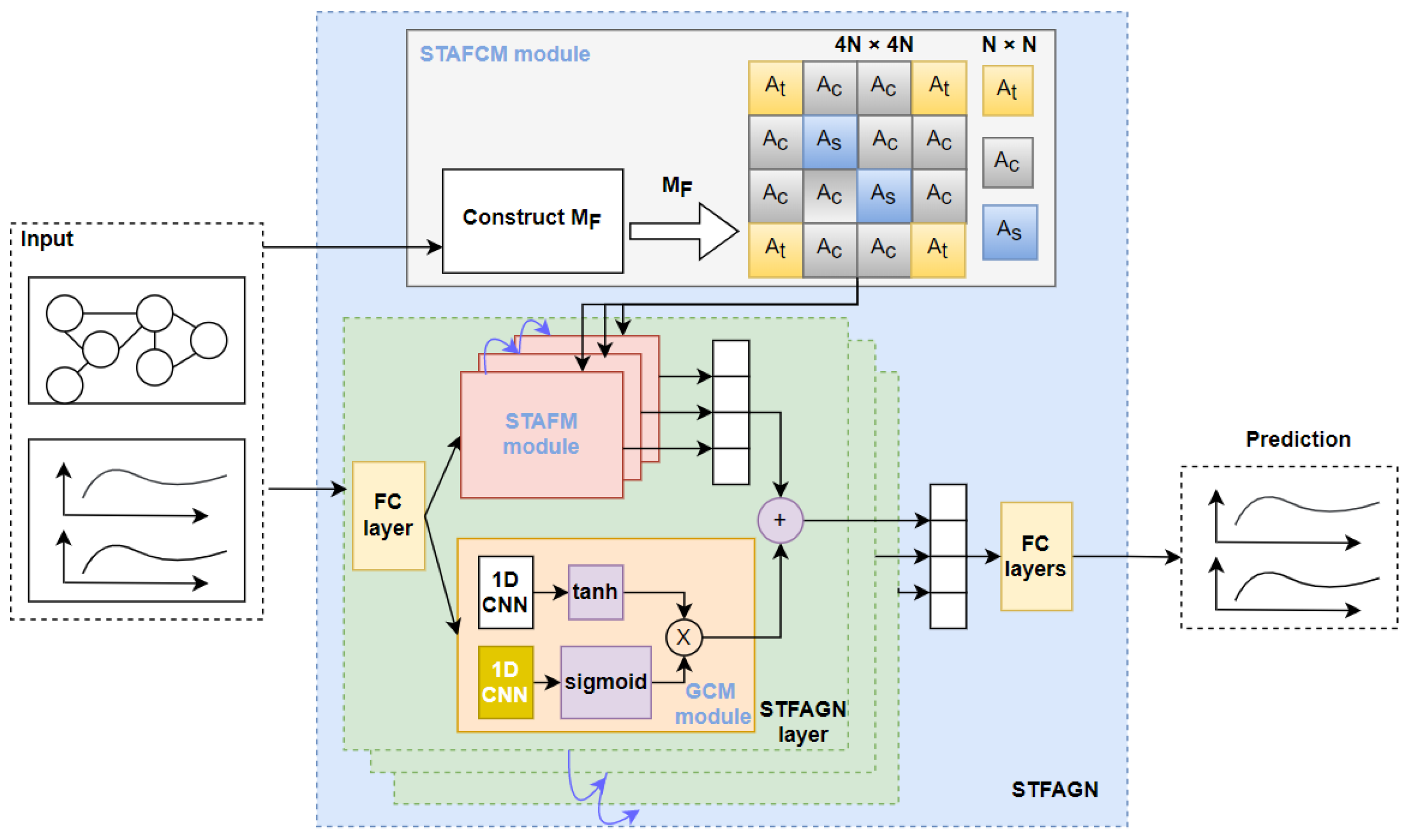
• We propose the spatial–temporal adaptive fusion graph network (STAFGN) to exploit spatial–temporal dependencies simultaneously by fusing the spatial and temporal graphs into a large adjacency matrix.
• We evaluate our model on two real-word traffic datasets with extensive experiments. The case study demonstrates that the STAFGN outperforms the state-of-the art methods.

2. Related Works

2.1. Traffic Flow Forecasting

A road network can be represented as $G=(V,E,A)$, where V is the set of nodes $\left|V\right|=N^2$, and E is the set of edges in the network. The spatial adjacency matrix is represented as $A\in {\mathbb{R}}^{N\times N}$. If there is an edge between $v_i$ and $v_j$, $A_{ij}$ is 1 and otherwise 0. At each time step t, $X_t\in {\mathbb{R}}^{N\times D}$ denotes the traffic status, e.g., road network occupancy, traffic speed, and capacity, in the road network. Traffic flow forecasting is to learn function f to map the historical traffic flow $X_{(t-P+1):t}$ to that of the future $X_{(t+1):(t+Q)}$.

$$\left[X_{(t-P+1):t},G\right]\stackrel{f}{\to }{\hat{X}}_{(t+1):(t+Q)},$$

(1)

where $X_{(t-P+1):t}=(X_{t-P+1},X_{t-P+2},\dots ,X_t)\in {\mathbb{R}}^{P\times N\times D}$ and ${\hat{X}}_{(t+1):(t+Q)}=({\hat{X}}_{t+1},{\hat{X}}_{t+2},\dots ,{\hat{X}}_{t+Q})\in {\mathbb{R}}^{P\times N\times D}$.

Traffic flow forecasting focuses on spatial–temporal forecasting [25]. The methods in spatial–temporal forecasting are classified in two categories, RNN-based [17,26] and CNN-based [21,24]. Now, many research studies employ the graph convolutional network in spatial–temporal forecasting. It has prompted the development of spatial–temporal forecasting, exploiting the spatial–temporal dependencies more effectively. The dynamic graph convolutional recurrent network (DGCRN) [17] model, a hyper-network to generate the dynamic adjacency matrix, was integrated with the static graph in GCN model to train. Graph WaveNet [24] uses the self-adaptive adjacency to preserve the implicit spatial dependencies and stacked dilated casual convolutions to exploit the temporal dependencies. Spatial–temporal fusion graph neural networks (STFGNN) [21] construct several graphs, which are integrated as a spatial–temporal fusion graph to explore the spatial–temporal relationship simultaneously.

2.2. Graph Convolution Networks

Graph convolution networks can be viewed as the process of graph-based presentation learning, aiming to utilize deep learning in structured data. It is widely applied in node classification [27], graph classification [28], and link prediction [29]. Spectral domain based and spatial domain based are the two main approaches in GCN. The spectral-domain-based method uses graph Fourier transform on the graph signal to deconstruct the graph signal in the spatial domain. The graph spectral filtering by decomposition of the Laplace matrix to exploit irregular graph data is as follows:

$$\gamma \star g\left(x\right)=\gamma \left(L\right)x=U\gamma (\Lambda )U^{T}x,$$

(2)

where $U\in {\mathbb{R}}^{n\times n}$ is eigenvectors of the Laplacian matrix $L=I_n-D^{-\frac{1}{2}}=U\lambda U\in {\mathbb{R}}^{n\times n}$, ($I_n$ is the identify matrix, $D\in {\mathbb{R}}^{n\times n}$ is the diagonal degree matrix with $D_{ii}={\sum }_j{W}_{ij}$), $\Lambda \in {\mathbb{R}}^{n\times n}$ is the diagonal matrix of eigenvectors of L, and $\gamma (\Lambda )$ is the spectral filter, which is also a diagonal matrix.

Different from the spectral domain, the spatial-based method aggregates features from the spatial neighbor to learn a high-dimension representation. GraphSAGE [30] focuses on node central mini-batch training by the aggregation of its neighbors, enabling distributed training on large-scale data. GAT [31] uses the attention mechanism to aggregate neighbor nodes, realizing adaptive allocation to different neighbor weights.

2.3. Fast-DTW

Fast dynamic time warping (fast-DTW) is the modified algorithm based on dynamic time warping (DTW) [32]. DTW is a classical algorithm to measure the time series similarity, as well as the Euclidean distance [33]. However, in most situations, two times series have very similar shapes as a whole; these shapes are not aligned on the x axis. So, before comparing time series similarity, one of the time series needs to be warped under the timeline for better alignment. DTW is an effective way to achieve this warping distortion [34]. It calculates the similarity between two time series by extending and shortening the time series.

Given two time series $X=(x_1,x_2,\cdots ,x_n)$ and $Y=(y_1,y_2,\cdots ,y_m)$, the state transition $d{p}_{n\times m}$ can be generated as follows:

$$dp(i,j)=min\left(dp\right(i-1,j-1),dp(i-1,j),dp(i,j-1\left)\right)+d(i,j),$$

(3)

where $d(i,j)$ is the distance between $x_i$ and $y_j$. After several iterations, $dp{(n,m)}^{\frac{1}{2}}$ is the similarity between time series X and Y.

While calculating state transition $d{p}_{n\times m}$, the warping path $\Phi$ can be generated from it. The warping path $\Phi$ is denoted as follows:

$$\varphi =(w_1,w_2,\cdots ,w_{\lambda }),max(n,m)\le \lambda \le n+m,$$

(4)

where $w_{\lambda }$ means the matchup between $x_i$ and $y_j$.

However, since the real traffic time series is large, utilizing DTW to the general series similarity based on real traffic data is a challenging task. The computational complexity is up to $O\left(n^2\right)$. To address this problem, STFGCN [21] limits the search length T to improve the DTW algorithm, which is named fast-DTW. The searching range is restricted as follows:

$$w_k=(i,j),|i-j|\le T$$

(5)

In Equation (3), we can see that the computation complexity is declined from $O\left(n^2\right)$ to $O\left(Tn\right)$, making it possible to calculate the large and long traffic data.

2.4. ReZero

Trainability is related to dynamic isometry [35]. ReZero (residual with zero initialization) is a way to ensure initial dynamical isometry in deep networks [36]. It add learnable parameters to the architecture of deep residual network in order to dynamically promote well-behaved gradients and arbitrarily deep signal propagation. A skip connection and residual weights ${\alpha }_i$ are used to realize the non-trivial transformation of a layer $F\left(x\right)$. The propagation is shown below:

$$x_{i+1}=x_i+{\alpha }_{i}F\left(x_i\right)$$

(6)

3. Methodology

As shown in Figure 1, our spatial–temporal adaptive fusion graph convolution network consists of three modules, including the spatial–temporal adaptive fusion construction module (STAFCM), the spatial–temporal adaptive fusion graph neural module (STAFM) and the gated convolution module (GCM). First, the STAFCM constructs the spatial–temporal fusion adjacency matrix $M_F$ to integrate spatial–temporal information. The proposed $M_F$ contains the temporal adjacency matrix $A_t$ computed by fast-DTW [21], the spatial adjacency matrix $A_s$ and the temporal connectivity graph $A_c$ to represent given spatial–temporal connections in the traffic graph. The combination of $M_F$ is displayed in the STAFCM of Figure 1, with blue for $A_s$, orange for $A_t$, and gray for $A_c$. Second, the STAFM completes the incomplete fusion adjacency matrix $M_F$ in the fusion self-adaptive convolution layer for hidden spatial–temporal features in gated multiplication layers. Basically, the STAFM is composed of a fusion self-adaptive convolution layer and stacked gated multiplication layers with a max pooling layer. The fusion self-adaptive convolution layers learn the adjacency matrix from data through an end-to-end supervised training to construct the self-adaptive fusion adjacency matrix ${\tilde{M}}_F$. The gated multiplication layers aggregate the spatial–temporal dependencies by matrix multiplication from ${\tilde{M}}_F$. Third, the GCM extracts long-range spatial–temporal dependencies by a large dilation rate as a gating mechanism in recurrent neural networks. We stacked k STFAGN layers to capture hidden spatial–temporal dependencies.

3.1. Spatial–Temporal Adaptive Fusion Convolution Layer

In this paper, we design a spatial–temporal adaptive fusion convolution layer to extract long-term spatial–temporal dependencies in the GCM module. The layer also can establish the self-adaptive fusion adjacency matrix to supplement spatial–temporal connections in the STAFM module. In Figure 1, the STFAGN layer represents the spatial–temporal adaptive fusion convolution layer. The layer mainly consists of the GCM and STAFM module.

A fixed adjacency matrix is not relevant to prediction tasks, which may cause considerable biases. However, it is pricey to collecting complete and precise road information by sensors. To adjust the incomplete adjacency matrix, Wu et al. [24] introduced a self-adaptive adjacency matrix to construct and complement the adjacency matrix without prior knowledge by learnable node embedding. Given two introduced node embedding $M_i,M_j\in {\mathbb{R}}^{N\times D}$, the self-adaptive adjacency matrix is $\tilde{M}=\sigma (\phi (M_i{M}_j^T))$, where $\sigma (·)$. $\phi (·)$ respectively denotes the softmax and ReLU activation function. Supposing that a graph is directed, the diffusion direction is double, comprising forward and backward directions. They gave a definition to a forward transition matrix as $S_f=A/{\sum }_{i=0}^n{A}_{ij}$ and a backward transition matrix as $S_b=A^T/{\sum }_{i=0}^n{A}_{ij}^T$ [24]. They integrated the diffusion convolution layer with the self-adaptive adjacency matrix and defined the diffusion self-adaptive convolution layer as

$$Y=\sum _{k=0}^K{\tilde{M}}^{k}X{W}_{ka}+S_f^{k}X{W}_{kf}+S_f^{b}X{W}_{kb},$$

(7)

3.2. Spatial–Temporal Adaptive Fusion Construction Module

We present the STAFCM module to aggregate spatial–temporal dependencies in the spatial–temporal fusion adjacency matrix. As displayed in Figure 1, the spatial–temporal fusion adjacency matrix $M_F\in {\mathbb{R}}^{KN\times KN}$ consists of the temporal adjacency matrix $A_t\in {\mathbb{R}}^{N\times N}$ computed by fast-DTW [21], the spatial adjacency matrix $A_s\in {\mathbb{R}}^{N\times N}$ and the temporal connectivity graph matrix $A_c\in {\mathbb{R}}^{N\times N}$ [21]. Fast-DTW is applied to construct the temporal adjacency matrix $A_t$. We add the similarity of temporal trends into an adjacency matrix with fast-DTW from Equations (3) and (4). $A_c$ represents the connection of the same node belonging to the recent time step. In each node $l\in \left\{1,2,\dots ,N\right\}$, when $i=t\times N+l$ and $j=(t+1)\times N+l$, $M_{F,ij}=1$, where t is the current time step. Each node could integrate the spatial relevance from $A_s$, temporal pattern information from $A_t$ and its own approximate correlation of the proximal time step from $A_c$ by matrix multiplication with $M_F$. In this paper, K defaults to 4. Let $A_t$ denote the temporal adjacency matrix to obtain the temporal information of the time sequence. $A_s$ is given from the fixed dataset. Finally, as Figure 1 shows, the spatial–temporal fusion adjacency matrix $M_F$ is constructed.

The input of the STAFM module is formulated into $H^0=\left[X^{\left(t\right)},X^{(t+1)},\cdots ,X^{(t+K)}\right]\in {\mathbb{R}}^{K\times N\times D\times C},$ where $X^{\left(t\right)}$ is separated from all series $X=\left[X^{\left(t\right)},X^{(t+1)},\cdots ,X^{(t+T)}\right]\in {\mathbb{R}}^{T\times N\times D\times C}$. C denotes the number of channels in the STAFM module.

3.3. Gated Convolution Module

We design the GCM module to capture the long-term spatial–temporal information with a large dilation rate. Gating mechanisms in recurrent neural networks make a difference to extracting the long-term relevance of traffic flow with gated temporal convolutions [37]. Gated TCN with dilation factor k (e.g., 1, 2, and 4) can learn complicated temporal correlation [24]. However, because the GCM employs a larger dilation rate, the GCM module is distinct from TCN in Graph WaveNet [24] and STGCN [38] by extracting more long-range spatial–temporal dependencies. Given the whole input data $X\in {\mathbb{R}}^{T\times N\times d\times C}$, it takes the following form:

$$Z=\sigma ({\Phi }_1*X+b_1)\odot \varphi ({\Phi }_2*X+b_2),$$

(8)

where $\sigma (·)$ and $\varphi (·)$ are sigmoid and tanh functions. Importantly, ${\Phi }_1$ and ${\Phi }_2$ stand for two 1D convolution with dilation factors $=K-1$, which controls the skipping distance to enlarge the receptive field along the time axis [24].

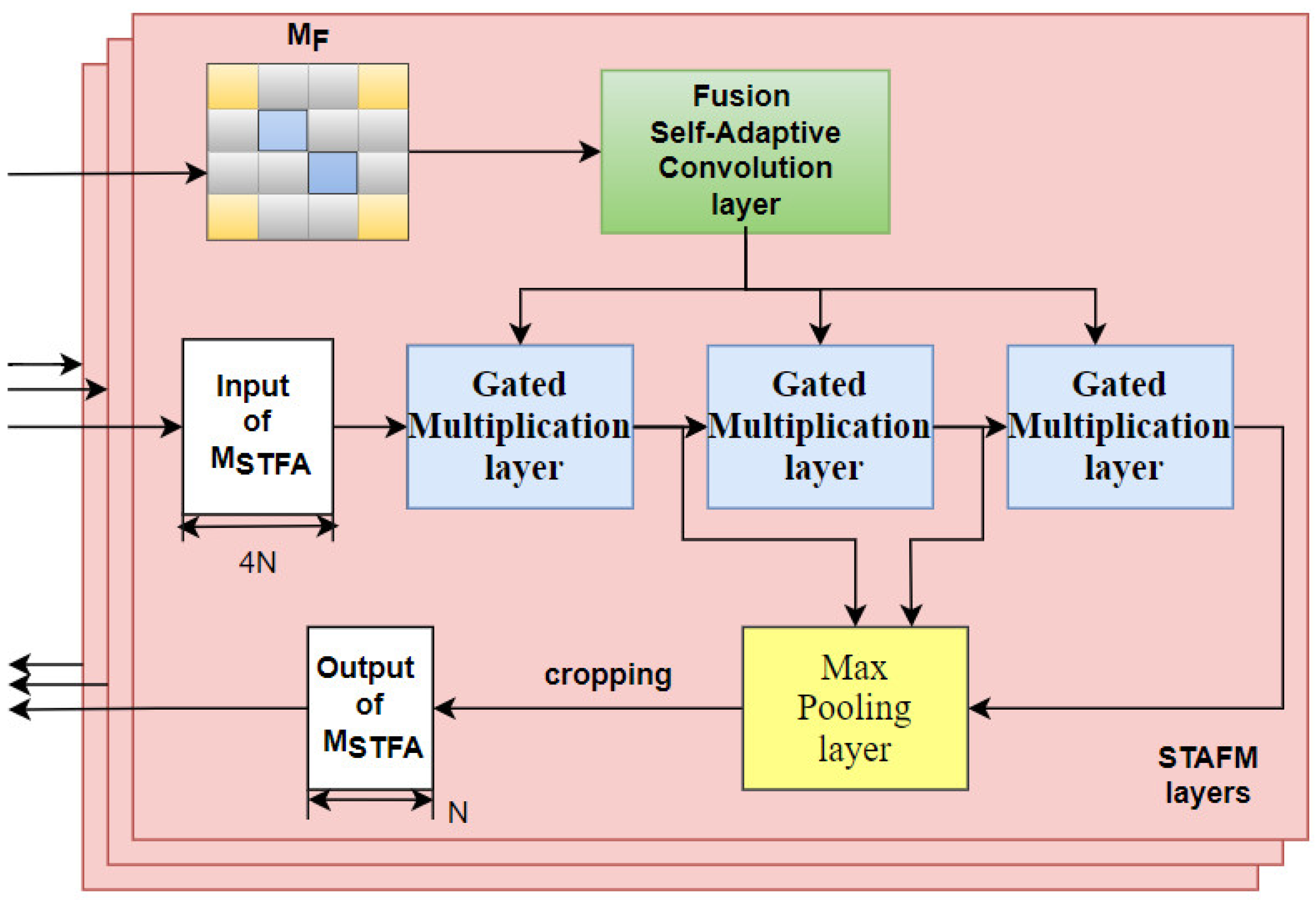
3.4. Spatial–Temporal Adaptive Fusion Graph Neural Module

Figure 2 displays the STAFM module serving as a deep convolution learnable model, capturing hidden spatial–temporal features to complement the incomplete spatial–temporal connection. The STAFM module is made up of the fusion self-adaptive convolution layer, and stacks the gated multiplication layers followed by the max pooling layer with ReZero connection. Li et al. [21] introduced the STFGN module in the STFGNN to capture complicated correlations by multiplying the STFGN modules independently in parallel. However, the STFGN module cannot adaptively complete an incomplete connection of the graph. Compared with STFGNN, the novel STAFM module constructs the fusion adjacency matrix of the spatial–temporal relationship to complete the incomplete spatial–temporal adjacency matrix.

Fusion Self-Adaptive Convolution layer: Based on the spatial–temporal fusion adjacency matrix and the diffusion self-adaptive convolution layer, we propose a fusion self-adaptive convolution layer (FSAC) to adaptively learn the self-adaptive fusion adjacency matrix ${\tilde{M}}_F\in {\mathbb{R}}^{KN\times KN}$ by an end-to-end learnable convolution layer. ${\tilde{M}}_F=softmax(ReLU(M_i{M}_j^T))$, where $M_i\in {\mathbb{R}}^{KN\times d}$ and $M_j\in {\mathbb{R}}^{KN\times d}$ are spatial–temporal fusion node embeddings of source and target nodes. $M_i$ and $M_j$ are learnable parameters. We adopt the ReLU activation function to alleviate the occurrence of overfitting. We define that $S_f=M_F/rowsum\left(M_F\right)$ and $S_b=M_F^T/rowsum\left(M_F^T\right)$. Lastly, the graph convolution layer with ${\tilde{M}}_F$ can be summed up as

$$Y=\sum _{k=0}^K{\tilde{M}}_F^{k}X{W}_F^k+S_b^{k}X{W}_f^k+S_f^{b}X{W}_b^k.$$

(9)

Gated Multiplication Layer: In a gated multiplication layer, we replace matrix multiplication for a spectral filter to integrate complicated spatial–temporal correlations in the graph multiplication layer. The gated multiplication layer can capture hidden spatial–temporal correlations by matrix multiplication. Therefore, in the STAFM layer, a graph multiplication layer aggregates matrix multiplication and GCM. In the graph multiplication layer, a gated linear unit can summarize global characteristics after nonlinear activation. We introduce the parameters of GLU with $W_1,W_2\in {\mathbb{R}}^{C\times C}$, ${\tilde{M}}_F\in {\mathbb{R}}^{KN\times C}$ and $b_1,b_2\in {\mathbb{R}}^{C\times C}$. Let $H^l,H^{l+1}\in {\mathbb{R}}^{KN\times C}$ denote the l-th hidden feature. Then, we formulate gated multiplication as

$$H^{l+1}=\sigma ({\tilde{M}}_F{H}^l{W}_1+b_1)\odot ({\tilde{M}}_F{H}^l{W}_2+b_2),$$

(10)

where ⊙ is the Hadamard product in GLU and $\sigma$ is the sigmoid. Different from residual connection [39,40], stacking layers with ReZero connections [36] are fast to obtain the complex spatial correlation of each layer. The next layer is the max pooling layer, which concatenates each hidden state $H^P\in maxPool\left([H^1,H^2,\dots ,H^L]\right)\in {\mathbb{R}}^{K\times N\times D\times C}$.

As illustrated in Figure 2, after the max pooling layer, $H^P$ is cut into the shape of ${\mathbb{R}}^{1\times N\times D\times C}$, which can represent complicated anisotropy [21]. There are $⌊\frac{T}{K-1}⌋-1$ layers stacked in the STAFM. As a consequence, the cropped connection of the intermediate time step is organized into $H^p=H^m\left[\left[\frac{K}{2}\right],\frac{K}{2}+1,:,:,:\right]\in R^{1\times N\times \times D\times C}$.

ReZero connection: We adopt ReZero connection in the STFAGN for faster training and convergence. Bachlechner et al. [40] demonstrated that ReZero has several benefits, including wide usability, deeper learning and faster convergence. Compared with residual connection, ReZero (residual with zero initialization) is a simple change in deep residual networks to facilitate dynamical isometry. It further enables the efficient training of extremely deep networks [36]. So, we substitute ReZero for residual connection [40]. Given $F\left[W_i\right]$, which includes the STAFM layer and STFAGN layer and so on, the signal now propagates according to

$$H_{i+1}=H_i+{\theta }_{i}F\left[W_i\right]\left(H_i\right),$$

(11)

where ${\theta }_i$ represents i-th learnable parameters, named residual weights [36].

Multiple STAFM layers operate the input signal in parallel to extract spatial–temporal dependencies by gated multiplication. The shape of output data ${\mathbb{R}}^{T\times N\times D\times C}$ is transformed into ${\mathbb{R}}^{(T-K+1)\times N\times D\times C}$. Let $\vartheta$ denote a hyperparameter to control the sensitivity of the squared error. We apply Huber loss as the loss function, whose specific calculation is shown as

$$L({\hat{X}}_G^{(t+1):(t+T)},\Theta )=\frac{{\sum }_{i=0}^T{\sum }_{j=0}^N{\sum }_{K=0}^{D}Er({\hat{X}}_G^{t+i},X_G^{t+i})}{T\times N\times D},$$

(12)

$$Er(\hat{Y},Y)=\left\{\begin{array}{ccc}\frac{1}{2}{(\hat{Y}-Y)}^2,& \left|\hat{Y}-Y\right|\le \vartheta & \\ \vartheta \left|\hat{Y}-Y\right|-\frac{1}{2}{\vartheta }^2,& \left|\hat{Y}-Y\right|>\vartheta \end{array}\right..$$

(13)

4. Experiments

4.1. Datasets and Baseline

Under the same hardware environment and the same datasets, we conduct comparative experiments to facilitate comparison with other advanced baselines. We testify the effectiveness of the STFAGN based on two traffic signal datasets consisting of METR-LA and PEMS-BAY [18]. METR-LA is constructed from records of highways in Los Angeles County, which tests traffic speeds with a sensor over a period of four months. PEMS-BAY comprises traffic speeds of the Bay area over a period of six months. For both datasets, sensors calculate traffic speed every 5 mins, so the adjacent time series differ by 5 mins. The sensors of METR-LA and PEMS-BAY add up to 207 and 325, respectively, with 1515 and 2369 edges. Before training data, there is a requirement to pre-process data, the same as in [18]. The adjacency matrix of both datasets is established on a distance-based graph with the threshold of a Gaussian kernel [17]. The datasets are separated in 70% for training, 20% for validation, and 10% for testing. For more details, see

Table 1. Statistical properties of METR-LA and PEMS-BAY.

Dataset	Timestep	Nodes	Edges
METR-LA	34,272	207	1515
PEMS-BAY	52,116	325	2691

.

We compare STFAGN with the following models.

• Graph WaveNet: Graph WaveNet, a spatial–temporal graph model with a stacked dilated 1D convolution component and self-adaptive adjacency layers [24].
• STFGNN: Spatial–temporal fusion graph neural networks, with a gated dilated CNN module and spatial–temporal fusion graph module in parallel [21].
• ARIMA: Autoregressive integrated moving average [6,41], with Kalman filter, widely used in time series analysis, which fits time series data to predict future points in the series.
• SVR: Support vector regression, using a support vector machine to regress traffic sequence, characterized by the use of kernels, sparse solution, VC control of the margin and the number of support vectors [8].

4.2. Experiments Results and Analysis

Our experiments are launched under an environment with Intel(R) Xeon(R) Gold 6139 CPU @ 2.30GHz. The edition of NVIDIA is NVIDIA-SMI 455.45.01, driver with version 455.45.01, and CUDA with Version 11.1. The temporal adjacency matrix At respectively generated from fast-DTW in Alg1. The sparsity of the temporal adjacency matrix $A_t$ is 0.01. The batch size is 32. The epoch of training is 100. The using learning rate of the Adam optimizer is $1.0\times {10}^{-3}$. In the STAFM, the number of gated multiplication layers is 3. The STFAGN includes 8 parallel STAFM layers with dilation rate 3 and 1 gated multiplication layer. The size of the filter in the model is $R^{3\times 3}$ with all elements filled with 64. Then, we let the dilation rate equal 3, because the size K of the spatial–temporal fusion adjacency matrix is 4 to aggregate information through the neighbor. For all experiments, we use 12 past time steps of traffic signal to predict 3, 6 and 12 time steps in the future.

Table 2. Effectiveness and consequence of STFAGN in comparison with Graph WaveNet, STFGNN, ARIMA and SVR. We trained every models five times to get five results and calculated the mean and standard deviation of the results.

Dataset	Models	15 min			30 min			60 min
		MAE	MAPE%	RMSE	MAE	MAPE%	RMSE	MAE	MAPE	RMSE
METR-LA	Graph WaveNet	2.98± 0.00	7.88± 0.00	5.91± 0.01	3.59± 0.00	10.17± 0.00	7.29± 0.01	4.45± 0.01	13.66± 0.00	8.97± 0.02
	STFGNN	2.99± 0.00	7.24± 0.05	6.72± 0.02	3.48± 0.00	8.69± 0.06	8.10± 0.03	4.27± 0.01	11.01± 0.08	10.00± 0.03
	STFAGN	2.94± 0.01	7.12± 0.06	6.62± 0.02	3.32± 0.06	8.22± 0.17	7.76± 0.16	3.96± 0.01	10.01± 0.08	9.46± 0.04
	ARIMA	3.99± 0.00	9.60± 0.00	8.21± 0.00	5.15± 0.00	12.70± 0.00	10.45± 0.00	6.90± 0.00	17.40± 0.00	13.23± 0.00
	SVR	3.99± 0.00	9.30± 0.00	8.45± 0.00	5.05± 0.00	12.10± 0.00	10.87± 0.00	6.72± 0.00	16.70± 0.00	13.76± 0.00
PEMS-BAY	GraptWaveNet	1.39± 0.00	2.90± 0.00	3.01± 0.00	1.84± 0.00	4.16± 0.13	4.22± 0.01	2.37± 0.01	5.85± 0.00	5.45± 0.01
	STFGNN	1.20± 0.01	2.47± 0.03	2.47± 0.04	1.47± 0.01	3.18± 0.05	3.27± 0.04	1.81± 0.00	4.17± 0.05	4.23± 0.04
	STFAGN	1.17± 0.00	2.43± 0.02	2.43± 0.02	1.41± 0.00	3.06± 0.02	3.13± 0.03	1.69± 0.00	3.85± 0.02	3.88± 0.03
	ARIMA	1.62± 0.00	3.50± 0.00	3.30± 0.00	2.33± 0.00	5.40± 0.00	4.76± 0.00	3.38± 0.00	8.30± 0.00	6.50± 0.00
	SVR	1.85± 0.00	3.80± 0.00	3.59± 0.00	2.48± 0.00	5.50± 0.00	5.18± 0.00	3.28± 0.00	8.00± 0.00	7.08± 0.00

indicates a comparison of the prediction validity of each model. The experiment is conducted to input and train the data of the past 60 min to predict the next 15, 30, and 60 min of traffic speed in the METR-LA and PEMS-BAY datasets. On the mean result of 60 min horizons in METR-LA, STFAGN is optimized by 3.56% more than Graph WaveNet, 1.00% more than STFGNN, 7.30% more than ARIMA and 6.60% more than SVR. On the mean result of PEMS-BAY in three horizons, STFAGN is probably increased by 0.1% to 2.5% compared to other baselines.

So, STFAGN surpasses data-driven approaches, such as ARIMA and SVR. Moveover, STFAGN outperforms the previous convolution-based models, including Graph WaveNet and STFGNN.

Traffic flow is nonlinear data with complex spatiotemporal correlation. ARIMA only captures linear relationships. SVR fails to adopt the spatial correlation of the traffic network. So, ARIMA and SVR perform poorly in traffic prediction. Graph WaveNet is conducted with poor performance, because it cannot construct the adaptive fusion spatial–temporal adjacency matrix with incomplete spatial–temporal relevance. Compared with STFGNN, the second best framework, the effectiveness of STFAGN is slightly better than it on 15 min and 30 min horizons, but significantly exceeds STFGNN on 60 min horizons. We consider that there are two reasons to explain the effectiveness of STFAGN. First, our model can be more adaptive to adjust the spatial–temporal adjacency matrix by constructing the spatial–temporal adaptive fusion layer. Second, STFAGN is more effective in extracting long-term temporal correlation by integrating the STAFM module with a gated CNN module.

In general, the average result of the presented STFAGN model is superior compared to the baselines in performance of extracting spatial–temporal relevance. From the standard deviation, the training results are also relatively stable.

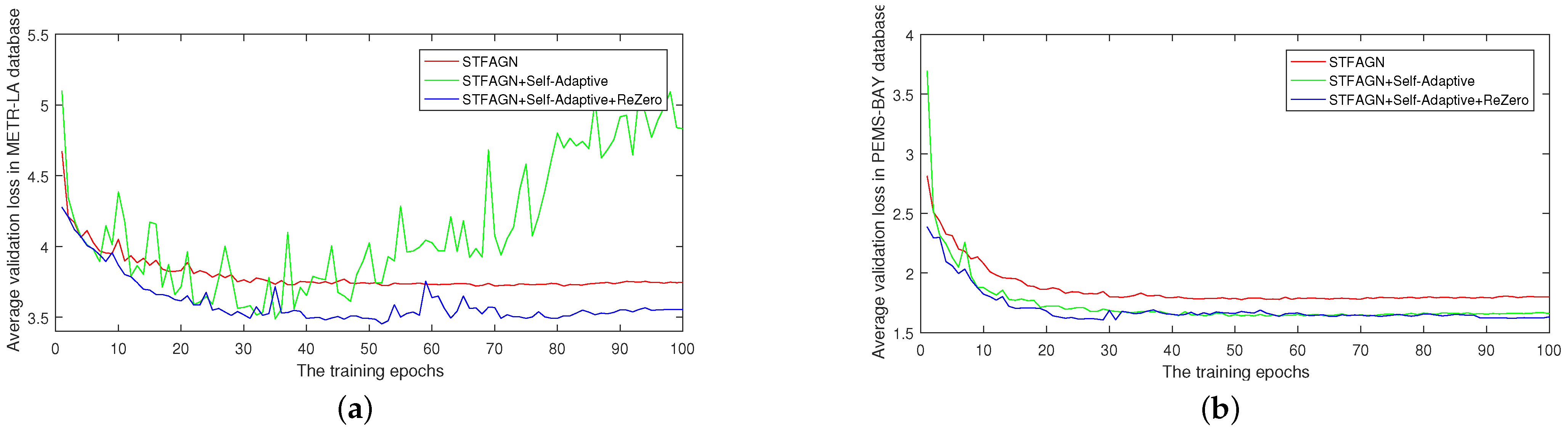
4.3. Ablation Experiments

To verify the significance of different components in STFAGN, we conduct ablation experiments on METR-LA and PEMS-BAY. “Model Elements” denote different configurations.

• $[M,no]$: STFAGN is not configured with adaptive matrix $\tilde{M}$ and ReZero connection.
• $[\tilde{M},no]$: STFAGN is configured with adaptive matrix $\tilde{M}$ without ReZero connection.
• $[\tilde{M},ReZero]$: STFAGN is configured with adaptive matrix $\tilde{M}$ with ReZero connection.

From the experiments in

Table 3. Ablation experiments on different configurations of modules in METR-LA and PEMS-BAY datasets. The default configuration we use in STFAGN is $\left[\tilde{M},ReZero\right]$. We retrained each model five times to get five results then calculated the mean and standard deviation of the results.

Dataset	Models	15 min			30 min			60 min
	Elements	MAE	MAPE%	RMSE	MAE	MAPE%	RMSE	MAE	MAPE%	RMSE
METR-LA	[M,no]	2.99± 0.00	7.24± 0.05	6.72± 0.02	3.48± 0.00	8.69± 0.06	8.10± 0.03	4.27± 0.01	11.01± 0.08	10.00± 0.03
	[$\tilde{M}$,no]	2.97± 0.03	7.14± 0.09	6.67± 0.09	3.39± 0.03	8.29± 0.07	7.90± 0.06	4.01± 0.03	10.00± 0.08	9.53± 0.05
	[$\tilde{M}$,Rezero]	2.94± 0.01	7.12± 0.06	6.62± 0.02	3.32± 0.06	8.22± 0.17	7.76± 0.16	3.96± 0.01	10.01± 0.08	9.46± 0.04
PEMS-BAY	[M,no]	1.20± 0.01	2.47± 0.03	2.47± 0.04	1.47± 0.01	3.18± 0.05	3.27± 0.04	1.81± 0.00	4.17± 0.05	4.23± 0.04
	[$\tilde{M}$,no]	1.18± 0.00	2.44± 0.03	2.53± 0.26	1.41± 0.00	3.07± 0.03	3.17± 0.15	1.69± 0.01	3.88± 0.04	3.90± 0.08
	[$\tilde{M}$,Rezero]	1.18± 0.01	2.42± 0.02	2.45± 0.06	1.41 ±0.00	3.05 ±0.02	3.12± 0.04	1.68± 0.00	3.81± 0.02	3.89± 0.07

and Figure 3, we draw the following conclusions concerning the proposed ideas:

• For the ingredient of $\tilde{M}$, the fusion self-adaptive convolution layer is used to construct the adaptive fusion adjacency matrix, which can complete incomplete information of the adjacency matrix in the traffic network. Traffic networks based on distance do not mean that adjacent nodes have a traffic information association. The self-adaptive fusion adjacency matrix $\tilde{M}$ just makes up for this information and achieves a good effect of accelerating convergence.
• ReZero, a simple architectural modification, facilitates signal propagation in deep networks and helps the network maintain dynamical isometry. Applying ReZero to the STFAGN, significantly improved convergence speeds can be observed.
• STFAGN with the adaptive fusion adjacency matrix and ReZero connection not only adjusts spatiotemporal dependency, but trains efficiently. Therefore, the design of the component is reasonable.

5. Conclusions

In this paper, we propose an innovative spatial–temporal network to forecast traffic data. We design the spatial–temporal adaptive fusion graph network to capture hidden spatial–temporal heterogeneity effectively. First, learnable spatial–temporal fusion adjacency adaptively adjusts the spatiotemporal connections. Second, we integrate the STAFM module with a gated CNN module, which effectively broadens the receptive field in the time dimension. Lastly, we replace the ReZero connection with a residual connection to enable faster convergence. Ablation experiments show that the design of the fusion adjacency matrix and ReZero connection is reasonable and effective. Executive experiments and analysis reveal the advantages and weaknesses of previous models, which in turn demonstrate STFAGN to be of great effectiveness and superiority.

We found that it is still challenging to effectively extract the dynamics of traffic data in both temporal and spatial dimensions. The proposed spatial–temporal graph convolution network fails to capture many dynamic spatial relations hiding in the traffic data. In the future, we plan to further analyze the dynamic characteristics of traffic networks to capture the dynamic spatial–temporal correlation.

References

1. Wei, H.; Zheng, G.; Yao, H.; Li, Z. Intellilight: A reinforcement learning approach for intelligent traffic light control. In Proceedings of the 24th ACM SIGKDD International Conference on Knowledge Discovery & Data Mining, London, UK, 19–23 August 2018; pp. 2496–2505. [Google Scholar]
2. Cai, W.; Yang, J.; Yu, Y.; Song, Y.; Zhou, T.; Qin, J. PSO-ELM: A Hybrid Learning Model for Short-term Traffic Flow Forecasting. IEEE Access 2020, 8, 6505–6514. [Google Scholar] [CrossRef]
3. Cai, L.; Zhang, Z.; Yang, J.; Yu, Y.; Zhou, T.; Qin, J. A noise-immune Kalman filter for short-term traffic flow forecasting. Phys. A Stat. Mech. Its Appl. 2019, 536, 122601. [Google Scholar] [CrossRef]
4. Zheng, S.; Zhang, S.; Song, Y.; Lin, Z.; Wang, F.; Zhou, T. A Noise-eliminated Gradient Boosting Model for Short-term Traffic Flow Forecasting. In Proceedings of the 8th International Conference on Digital Home, Dalian, China, 19–20 September 2020. [Google Scholar]
5. Cascetta, E. Transportation Systems Engineering: Theory and Methods; Springer Science & Business Media: Cham, Switzerland, 2013; Volume 49. [Google Scholar]
6. Kumar, S.V.; Vanajakshi, L. Short-term traffic flow prediction using seasonal ARIMA model with limited input data. Eur. Transp. Res. Rev. 2015, 7, 21. [Google Scholar] [CrossRef] [Green Version]
7. Lippi, M.; Bertini, M.; Frasconi, P. Short-term traffic flow forecasting: An experimental comparison of time-series analysis and supervised learning. IEEE Trans. Intell. Transp. Syst. 2013, 14, 871–882. [Google Scholar] [CrossRef]
8. Awad, M.; Khanna, R. Support vector regression. In Efficient Learning Machines; Springer: Berlin/Heidelberg, Germany, 2015; pp. 67–80. [Google Scholar]
9. Smola, A.J.; Schölkopf, B. A tutorial on support vector regression. Stat. Comput. 2004, 14, 199–222. [Google Scholar] [CrossRef] [Green Version]
10. Chui, C.K.; Chen, G. Kalman Filtering; Springer: Berlin/Heidelberg, Germany, 2017. [Google Scholar]
11. Zhou, T.; Jiang, D.; Lin, Z.; Han, G.; Xu, X.; Qin, J. Hybrid dual Kalman filtering model for short-term traffic flow forecasting. IET Intell. Transp. Syst. 2019, 13, 1023–1032. [Google Scholar] [CrossRef]
12. Zheng, S.; Zhang, S.; Song, Y.; Lin, Z.; Jiang, D.; Zhou, T. A noise-immune boosting framework for short-term traffic flow forecasting. Complexity 2021, 2021, 5582974. [Google Scholar] [CrossRef]
13. Connor, J.T.; Martin, R.D.; Atlas, L.E. Recurrent neural networks and robust time series prediction. IEEE Trans. Neural Netw. 1994, 5, 240–254. [Google Scholar] [CrossRef] [Green Version]
14. Hochreiter, S.; Schmidhuber, J. Long short-term memory. Neural Comput. 1997, 9, 1735–1780. [Google Scholar] [CrossRef]
15. Cho, K.; Van Merriënboer, B.; Gulcehre, C.; Bahdanau, D.; Bougares, F.; Schwenk, H.; Bengio, Y. Learning phrase representations using RNN encoder-decoder for statistical machine translation. arXiv 2014, arXiv:1406.1078. [Google Scholar]
16. Zhang, S.; Tong, H.; Xu, J.; Maciejewski, R. Graph convolutional networks: A comprehensive review. Comput. Soc. Netw. 2019, 6, 11. [Google Scholar] [CrossRef] [Green Version]
17. Li, F.; Feng, J.; Yan, H.; Jin, G.; Jin, D.; Li, Y. Dynamic Graph Convolutional Recurrent Network for Traffic Prediction: Benchmark and Solution. arXiv 2021, arXiv:2104.14917. [Google Scholar]
18. Li, Y.; Yu, R.; Shahabi, C.; Liu, Y. Diffusion convolutional recurrent neural network: Data-driven traffic forecasting. arXiv 2017, arXiv:1707.01926. [Google Scholar]
19. Yu, B.; Yin, H.; Zhu, Z. Spatio-temporal graph convolutional networks: A deep learning framework for traffic forecasting. arXiv 2017, arXiv:1709.04875. [Google Scholar]
20. Cai, L.; Lei, M.; Zhang, S.; Yu, Y.; Zhou, T.; Qin, J. A noise-immune LSTM network for short-term traffic flow forecasting. Chaos 2020, 30, 023135. [Google Scholar] [CrossRef]
21. Li, M.; Zhu, Z. Spatial-temporal fusion graph neural networks for traffic flow forecasting. arXiv 2020, arXiv:2012.09641. [Google Scholar]
22. Kong, X.; Zhang, J.; Wei, X.; Xing, W.; Lu, W. Adaptive spatial-temporal graph attention networks for traffic flow forecasting. Appl. Intell. 2022, 52, 4300–4316. [Google Scholar] [CrossRef]
23. Guo, K.; Hu, Y.; Sun, Y.; Qian, S.; Gao, J.; Yin, B. Hierarchical graph convolution networks for traffic forecasting. In Proceedings of the AAAI Conference on Artificial Intelligence, Vancouver, BC, Canada, 2–9 February 2021; Volume 35, pp. 151–159. [Google Scholar]
24. Wu, Z.; Pan, S.; Long, G.; Jiang, J.; Zhang, C. Graph wavenet for deep spatial-temporal graph modeling. arXiv 2019, arXiv:1906.00121. [Google Scholar]
25. Lu, H.; Huang, D.; Youyi, S.; Jiang, D.; Zhou, T.; Qin, J. ST-TrafficNet: A Spatial-Temporal Deep Learning Network for Traffic Forecasting. Electronics 2020, 9, 1474. [Google Scholar] [CrossRef]
26. Lu, H.; Ge, Z.; Song, Y.; Jiang, D.; Zhou, T.; Qin, J. A temporal-aware lstm enhanced by loss-switch mechanism for traffic flow forecasting. Neurocomputing 2021, 427, 169–178. [Google Scholar] [CrossRef]
27. Kipf, T.N.; Welling, M. Semi-supervised classification with graph convolutional networks. arXiv 2016, arXiv:1609.02907. [Google Scholar]
28. Ying, R.; You, J.; Morris, C.; Ren, X.; Hamilton, W.L.; Leskovec, J. Hierarchical graph representation learning with differentiable pooling. arXiv 2018, arXiv:1806.08804. [Google Scholar]
29. Zhang, M.; Chen, Y. Link prediction based on graph neural networks. Adv. Neural Inf. Process. Syst. 2018, 31, 5165–5175. [Google Scholar]
30. Hamilton, W.L.; Ying, R.; Leskovec, J. Inductive representation learning on large graphs. In Proceedings of the 31st International Conference on Neural Information Processing Systems, Long Beach, CA, USA, 4–9 December 2017; pp. 1025–1035. [Google Scholar]
31. Vaswani, A.; Shazeer, N.; Parmar, N.; Uszkoreit, J.; Jones, L.; Gomez, A.N.; Kaiser, Ł.; Polosukhin, I. Attention is all you need. In Proceedings of the Advances in Neural Information Processing Systems, Long Beach, CA, USA, 4–9 December 2017; pp. 5998–6008. [Google Scholar]
32. Vidal, E.; Rulot, H.M.; Casacuberta, F.; Benedi, J.M. On the use of a metric-space search algorithm (AESA) for fast DTW-based recognition of isolated words. IEEE Trans. Acoust. Speech, Signal Process. 1988, 36, 651–660. [Google Scholar] [CrossRef]
33. Senin, P. Dynamic time warping algorithm review. Inf. Comput. Sci. Dep. Univ. Hawaii Manoa Honol. USA 2008, 855, 40. [Google Scholar]
34. Berndt, D.J.; Clifford, J. Using Dynamic Time Warping to Find Patterns in Time Series; KDD Workshop: Seattle, WA, USA, 1994; Volume 10, pp. 359–370. [Google Scholar]
35. Pennington, J.; Schoenholz, S.; Ganguli, S. Resurrecting the sigmoid in deep learning through dynamical isometry: Theory and practice. In Advances in Neural Information Processing Systems; Guyon, I., Luxburg, U.V., Bengio, S., Wallach, H., Fergus, R., Vishwanathan, S., Garnett, R., Eds.; Curran Associates, Inc.: Red Hook, NY, USA, 2017; Volume 30. [Google Scholar]
36. Bachlechner, T.; Majumder, B.P.; Mao, H.H.; Cottrell, G.W.; McAuley, J. Rezero is all you need: Fast convergence at large depth. arXiv 2020, arXiv:2003.04887. [Google Scholar]
37. Dauphin, Y.N.; Fan, A.; Auli, M.; Grangier, D. Language modeling with gated convolutional networks. In Proceedings of the International Conference on Machine Learning, Sydney, Australia, 6–11 August 2017; pp. 933–941. [Google Scholar]
38. Wang, X.; Ma, Y.; Wang, Y.; Jin, W.; Wang, X.; Tang, J.; Jia, C.; Yu, J. Traffic flow prediction via spatial temporal graph neural network. In Proceedings of the Web Conference 2020, Taipei, Taiwan, 20–24 April 2020; pp. 1082–1092. [Google Scholar]
39. He, K.; Zhang, X.; Ren, S.; Sun, J. Deep residual learning for image recognition. In Proceedings of the IEEE Conference on Computer Vision and Pattern Recognition, Las Vegas, NV, USA, 27–30 June 2016; pp. 770–778. [Google Scholar]
40. Targ, S.; Almeida, D.; Lyman, K. Resnet in resnet: Generalizing residual architectures. arXiv 2016, arXiv:1603.08029. [Google Scholar]
41. Zhang, G.P. Time series forecasting using a hybrid ARIMA and neural network model. Neurocomputing 2003, 50, 159–175. [Google Scholar] [CrossRef]
Figure 1. The particular framework of STFAGN.
Mathematics 10 01594 g001
Figure 2. Construction of a layer in STAFM module, in parallel.
Mathematics 10 01594 g002
Figure 3. Comparison of the average validation loss of five results in STFAGN with different configurations in (a) METR-LA and (b) PEMS-BAY.
Mathematics 10 01594 g003