Abstract
In this paper, we consider the problem of pricing a spread option when the underlying assets follow a bivariate regime-switching jump diffusion model. We exploit an approximation technique which is based on the univariate Fourier transform representation of the option price. The method proves to be computationally very effective with respect to benchmark Monte Carlo estimators and permits the use of several kinds of jump models other than the standard Gaussian setting. As a by-product, the exact price of an Exchange Option may be efficiently computed within this framework.
Keywords:
spread options; regime-switching jump diffusion; Fourier inversion; Monte Carlo methods; option pricing MSC:
91G20; 91G60; 60G99
1. Introduction
Spread options are widespread contracts written on the value difference between two underlying and possibly correlated assets. For a European-style call option, the payoff at the maturity time T is given by
where are the underlying assets and is the strike price. When , this contract is known as the Exchange or Margrabe option. They are pretty standard OTC contracts traded in the equity, fixed income, currency and foreign exchange, commodity, and energy markets. They are used for risk mitigation, speculation, and asset valuation. They are also often used in the framework of real options. Indeed, many different types of spreads are typically considered in financial markets: geographic spread (difference between prices of the same commodity in two particular locations), time or calendar spread (difference between futures prices with different expiration), and intercommodity spreads (price differential between two different, but related commodities) which are very popular in the energy markets, such as the crack-spread (differential between the prices of refining products (outputs) and the price of crude oil (input)) and the spark-spread (differential between the price of electricity (output) and the prices of its primary fuels (inputs)). For an extensive introduction to the spread options, see [1]. Because of their structure, spread option valuation is based on the ability to model not only the individual dynamics of the underlying processes, but also their dependence, that is, their joint dynamics. By assuming the existence of a risk-neutral measure on the reference probability space, and constant risk-free rate r, for ease of exposition, the price at time of the spread option is given by
where denotes the conditional expectation with regard to market filtration. Due to the importance of efficiently determining the value of such options while assuming dynamical models for the underlying that are sufficiently flexible to describe the trends typically observed in different kinds of financial markets, the search for computationally efficient methods is particularly relevant, both from the perspective of market practitioners and that of academic research. In general, the spread option does not have an explicit solution even in the Black–Scholes framework (except for the case , the Margrabe option). Monte Carlo methods appear therefore as the benchmark methodology for approximating the expectation in (1), see, e.g., [2]. Although Monte Carlo methods can give good approximations for the prices, unfortunately, they are much more computationally intensive for calculating the different sensitivities of the prices with respect to different parameters, the Greeks, and they require comparably longer computation times than specific analytical approximations. Few analytical methods have been developed for the spread options, such as the popular approximation given by Kirk’s Formula [3], which is the current market standard.
Kirk’s approach was refined in [4] where a lower bound was proposed that can be explicitly computed in the classical bivariate log-normal process framework. The same approximation was extended in [5] to a non-Gaussian setting, provided the joint characteristic function of the bivariate underlying the stochastic process is analytically available. The method, based on a univariate Fourier inversion approach, proves to be extremely accurate and computationally efficient.
Alternative techniques are proposed in [6], requiring a bivariate Fourier inversion, and in [7], based on a compound option representation. More recently, in [8], the authors considered the Hurd and Zou method applied to a set of bivariate models, including a stochastic volatility framework, a variance gamma model and a normal inverse Gaussian model. Similarly, in [9], closed-form approximations were provided in some exponential Lévy markets for subordinator processes modeled as Brownian motions, variance gamma processes, or normal inverse Gaussian processes. A bivariate Merton jump diffusion model was proposed in [10] for the pricing of exchange options. The jump components of this model consist of three Poisson processes allowing for idiosyncratic and systematic (or macro-economic) shocks. In [11], a jump diffusion process is also assumed in which the systematic shocks can impact each underlying asset with random and correlated time delays. The pricing problem for the exchange option under stochastic volatility and jump diffusion dynamics was considered in [12] using a method-of-lines approach for solving the integro-partial differential equation.
In this paper, we consider the spread option pricing problem when the underlying assets follow a bivariate regime-switching jump diffusion model (RSJD2). In fact, jump diffusion models are often considered for their better ability to capture many of the stylized properties of a large class of financial markets, such as negative skewness, heavier tails, and the volatility smile effect. Moreover, the addition of a hidden Markov process allows modeling the clustering effect of volatility and possible structural changes in the market (as can be seen, e.g., in [13]). In particular, we extend the bivariate jump diffusion model introduced in [10] in two directions: (1) the parameters of the model may switch according to the state of an underlying (unobservable) finite Markov chain; and (2) the distribution of the jumps is not restricted to the Gaussian setting: in particular, we consider heavy tails and/or asymmetric jumps. We exploit the method proposed in [5] and compare the results with a Monte Carlo-based approach. In order to implement the Fourier-based and the Monte Carlo techniques, we derive a representation of based on the sojourn times of the underlying Markov chain and their joint characteristic function. Furthermore, we consider two Monte Carlo schemes, one for simulating the joint paths of the underlying chains, and the second for simulating these values only at maturity, based on the sojourn times representation.
This paper is organized as follows. In Section 2, we introduce the regime-switching market model dynamics and we specify their main properties, particularly the characteristic function, giving some working examples. In Section 3, we recall the Caldana–Fusai pricing formula for the spread options, and finally, in Section 4, we show the results of a set of numerical experiments.
2. The Regime-Switching Market
Let us consider a filtered probability space , the asset prices dynamic of the form
where are specified in a given interval as follows. Let be a continuous time, homogeneous and stationary Markov Chain on the state space with generator ; let be Poisson processes with intensities of and be -correlated Brownian motions. We set and where are independent Brownians. We then specify the jump components of our model as compound Poisson processes. We consider three kinds of random variables representing the jump amplitudes: and , the univariate jumps related to the processes , respectively, and , a bivariate (possibly correlated) random variable corresponding to the jumps driven by (see [10]). In the following, we will refer to as the co-jumps. Furthermore, we assume that the parameters of the jumps distributions depend on the state of the Markov chain: that is, if a jump happens at time t and , then , and . Finally, we assume that , and are independent given .
The compound processes , so defined may therefore be related to idiosyncratic shocks, while the process models systematic shocks. Within this model, each asset may react differently (i.e., ) to the systematic shocks, even according to the current regime .
Finally, in view of our pricing application, we specify our model in a probability space, where the discounted asset prices are martingales: by defining , , and we set
In particular, we keep the functions unspecified in order to cope with slightly different types of market: for example, given the risk-free rate r, we set with , q being the (continuous) dividend rate, , being the foreign risk-free rate or more generally if the rates and dividend are also regime-switching.
It immediately appears how this bivariate model can describe interacting dynamics through the correlated diffusive components and the co-jumps of the systematic compound Poisson process. The hidden Markov chain further increases the model’s flexibility, allowing to modulate the type of dynamic interaction in relation to possibly changing market conditions, i.e., the regimes, with the price of an increase in the number of parameters.
As in [14], the bivariate process (3) admits a representation in terms of the sojourn (or occupation) times of the underlying Markov chain (as can be seen in Appendix A). To be definite, let , , be the sojourn times, and be the indicator function of the event A. By defining
then admits the following representation:
where the ’s are the union of non-overlapping intervals corresponding to the times spent in regime i by the Markov chain, and the corresponding random variables and , , are distributed as a Poisson variable and as a normal variable , respectively.
This representation is the essential property exploited to obtain the characteristic function and build the sampling scheme used in our numerical experiments. In particular, we let be the characteristic function of and for any , let , , and . Then, we have the following:
Proposition 1.
The characteristic function of the process is given by
where
and .
A sketch of the proof is given in Appendix B. It has to be noticed that by introducing simple constraints on the model parameters, we obtain a set of different models: the full model is specified by parameters (the Markov chain generator), (diffusive covariance matrices), (intensities of the Poisson processes), (parameters of the jump amplitudes of asset 1, ), (parameters of the jump amplitudes of asset 2, ), (parameters of the co-jump amplitudes, ), . By taking the , we obtain a regime-switching bivariate log-normal model. On the contrary, if , we have a regime-switching pure jump (finite activity) model. Finally, if we take , the model reduces to a standard jump diffusion with correlated jumps.
Example 1.(Gaussian jumps.) Let us consider a two-state Markov chain, with generator and a set of parameters , , which determine the diffusive component of the process during each regime through . Given the intensities of the Poisson processes , the Gaussian jump model is specified by choosing for the idiosyncratic component and , and a bivariate Gaussian distribution for the systematic one. In this case, we have that and .
Example 2.(Asymmetric Laplace jumps.) Jump diffusion models with asymmetric Laplace jumps have been introduced in derivative pricing framework in [15]. We may consider here this class of random variables even for the joint systematic jump component (see [5]). As before, we consider a two-state Markov chain. The asymmetric Laplace jump model is specified by choosing for the idiosyncratic component which implies , and for the systematic one, hence .
It is worth noticing that, in our model, we may even consider the case in which different kinds of distributions characterize the idiosyncratic and the systematic shocks, e.g., , and , and this setup may eventually vary across different regimes.
We conclude this Section by showing the model’s flexibility through some simulation examples. We considered two sampling schemes, the first one for simulating the entire joint paths and the second one for the simulation of at final time T, the former suitable for the MC pricing of path-dependent derivatives. The first step in both algorithms is based on generating the continuous-time Markov chain states: this is realized by exploiting the exponential property of the switching times. In the first instance, once a sample path of the chain was obtained, we generated the trajectories of the jump diffusion processes with the constant parameters related to the corresponding MC state in the standard way (as can be seen, e.g., in [16], Chapter 6). The second algorithm is instead based on the representation of the joint process in terms of the sojourn times of the underlying Markov chain (Appendix A).
Firstly, we present here some simulated paths of the dynamic model under various assumptions on the parameters chosen to disentangle the contributions of the processes defining the model (3). To achieve this, we “turn off” the contribution of a random source from time to time, setting to zero the corresponding parameters, and highlighting the impact of the regime change in the realized trajectory. In particular, in Figure 1a, we switch from a highly correlated diffusive component () to a highly anti-correlated one () while in Figure 1b, we model a mixed behavior with a diffusive component in regime 1 and a jump component in regime 2. The contribution due to the correlation of the co-jump is evident in Figure 2a, where the couple is Gaussian with zero mean and the same variance, but highly correlated in regime 1 and highly anti-correlated in regime 2. In Figure 2b, we instead consider the case when only one asset is impacted by the systematic shock. In all the plots, we set and .
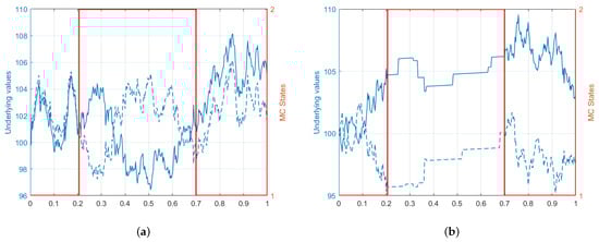
Figure 1.
(a) Sample paths in the case of positively/negatively correlated diffusive component. The red stair-graph represents the realized states of the underlying Markov chain. (b) Sample paths for a mixed model only with a diffusive component (regime 1) or jump component (regime 2).
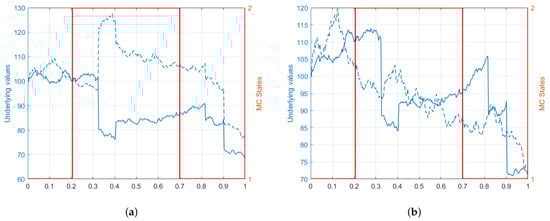
Figure 2.
(a) Sample paths in the case of highly correlated (regime 1) and highly anti-correlated (regime 2) common jumps. (b) Sample paths in the case when the common jumps only impact one asset.
In the second set of Monte Carlo experiments, we show the joint behavior of the couple for some choice of the parameters. In particular, in Figure 3a, the scatter plot is reported in the case of diffusive components only, which is highly positively correlated in regime 1 and anti-correlated in regime 2; in Figure 3b, the dynamic is characterized by a negatively correlated diffusive component in regime 1 and only a systematic compound Poisson process in regime 2 with positively correlated Gaussian co-jumps. Similarly, in Figure 4a,b, we simulated the asymmetric Laplace jumps model: in the left figure, both regimes are characterized by independent diffusion processes, idiosyncratic jumps with positive and negative location parameters only in regime 1, and no systematic jumps. In the figure, on the right, the diffusive component is again independent, but only common jumps are considered, positively correlated in regime 1 and negatively correlated in regime 2. The location parameters have the same magnitude but an inverted sign in the two regimes. The asymmetry is due to the different co-jump intensity across the regimes.
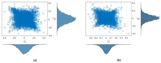
Figure 3.
(a) Scatter plot for the joint states of regime-switching diffusion at time . In this experiment, the processes are positively correlated in regime 1 and negatively correlated in regime 2. (b) Scatter plot in the case of a negatively correlated diffusive component in regime 1 and a positively correlated co-jump distribution in regime 2.
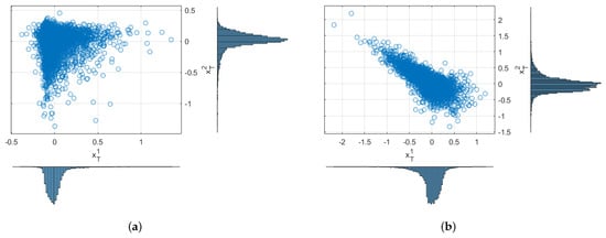
Figure 4.
(a) Scatter plot for the joint states of a regime-switching diffusion at time . In this experiment, the processes are positively correlated in regime 1 and negatively correlated in regime 2; (b) Scatter plot in the case of negatively correlated diffusive component in regime 1 and positively correlated co-jump distribution in regime 2.
3. Spread Option Pricing: The Caldana–Fusai Approximation
By following the classical risk-neutral pricing method, the derivative price at time , , is given by the discounted expectation of the payoff with respect to an equivalent martingale measure. In general, the spread option does not have an explicit solution even in the Black and Scholes framework (except for the case , i.e., the exchange or Margrabe option) and a few methods were developed, such as the popular approximation given by the formula of Kirk (1995), which is the current market standard. In [4], the authors propose a lower bound for to improve the well-known Kirk’s approximation: this lower bound is obtained by considering the following payoff
where is the indicator function and are given parameters. The risk-neutral expectation of the pay-off (7) gives the approximated price: it is made up by three terms that are explicitly computed in the classical bivariate log-normal process framework for . By applying a Monte Carlo simulation procedure to approximate the true spread option price, the numerical results presented show that their formula is more accurate than Kirk’s approximation, even with a canonical choice for the parameters a and k.
In [5], the same technique was extended using a Fourier-based approach. Thus, it can be applied to a more extensive set of market dynamical models, essentially whenever the bivariate Fourier transform, or characteristic function for is analytically available (and the standard integrability conditions are satisfied). The approximate price is therefore given by
which can be represented in terms of the inverse Fourier transform: the following proposition is proved in [5].
Proposition 2.
Let be the characteristic function of . By fixing a dumping parameter , the approximate price of a spread option is given by
where
The approximation can be optimized with respect to the parameters a and k: as suggested in [4], a very efficient choice is given by and , where is the forward price of the second asset with delivery T. The optimized approximation is obtained by maximizing the lower bound for the price (see [5]).
The approximation proved to be very tight, providing estimates comparable to the benchmark Monte Carlo prices. Furthermore, it is computationally appealing in the class of Fourier-based techniques: the approximated option price is obtained through a univariate Fourier inversion, while similar approaches such as that proposed in [6] require a bivariate Fourier inversion. An upper bound is also available (see Section in [5]).
Furthermore, from Proposition 2, assuming that it is possible to interchange integration and differentiation, the Greeks are immediately approximated as
being the variable defining the Greek.
Exchange Option Pricing
The Caldana–Fusai approach gives the exact price for the Exchange Option, i.e., when . In fact, in such a case, by taking and we immediately have that . In a Gaussian setting, the price of such an option has a closed form, given by the well-known Margrabe formula. The present approach therefore generalizes the formulas in [10] by allowing for different choices of the jumps law and the possibility of switching between market regimes. Furthermore, the switching behavior of the volatility parameter makes the considered dynamic a stochastic volatility model: the pricing problem in such a framework is generally faced by Monte Carlo techniques or approximation techniques, such as that based on expansion with respect to some model parameters (e.g., [17] or [18]).
4. Numerical Results
In order to assess the performances of the pricing methods, we consider a regime switching dynamic driven by a two-state Markov chain, i.e., . The pricing Formula (9) may be evaluated by using standard integration routines: in particular, we implemented our valuation model in the MatLab© (R2021b) environment, using the build-in integration algorithms.
The evaluation of the characteristic function of the regime-switching jump diffusion requires the following steps:
- (1)
- Calculate (see Proposition 1);
- (2)
- Form the matrix ;
- (3)
- Calculate the matrix exponential .
When , a simpler formula for can be explicitly obtained (see [14]).
We compare the results with Monte Carlo estimates: the sampler from the regime-switching dynamic (3) was obtained by exploiting the process representation in terms of the sojourn times of the underlying Markov chain (see Formula (4)). A variance reduction scheme for the MC estimators and the control variates were also considered. In particular, as suggested in [5], we used the random variable as the control (as can be seen in (7)): this choice implies the estimator
where is an independent sample of the underlying chainsand (as can be seen, e.g., in [2]). We used independent samples.
In our RSJD2 model, in addition to the diffusive part, we may consider different kinds of (univariate and bivariate) jump distributions, whenever their joint characteristic function is available in closed form. Gaussian, asymmetric Laplace as well as other kinds of heavy tails and skewed distribution can be included in our implementation. In all our experiments, we set , , the risk-free rate is and the time to maturity is year. The strikes prices K range from 0 (the exchange or Margrabe option) to the value with step . The Markov chain intensities are and . No dividends were considered. In Table 1, we report the results relative to a diffusive case (no jumps) with negatively correlated Brownians in regime 1, , and positively correlated ones in regime 2, . The other parameters were fixed to , , and . In Table 2, we considered the Gaussian jump diffusion model (Example 1) with independent Brownians () and the same volatilities as before. The jump processes are characterized by the following parameters: , and (only idiosyncratic shocks in regime 1) with and , ; in regime 2, we set , with the same jump amplitudes, and with , and a co-jump correlation equal to . This choice models the case in which the systematic shocks have an only impact during regime 2. Finally, in Table 3, we show the effectiveness of the approximation in the asymmetric Laplace jump diffusion model (Example 2). The set of parameters is the same as the previous example for both regimes 1 and 2, e.g., the same diffusive components, intensities of the three Poisson processes, and the same location and scale parameters but for asymmetric Laplace jump amplitudes.

Table 1.
Numerical results for the regime-switching diffusive model. In parenthesis, the standard deviation of the MC and MC with control variate estimators is given.
Table 2.
Numerical results for the regime-switching Gaussian jump diffusion. In parenthesis, the standard deviation of the MC and MC with control variate estimators is given.
Table 3.
Numerical results for the regime-switching asymmetric Laplace jump diffusion. In parenthesis, the standard deviation of the MC and MC with control variate estimators is given.
In order to assess the quality of the approximation formula, we show the absolute error obtained by varying some model parameters with respect to the benchmark Monte Carlo with control variates. In particular, we varied the correlation coefficients of the diffusive components (Figure 5a,b for the regime-switching jump diffusion Gaussian model) and the correlations of the co-jumps (Figure 6a,b for the regime-switching jump diffusion Gaussian model and Figure 7a,b for the asymmetric Laplace model), with all the other parameters remaining fixed. As before, for the Monte Carlo approximation, we generated independent samples. We may notice that the error is essentially constant with respect to the correlations but it tends to be increasing with regard to the spread level K. The lowest error is obtained for exchange options (), for which the price (9) is exact. Similar results are obtained for other sets of parameters.
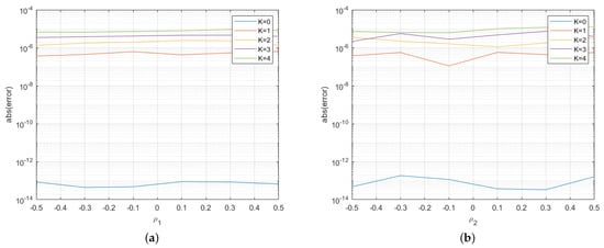
Figure 5.
(a) Approximation error plot for the regime-switching jump diffusion Gaussian model obtained by varying the diffusive correlation in regime 1; and (b) approximation error plot for the regime-switching jump diffusion Gaussian model obtained by varying the diffusive correlation in regime 2.
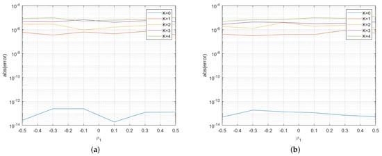
Figure 6.
(a) Approximation error plot for the regime-switching jump diffusion Gaussian model obtained by varying the co-jump correlation in regime 1; and (b) approximation error plot for the regime-switching jump diffusion Gaussian model obtained by varying the co-jump correlation in regime 2.
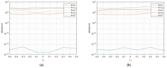
Figure 7.
(a) Approximation error plot for the regime-switching jump diffusion asymmetric Laplace model obtained by varying the co-jump correlation in regime 1; and (b) approximation error plot for the regime-switching jump diffusion asymmetric Laplace model obtained by varying the co-jump correlation in regime 2.
All the pricing algorithms ran on an Intel(R) Core(TM) i7-4700MQ CPU @ 2.40 GHz: the Monte Carlo sampler spent approximately 300 s for the computation of each price, while the Fourier-based method took approximately 0.003 s.
5. Conclusions
We considered the problem of pricing spread and exchange European options using the Caldana–Fusai approximation method in a bivariate regime-switching jump diffusion model. This new class of stochastic models is flexible enough. This allows capturing the joint behavior of the two underlying chains explicitly modeling idiosyncratic and systematic random shocks in a regime-switching environment, which enables characterizing structural changes under market conditions.
The need to have efficient pricing methodologies to evaluate spread options is particularly relevant, as this type of option is widely used in markets as diverse as the energy markets and commodity futures markets, fixed income markets, and foreign exchange and currency markets. Therefore, being able to price the different types of spread options is an important challenge for traders, analysts, and risk managers.
To implement the Fourier-based method proposed in [5] we derived the joint characteristic function of the process and a representation of it based on the sojourn times of the underlying Markov chain. These results also allow us to comprehensively characterize this class of stochastic processes. Furthermore, we derived two Monte Carlo schemes, one for simulating the paths of the two underlying chains, which can be used for pricing path-dependent derivatives, and the second for simulating the underlying values only at maturity. The latter is based on the representation of the random variables in terms of the Markov chain sojourn times, and it was used as a benchmark in our numerical tests. The approximations obtained for the spread option are very accurate with regard to Monte Carlo prices, and they confirm the features of the technique in our regime-switching market model.
New challenges can be outlined in this context, however, such as the extension of the valuation process to American style spread/exchange options, for which the early exercise feature increases the difficulty of the pricing procedures (as can be seen, e.g., in [19,20,21]). On the other hand, since spread options are mainly traded in OTC markets, a relevant issue in their pricing is the inclusion of credit risk in the valuation process. This amount to consider that the derivative is subject to some default event concerning the solvability of one of the counterparties before the transaction settlement. An immediate consequence is that the product’s price needs an adjustment to include the possibility of default in its quotation. These adjustments are generally known as credit valuation adjustment (CVA) and debt valuation adjustment (DVA), depending on which the counterparty suffers the default event. Such events are typically described by employing a random time (i.e., the time of default), using intensity-based models, as can be seen in [22], or structural Merton models, as can be seen in [23]. An application of this last class of models to price spread options in a jump diffusion setting was proposed in [24]. The main difficulties rely on the fact that the default time might not be completely measurable with respect to the information generated by the market prices only and that even under full knowledge of this random time, the derivative’s evaluation will depend on the joint distribution of the random time and price processes. All this requires the definition of suitable computational techniques: for an application to the valuation of plain vanilla options, please see for example [25,26,27] for stochastic volatility model. The efficient pricing of defaultable spread/exchange options and the inclusion of other types of price adjustments, the XVAs, is, therefore, a challenging topic for future research.
Funding
This research received no external funding.
Institutional Review Board Statement
Not applicable.
Informed Consent Statement
Not applicable.
Data Availability Statement
Not applicable.
Acknowledgments
The Author would like to thank G. Fusai for the many valuable suggestions for the software implementation of the model, and the anonymous Referees for the careful reading of the paper. A preliminary version of this work appeared in the Proceedings of the 2nd International Conference on Computational Finance ICCF 2017.
Conflicts of Interest
The authors declare no conflict of interest.
Appendix A
Sketch of the proof of the representation of in terms of the occupation times.
Let us define the occupation times for the m-state Markov chain in : , , being the indicator function of the event A. We immediately have that . Now, given a sample path of the chain , we can define
Since each is the union of non overlapping intervals, the corresponding random variables and are distributed as a Poisson variable and as a Normal variable , respectively. Furthermore, , , for (Here, means that X and Y are independent.) and . By denoting with the k-th jump magnitude relative to regime i and asset j and with , the co-jump components, we have
By defining , and
then admits the following representation:
Appendix B. (Proof of Proposition (6))
From the representation (A4), (A5) we can calculate the characteristic function of the random variable by using the tower property of conditional expectations, . We have
The first expected value is obtained as
The other expectations, since for and , are given by
By recalling the definition of , and defining
we finally have
Actually, the exponent in (A6) is a linear function of the sojourn times , the characteristic function of which are well-known. In fact, it can be proved that
(see, e.g., [20]) from which we have
where , being . Hence the result immediately follows since .
References
- Carmona, R.; Durrleman, V. Pricing and hedging spread options. SIAM Rev. 2003, 45, 627–685. [Google Scholar] [CrossRef] [Green Version]
- Glasserman, P. Monte Carlo Methods in Financial Engineering; Springer: New York, NY, USA, 2004. [Google Scholar]
- Kirk, E. Correlation in the energy market. In Managing Energy Price Risk, 1st ed.; Risk Publication: London, UK, 1995; pp. 71–78. [Google Scholar]
- Bjerksund, P.; Stensland, G. Closed form spread option valuation. Quant. Financ. 2011, 14, 1785–1794. [Google Scholar]
- Caldana, R.; Fusai, G. A general closed-form spread option pricing formula. J. Bank. Financ. 2013, 37, 4893–4906. [Google Scholar] [CrossRef] [Green Version]
- Hurd, T.R.; Zhou, Z. A Fourier Transform Method for Spread Option Pricing. SIAM J. Financ. Math. 2010, 1, 142–157. [Google Scholar] [CrossRef]
- Venkatramana, A.; Alexander, C. Closed form approximations for spread options. Appl. Math. Financ. 2011, 18, 447–472. [Google Scholar] [CrossRef]
- Alfeus, M.; Schlögl, E. On spread option pricing using two-dimensional Fourier transform. Int. J. Theor. Appl. Financ. 2019, 22, 1950023. [Google Scholar] [CrossRef]
- Belle, J.V.; Vanduffel, S.; Yao, J. Closed-form approximations for spread options in Lévy markets. Appl. Stoch. Model. Bus. Ind. 2018, 35, 732–746. [Google Scholar] [CrossRef]
- Cheang, G.H.L.; Chiarella, C. Exchange option under jump-diffusion dynamics. Appl. Math. Financ. 2011, 18, 245–276. [Google Scholar] [CrossRef]
- Petroni, N.C.; Sabino, P. Pricing exchange options with correlated jump diffusion processes. Quant. Financ. 2020, 20, 1811–1823. [Google Scholar] [CrossRef]
- Garces, L.P.D.M.; Cheang, G.H.L. A numerical approach to pricing exchange options under stochastic volatility and jump-diffusion dynamics. Quant. Financ. 2021, 21, 2025–2054. [Google Scholar] [CrossRef]
- Elliott, R.J.; Siu, T.K.; Chan, L.; Lau, J.W. Pricing Options Under a Generalized Markov-Modulated Jump-Diffusion Model. Stoch. Anal. Appl. 2007, 25, 821–843. [Google Scholar] [CrossRef]
- Ramponi, A. On Fourier Transform Methods for Regime-Switching Jump-Diffusions and the pricing of Forward Starting Options. Int. J. Theor. Appl. Financ. 2012, 15, 1250037. [Google Scholar] [CrossRef] [Green Version]
- Kou, S.G. A Jump-Diffusion Model for Option Pricing. Manag. Sci. 2002, 48, 1086–1101. [Google Scholar] [CrossRef] [Green Version]
- Cont, R.; Tankov, P. Financial Modelling with Jump Processes; Chapman & Hall: London, UK, 2004. [Google Scholar]
- Antonelli, F.; Ramponi, A.; Scarlatti, S. Exchange option pricing under stochastic volatility: A correlation expansion. Rev. Deriv. Res. 2010, 13, 45–73. [Google Scholar] [CrossRef] [Green Version]
- Duffie, D.; Pan, J.; Singleton, K. Transform analysis and asset pricing for affine jump-diffusions. Econometrica 2000, 68, 1343–1376. [Google Scholar] [CrossRef] [Green Version]
- Boyarchenko, S.; Levendorskii, S. American Options in Regime-Switching Models. SIAM J. Control. Optim. 2009, 48, 1353–1376. [Google Scholar] [CrossRef]
- Buffington, J.; Elliott, R.J. American options with regime switching. Int. J. Theor. Appl. Financ. 2002, 5, 497–514. [Google Scholar] [CrossRef]
- Company, R.; Egorova, V.N.; Jódar, L. An Efficient Method for Solving Spread Option Pricing Problem: Numerical Analysis and Computing. Abstr. Appl. Anal. 2016, 2016, 1549492. [Google Scholar] [CrossRef] [Green Version]
- Lando, D. On Cox Processes and Credit Risky Securities. Rev. Deriv. Res. 1998, 2, 99–120. [Google Scholar] [CrossRef]
- Klein, P. Pricing Black-Scholes options with correlated credit risk. J. Bank. Financ. 1996, 20, 1211–1229. [Google Scholar] [CrossRef]
- Li, Z.; Wang, X. Valuing spread options with counterparty risk and jump risk. N. Am. J. Econ. Financ. 2020, 54, 101269. [Google Scholar] [CrossRef]
- Antonelli, F.; Ramponi, A.; Scarlatti, S. CVA and vulnerable options pricing by correlation expansions. Ann. Oper. Res. 2019, 299, 401–427. [Google Scholar] [CrossRef] [Green Version]
- Alòs, E.; Antonelli, F.; Ramponi, A.; Scarlatti, S. CVA and vulnerable options in stochastic volatility models. Int. J. Theor. Appl. Financ. 2021, 24, 1–34. [Google Scholar] [CrossRef]
- Alòs, E.; Antonelli, F.; Ramponi, A.; Scarlatti, S. CVA in fractional and rough volatility models. arXiv 2022, arXiv:2204.11554. [Google Scholar]
Publisher’s Note: MDPI stays neutral with regard to jurisdictional claims in published maps and institutional affiliations. |
© 2022 by the author. Licensee MDPI, Basel, Switzerland. This article is an open access article distributed under the terms and conditions of the Creative Commons Attribution (CC BY) license (https://creativecommons.org/licenses/by/4.0/).